


 Abstract
 HTML
HTML Reference
 Related
 PDF
PDF


-
Study on the structure and properties of SHN has been a challenging and attractive subject for researchers [1−5]. Recent years, due to the construction of a new generation of accelerators and the development of the detection technology, the synthesis of elements with Z≤118 have been achieved through the hot fusion reaction with
$ ^{48} {\rm{Ca}}$ as a projectile or cold fusion using the double magic target$ ^{208} {\rm{Pb}}$ or its neighbor$ ^{209} {\rm{Bi}}$ as a target [6−19]. In synthesis, due to the extremely low production cross sections and short lifetimes of the SHN, it is difficult to directly detect and identify the new elements or isotopes. It is well known that α-decay is one of the main decay modes for SHN and it provides an efficient way for the identification of new superheavy elements or isotopes by detecting the α-decay chains from unknown nuclei to known nuclei with the help of the parent-daughter correlation [11, 20, 21]. Moreover, study on α-decay contributes to provide some reliable information on the nuclear structure including ground-state lifetime, released energies, magic numbers, spin-parity, and nuclear interaction [7, 22−27]. Hence, the α-decay plays an indispensable role in theoretical and experimental studies of SHN.α-decay was firstly explained in the 1920s by Gamow [28] and by Gurney and Condon [29] as a fundamental quantum tunneling effect, which is considered to be the first successful quantum description on nuclear phenomenon. From then on, based on this physical picture numerous phenomenological and microscopic models, such as effective liquid drop model [30−33], generalized liquid drop model [34, 35], cluster model [36−40], density-dependent M3Y effective interaction [41, 42] and unified fission model [43−45], have been developed to pursue a quantitative description of α-decay half-lives. In addition, a series of semi-empirical formulas, such as the Royer formula [46], universal decay law [47−51] and universal formula [52−54], have been proposed to calculate the α-decay half-lives. It has been found that these models and semi-empirical formulas can reproduce the experimental α-decay half-lives more or less satisfactorily [30−54].
As the view of the preformation model,
$S _{\alpha } $ is an important physical quantity for α-decay half-life. However, it is difficult to obtain the accurate$S _{\alpha } $ values of various nuclei. So, when ones estimate the α-decay half-lives, the empirical$S _{\alpha } $ values have to be used [53, 55−58]. Moreover, these$S _{\alpha } $ values are strongly dependent on the models [59]. As a result, the order of magnitude of the calculated half-life is different when ones employe the$S _{\alpha } $ values extracted from different models. So it is very important and necessary to use a model that can calculate the$S _{\alpha } $ values reasonably to estimate the α-decay half-lives. Among the numerous α-decay models, the one-parameter model proposed by Tavares et al. is such a model that can estimate α-decay half-lives accurately because the$S _{\alpha } $ values can be extracted by a WKB-integral approximation [60]. Furthermore, the proton and cluster radioactivity were described successfully by this model [61−63]. Recent years, some new SHN have been synthesized and lots of experimental data on α-decay have been measured. Therefore, these experimental data becomes a ground to test the one-parameter model. So it is necessary to extend this model to study the α-decay half-lives of SHN. This constitutes the first motivation of this article. Moreover, the synthesis of Z = 119 and 120 elements are the next aim for the nuclear scientists [64−66], so the second motivation of present study is to predict the α-decay half-lives of Z = 119 and 120 isotopes or their neighbors within this model. We hope these predictions are helpful for future experiments.This article is organized as follows. In Sec. II the theoretical framework is introduced. Results and discussions are presented in Sec. III. In the last section, some conclusions are given.
-
Generally, the half-life of α-decay is calculated by the following expression:
$T _{1/2} = \lambda ^{-1}\ln 2 $ , where$T _{1/2} $ is the half-life and λ is the decay constant. In the framework of the one-parameter model [60−63], λ is calculated by$ \lambda = \lambda _{0}S_{\alpha }P_{se},\;\;\;\;S_{\alpha } = e^{-G_{ov}},\;\;\;\;P_{se} = e^{-G_{se}}, $

(1) where
$ \lambda _{0} $ is the assault frequency on the barrier,$ G_{ov} $ represents the Gamow factor calculated in the overlapping barrier region where the α-particle drives away from the parent nucleus until it reaches the contact configuration, while$ G_{se} $ denotes the Gamow factor determined in the external, separation region which spans from the aforementioned contact configuration to the separation point and$ P_{se} $ is the corresponding penetration probability of the α-particle.Usually, the quantity of
$ \lambda _{0} $ is estimated as$ \lambda _{0} = \frac{\upsilon }{2a} = \frac{2^{1/2}}{2a}\left(\frac{Q_{\alpha }}{\mu _{0}}\right)^{1/2}, $

(2) where υ is the relative velocity of the fragments and
$ a = R_{p}-R_{a} $ is the difference between the radius of the parent nucleus and the α-particle radius.$ \mu _{0} $ is the final reduced mass of the system. In this work, it is defined as$ \mu _{0} = \dfrac{A_{d}A_{e}}{A_{d}+A_{e}}m_{p} $ . Here,$ A_{d} $ and$ A_{e} $ stand for the mass number of the daughter nucleus and the emitted particle, respectively.$ m_{p} $ denotes the nucleon mass.In Eq. (1),
$ G_{ov} $ and$ G_{se} $ are both calculated by the WKB-integral approximation and their expressions can be written as$ G_{ov} = \frac{2}{\hbar }\int_{a}^{c}\sqrt{2\mu _{ov}(r)[V_{ov}(r)-Q_{\alpha }] }dr, $

(3) $ G_{se} = \frac{2}{\hbar }\int_{c}^{b}\sqrt{2\mu _{se}(r)[V_{se}(r)-Q_{\alpha }] }dr, $

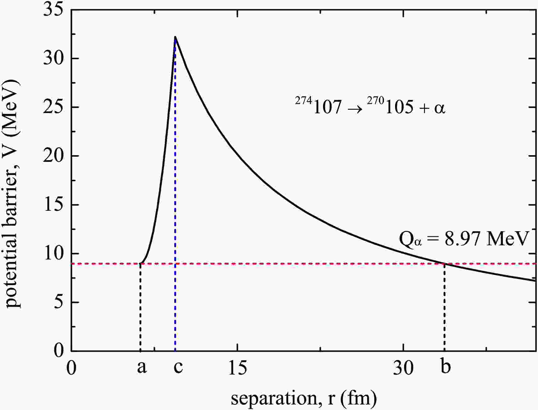
(4) where ħ is the reduced Planck constant, r is the center-of-mass distance between the emitted α-particle and the daughter nucleus,
$ c = R_{d}+R_{\alpha } $ is the separation of fragments in the contact configuration and b denotes the separation point where the total potential energy satisfies the condition$ V(b) = Q_{\alpha } $ . Here,$R _{\alpha} $ is the charge radius of α-particle, whose value is 1.62 fm in this work.$R _{p} $ and$R _{d} $ are the radius of the parent and daughter nucleus, whose values are evaluated by the droplet model. The corresponding expressions are$ R_{i} = \frac{Z_{i}}{A_{i}}R_{p'i}+\left(1-\frac{Z_{i}}{A_{i}}\right)R_{n'i},\;\;\;\;i = p,d, $

(5) where
$R _{p'i} $ and$R _{n'i} $ are given by$ R_{ji} = r_{ji}\left[ 1+\frac{5}{2}\left( \frac{w}{r_{ji}}\right) ^{2}\right] ,\;\;\;\;j = p',n';\;\;i = p,d, $

(6) where w = 1 fm denotes the diffuseness of the nuclear surface.
$r _{ji} $ represent the equivalent sharp radius of a proton (j =$ p' $ ) or neutron (j =$ n' $ ) density distribution of the parent nucleus (i = p) or daughter nucleus (i = d), respectively. According to the finite-range droplet model theory of nuclei proposed by Möller et al., the equivalent sharp radius can be extracted from the following expressions$ r_{p'i} = r_{0}(1+\overline{\epsilon _{i}})\left[ 1-\frac{2}{3}\left(1-\frac{Z_{i}}{ A_{i}}\right)\left(1-\frac{2Z_{i}}{A_{i}}-\overline{\delta _{i}}\right)\right] A_{i}^{1/3}, $

(7) $ r_{n'i} = r_{0}(1+\overline{\epsilon _{i}})\left[ 1+\frac{2}{3}\frac{Z_{i}}{ A_{i}}\left(1-\frac{2Z_{i}}{A_{i}}-\overline{\delta _{i}}\right)\right] A_{i}^{1/3}, $

(8) where
$r _{0} $ = 1.16 fm, i = p (parent) or d (daughter), and$ \overline{\epsilon _{i}} $ and$ \overline{\delta _{i}} $ can be given by$ \overline{\epsilon _{i}} = \frac{1}{4\mathrm{e}^{0.831A_{i}^{1/3}}}-\frac{0.191}{ A_{i}^{1/3}}+\frac{0.0031Z_{i}^{2}}{A_{i}^{4/3}}, $

(9) $ \overline{\delta _{i}} = \left(1-\frac{2Z_{i}}{A_{i}}+0.004781\frac{Z_{i}}{ A_{i}^{2/3}}\right)\Bigg/\left(1+\frac{2.52114}{A_{i}^{1/3}}\right). $

(10) In the overlapping barrier region (a≤r≤c, see Fig. 1), the reduced mass of the disintegration system
$ \mu _{ov}(r) $ and the potential barrier$ V_{ov}(r) $ appear in Eq. (3) can be expressed as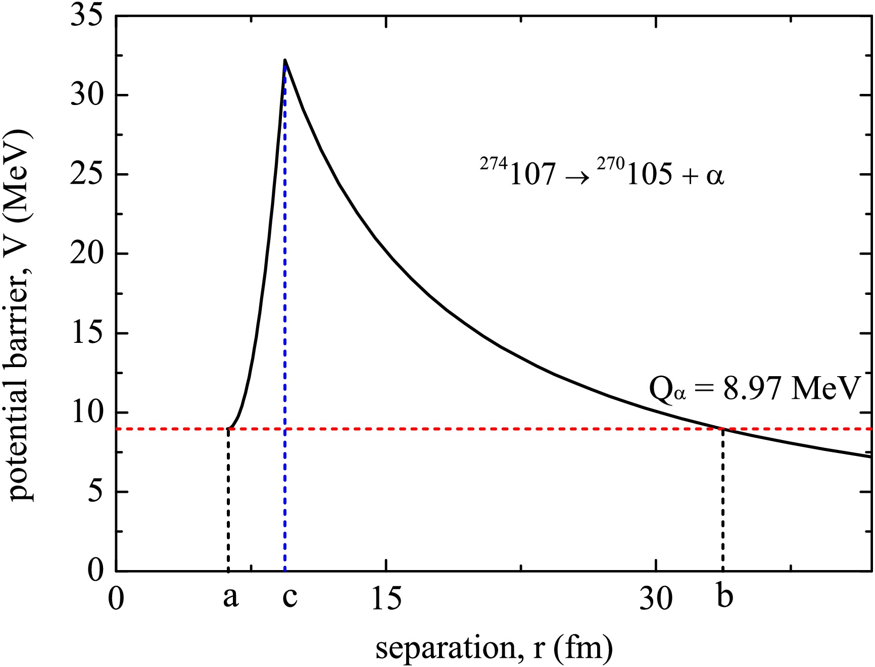
Figure 1. (Color online) The shape of the one-dimensional potential barrier for α-decay of
$ ^{274} {\rm{107}}$ . The barrier from a to c is the overlapping region and that from c to b is the separation region.$ \mu _{ov}(r) = \mu _{0}\left(\frac{r-a}{c-a}\right)^{\chi},\;\;\;\;\chi\geqslant 0, $

(11) $ V_{ov}(r) = Q_{\alpha }+(V_{c}-Q_{\alpha })\left(\frac{r-a}{c-a}\right)^{q},\;\;\;\;q\geqslant 1, $

(12) with
$ V_{c} = \frac{2Z_{d}e^{2}}{c}+\frac{l(l+1)\hbar ^{2}}{2\mu _{0}c^{2}}, $

(13) in which
$e ^{2} $ = 1.4399652 MeV fm. l and$Z _{{d}} $ represent the angular momentum carried by the α-particle and the charge number of the daughter nucleus, respectively. The mass power parameter χ in Eq. (11) and potential energy power parameter q in Eq. (12) are employed to characterize the variations of$ \mu _{ov}(r) $ and$ V_{ov}(r) $ in the overlapping region. According to Eqs. (3) and (11-13), the Gamow factor$ {G}_{{ov}} $ is analytically given by${ G_{ov} = 0.4374702(c-a)g\left\{ \mu _{0}\left[\dfrac{2Z_{d}e^{2}}{c}+\dfrac{ 20.9008l(l+1)}{\mu _{0}c^{2}}-Q_{\alpha }\right]\right\} ^{1/2}, }$

(14) where
$ g = \left(1+\frac{\chi+q}{2}\right)^{-1},\;\;\;\;0<g\leqslant 2/3, $

(15) is the unique adjustable parameter of the model, the value of which is determined from a set of measured half-life values. According to Eqs. (11), (12) and (15), it is easy to see that the parameter g is correlated to the reduced mass and interaction potential in the overlapping region.
In the separation region (c≤r≤b, see Fig. 1), the corresponding reduced mass of the disintegration system
$ \mu _{se}(r) $ becomes a constant. Meanwhile, the potential barrier$ V_{se}(r) $ comprises superposition of the Coulomb and centrifugal potential barriers. As a result, the$ \mu _{se}(r) $ and$ V_{se}(r) $ can be given by$ \mu _{se}(r) = \mu _{0}, $

(16) $ V_{se}(r) = \frac{2Z_{d}e^{2}}{r}+\frac{l(l+1)\hbar ^{2}}{2\mu _{0}r^{2}}. $

(17) Combing Eqs. (4), (16) and (17), the Gamow factor
$ {\rm{G}}_{se} $ is given by a simple analytic form as$ G_{se} = 1.25988372Z_{d}\left(\frac{\mu _{0}}{Q_{\alpha }} \right)^{1/2}[F(x,y)+H(x,y)-f(x,y)], $

(18) with
$ F(x,y) = \frac{x^{1/2}}{2y}\times \ln \frac{[x(x+2y-1)]^{1/2}+x+y}{\dfrac{x}{y} \left[1+\left(1+\dfrac{x}{y^{2}}\right)^{1/2}\right]^{-1}+y}, $

(19) $ H(x,y) = \arccos \left\{\frac{1}{2}\left[1-\dfrac{1-\dfrac{1}{y}}{\left(1+\dfrac{x}{y^{2}}\right)^{1/2} }\right]\right\}^{1/2}, $

(20) $ f(x,y) = \left[\frac{1}{2y}\left(1+\frac{x}{2y}-\frac{1}{2y}\right)\right]^{1/2}, $

(21) where
$ x = \frac{20.9008l(l+1)}{\mu _{0}c^{2}Q_{\alpha }},\;\;\;\;y = \frac{Z_{d}e^{2}}{ cQ_{\alpha }}. $

(22) Finally, the half-life of α-decay is calculated by
$ T_{1/2} = 1.0\times 10^{-22}a\left(\frac{\mu _{0}}{Q_{\alpha }}\right)^{1/2}\mathrm{e} ^{G_{ov}+G_{se}}. $

(23) -
To proceed with a systematic analysis of the α-decay half-lives of SHN with Z≥104, firstly we need to determine the g-value of Eq. (14), which has a certain influence on the strength of
$S _{\alpha } $ as well as the half-lives. Since the standard deviation (σ) represents the difference between the experimental half-lives and the calculated ones, so in this work we follow the practice of Ref. [60] to find the optimal g-value by the minimizing σ within the following formula$ \sigma = \left[ \frac{1}{n}\sum\limits_{i = 1}^{n}(\log _{10}T_{1/2}^{\text{expt.}i}-\log _{10}T_{1/2}^{\text{cal.}i})^{2}\right] ^{1/2}, $

(24) where
$ \log _{10}T_{1/2}^{\text{expt.}} $ and$ \log _{10}T_{1/2}^{\text{cal.}} $ are the decimal logarithms of the experimental and calculated half-lives, respectively. n is the number of α-decay events of SHN. By inputting the experimental$ Q_{\alpha } $ values and half-lives taken from Refs. [6−20, 68−71], the process for determining the optimal g-value is plotted in Fig. 2. From Fig. 2 it can be seen that the parameter g is determined to be 0.2038 when the minimum σ ($ \sigma _{\min } $ ) equals to 0.5127. Then the half-lives of the 81 α-emitters are calculated within the one-parameter model by inputting the obtained optimal g-value. The detailed calculated results are listed in Table 1. In Table 1, column 1 represents the parent nuclei. Column 2 denotes the experimental$ Q_{\alpha } $ values. The$S _{\alpha } $ values extracted by Eqs. (1), (14) and (15) are shown in column 3. Columns 4 and 5 are the decimal logarithms of the experimental half-lives and those of the calculated half-lives, respectively. Note that for α-decay of these SHN, the l values are selected as 0 because their spin-parities are not available. Therefore, the centrifugal potential contribution to the half-life is not taken into account. From Table 1, one can see that the$S _{\alpha } $ values are located between 6.12$ \times $ 10−2 and 7.15$ \times $ 10−2, whose order of magnitude is consistent with those of the generalized liquid drop model [35, 72] and the study reported by Ismail et al. [73]. Next, to show the global deviation quantitatively, besides the above mentioned σ values, the average deviation$ \overline{\sigma } $ is calculated by the following expression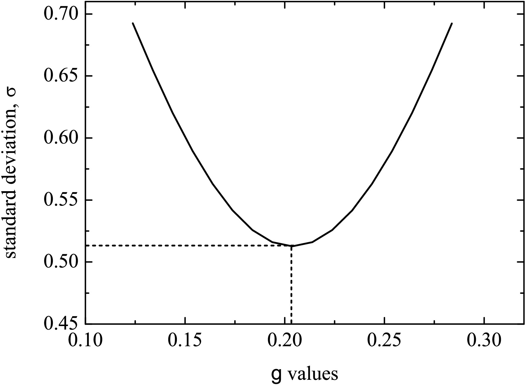
Figure 2. The standard deviation σ as a function of the g values.
Nuclei $ Q_{\alpha } \;{\rm{(MeV)}} $ 

$ S_{\alpha }(10^{-2}) $ 

$ \log _{10}T_{1/2}^{\text{expt.}} \;{\rm{(s)}} $ 

$ {\log }_{10}T_{1/2}^{\text{cal.}} \;{\rm{(s)}} $ 

$ \log _{10}HF $ 

$ ^{255} {\rm{104}}$ 

9.05 [67] 6.63 0.65 [67] 0.39 0.26 $ ^{256} {\rm{104}}$ 

8.93 [68] 6.59 0.32 [71] 0.75 −0.43 $ ^{258} {\rm{104}}$ 

9.19 [68] 6.72 −0.97 [71] −0.08 −0.90 $ ^{259} {\rm{104}}$ 

9.13 [67] 6.70 0.41 [67] 0.09 0.33 $ ^{261} {\rm{104}}$ 

8.65 [68] 6.53 0.91 [71] 1.55 −0.64 $ ^{263} {\rm{104}}$ 

8.25 [67] 6.40 3.30 [67] 2.87 0.43 $ ^{256} {\rm{105}}$ 

9.34 [68] 6.63 0.45 [71] −0.13 0.58 $ ^{257} {\rm{105}}$ 

9.21 [67] 6.59 0.39 [67] 0.25 0.14 $ ^{258} {\rm{105}}$ 

9.50 [67] 6.72 0.75 [67] −0.61 1.36 $ ^{259} {\rm{105}}$ 

9.62 [68] 6.78 −0.29 [71] −0.97 0.67 $ ^{270} {\rm{105}}$ 

8.02 [6] 6.27 3.56 [6] 4.00 −0.44 $ ^{259} {\rm{106}}$ 

9.80 [68] 6.73 −0.51 [71] −1.12 0.62 $ ^{260} {\rm{106}}$ 

9.90 [68] 6.78 −1.91 [71] −1.40 −0.51 $ ^{261} {\rm{106}}$ 

9.71 [68] 6.72 −0.73 [71] −0.91 0.18 $ ^{263} {\rm{106}}$ 

9.40 [68] 6.61 0.03 [71] −0.05 0.08 $ ^{267} {\rm{106}}$ 

8.32 [7] 6.25 2.80 [7] 3.34 −0.54 $ ^{269} {\rm{106}}$ 

8.70 [68] 6.41 2.68 [71] 2.03 0.65 $ ^{271} {\rm{106}}$ 

8.66 [8] 6.41 2.21 [8] 2.14 0.08 $ ^{260} {\rm{107}}$ 

10.4 [67] 6.86 −1.46 [67] −2.35 0.90 $ ^{261} {\rm{107}}$ 

10.5 [67] 6.92 −1.93 [67] −2.61 0.69 $ ^{265} {\rm{107}}$ 

9.38 [9] 6.51 −0.03 [9] 0.34 −0.37 $ ^{266} {\rm{107}}$ 

9.43 [10] 6.54 0.40 [10] 0.18 0.22 $ ^{267} {\rm{107}}$ 

8.96 [10] 6.37 1.34 [10] 1.58 −0.24 $ ^{270} {\rm{107}}$ 

9.06 [67] 6.44 1.78 [67] 1.24 0.54 $ ^{272} {\rm{107}}$ 

9.14 [11] 6.49 0.91 [11] 0.95 −0.04 $ ^{274} {\rm{107}}$ 

8.97 [6] 6.44 1.48 [6] 1.46 0.01 $ ^{264} {\rm{108}}$ 

10.59 [67] 6.86 −2.80 [67] −2.55 −0.24 $ ^{265} {\rm{108}}$ 

10.47 [68] 6.82 −2.71 [71] −2.27 −0.44 $ ^{266} {\rm{108}}$ 

10.35 [67] 6.78 −2.64 [67] −1.97 −0.67 $ ^{268} {\rm{108}}$ 

9.62 [68] 6.52 0.15 [71] −0.05 0.20 $ ^{269} {\rm{108}}$ 

9.32 [12] 6.41 1.18 [12] 0.83 0.36 $ ^{270} {\rm{108}}$ 

9.15 [20] 6.36 0.88 [20] 1.33 −0.45 $ ^{273} {\rm{108}}$ 

9.73 [68] 6.61 −0.04 [71] −0.43 0.39 $ ^{275} {\rm{108}}$ 

9.44 [68] 6.52 −0.54 [71] 0.38 −0.92 $ ^{270} {\rm{109}}$ 

10.18 [68] 6.64 −2.20 [71] −1.26 −0.94 $ ^{274} {\rm{109}}$ 

10.04 [13] 6.63 −0.35 [13] −0.94 0.59 $ ^{275} {\rm{109}}$ 

10.48 [14] 6.82 −2.01 [14] −2.11 0.10 $ ^{276} {\rm{109}}$ 

9.81 [67] 6.56 −0.14 [67] −0.35 0.21 $ ^{278} {\rm{109}}$ 

9.59 [6] 6.49 0.56 [6] 0.25 0.30 $ ^{267} {\rm{110}}$ 

11.78 [68] 7.15 −5.00 [71] −4.67 −0.33 $ ^{269} {\rm{110}}$ 

11.51 [67] 7.06 −3.75 [67] −4.12 0.37 $ ^{270} {\rm{110}}$ 

11.12 [68] 6.90 −3.69 [71] −3.25 −0.44 $ ^{271} {\rm{110}}$ 

10.87 [67] 6.81 −2.79 [67] −2.68 −0.10 $ ^{273} {\rm{110}}$ 

11.37 [67] 7.04 −3.77 [67] −3.87 0.10 $ ^{275} {\rm{110}}$ 

11.37 [70] 7.07 −3.37 [70] −3.90 0.53 $ ^{277} {\rm{110}}$ 

10.83 [67] 6.86 −2.39 [67] −2.67 0.29 $ ^{279} {\rm{110}}$ 

9.84 [8] 6.49 0.30 [8] −0.13 0.43 $ ^{281} {\rm{110}}$ 

8.86 [15] 6.14 2.35 [15] 2.86 −0.51 $ ^{272} {\rm{111}}$ 

11.20 [67] 6.83 −2.42 [67] −3.15 0.73 $ ^{278} {\rm{111}}$ 

10.85 [67] 6.76 −2.38 [67] −2.42 0.04 $ ^{279} {\rm{111}}$ 

10.52 [67] 6.64 −0.77 [67] −1.61 0.84 $ ^{280} {\rm{111}}$ 

9.89 [11] 6.40 0.55 [11] 0.06 0.48 $ ^{281} {\rm{111}}$ 

9.41 [16] 6.24 2.23 [16] 1.45 0.78 $ ^{282} {\rm{111}}$ 

9.08 [6] 6.13 2.27 [6] 2.47 −0.20 $ ^{277} {\rm{112}}$ 

11.62 [67] 6.94 −3.16 [67] −3.86 0.70 $ ^{281} {\rm{112}}$ 

10.46 [67] 6.52 −0.89 [67] −1.15 0.27 $ ^{283} {\rm{112}}$ 

9.67 [17] 6.24 0.58 [17] 1.01 −0.43 $ ^{284} {\rm{112}}$ 

9.30 [18] 6.12 0.99 [18] 2.12 −1.13 $ ^{285} {\rm{112}}$ 

9.32 [68] 6.13 1.51 [71] 2.04 −0.54 $ ^{278} {\rm{113}}$ 

11.85 [67] 6.93 −3.62 [67] −4.07 0.45 $ ^{282} {\rm{113}}$ 

10.78 [67] 6.54 −1.15 [67] −1.65 0.50 $ ^{283} {\rm{113}}$ 

10.26 [14] 6.35 −0.99 [14] −0.31 −0.68 $ ^{284} {\rm{113}}$ 

10.11 [11] 6.30 −0.03 [11] 0.08 −0.10 $ ^{285} {\rm{113}}$ 

9.84 [11] 6.22 0.51 [11] 0.84 −0.33 $ ^{286} {\rm{113}}$ 

9.79 [67] 6.21 1.30 [67] 0.97 0.33 $ ^{285} {\rm{114}}$ 

10.54 [19] 6.36 −0.33 [19] −0.75 0.43 $ ^{286} {\rm{114}}$ 

10.37 [68] 6.31 −0.46 [71] −0.32 −0.14 $ ^{287} {\rm{114}}$ 

10.16 [68] 6.24 −0.28 [71] 0.24 −0.53 $ ^{288} {\rm{114}}$ 

10.07 [68] 6.22 −0.12 [71] 0.48 −0.60 $ ^{289} {\rm{114}}$ 

9.97 [68] 6.19 0.38 [71] 0.75 −0.37 $ ^{287} {\rm{115}}$ 

10.74 [68] 6.35 −0.92 [71] −0.97 0.05 $ ^{288} {\rm{115}}$ 

10.63 [68] 6.32 −0.72 [71] −0.70 −0.02 $ ^{289} {\rm{115}}$ 

10.49 [11] 6.28 −0.70 [11] −0.34 −0.36 $ ^{290} {\rm{115}}$ 

10.45 [6] 6.27 0.11 [6] −0.25 0.37 $ ^{290} {\rm{116}}$ 

10.99 [68] 6.36 −2.10 [71] −1.32 −0.77 $ ^{291} {\rm{116}}$ 

10.89 [68] 6.34 −1.55 [71] −1.08 −0.47 $ ^{292} {\rm{116}}$ 

10.77 [68] 6.30 −1.62 [71] −0.80 −0.82 $ ^{293} {\rm{116}}$ 

10.68 [68] 6.28 −1.10 [71] −0.57 −0.52 $ ^{293} {\rm{117}}$ 

11.18 [69] 6.36 −1.84 [69] −1.51 −0.32 $ ^{294} {\rm{117}}$ 

11.20 [6] 6.37 −1.29 [6] −1.58 0.29 $ ^{294} {\rm{118}}$ 

11.81 [68] 6.49 −2.85 [71] −2.70 −0.15 Table 1. The experimental and calculated α-decay half-lives of SHN with Z
$ \geqslant {\rm{104}}$ .$ \overline{\sigma} = \frac{1}{n}\sum\limits_{i = 1}^{n} \left|\log _{10}T_{1/2}^{\text{expt.}i}-\log _{10}T_{1/2}^{\text{cal.}i}\right|. $

(25) Within Eq. (25), the obtained
$ \overline{\sigma } $ value of 81 SHN is 0.4377. It suggests that the experimental α-decay half-lives are reproduced well by this model.To further analyze the deviation of the experimental half-lives from the calculated ones, the logarithm hindrance factor
$ \log _{10}HF $ is calculated by$ \log_{10}HF = \log _{10}(T_{1/2}^{\text{expt.}}/T_{1/2}^{\text{cal.}}). $

(26) The
$ \log _{10}HF $ values within Eq. (26) are listed in the final column of Table 1 and the$ \log _{10}HF $ values versus the neutron numbers N of parent nuclei are plotted in Fig. 3. Usually, it is believed that if the$ \log_{10}HF $ value is within a factor of 1.0, the calculated half-lives will be in agreement with the experimental data [5, 49, 50]. From the last column of Table 1 and Fig. 3, an agreement between the calculated half-lives and the experimental data is found except for the cases of$ ^{258}105 $ and$ ^{284}112 $ . The agreement implies the assumed$S _{\alpha } $ expression has a certain of rationality. For some models, the inner potential barrier correlated to$S _{\alpha } $ is neglected. To make up for this deficiency, the empirical or constant$S _{\alpha } $ is usually used [58, 74]. As a result, the accuracies and predicted powers of these models are not so satisfactory. But for the one-parameter model, the potential barrier is composed of the inner barrier in the overlapping region and the external barrier in the separation region. The penetrability through the inner part of the potential is considered to represent$S _{\alpha } $ . Furthermore, the correlation between$S _{\alpha } $ and$ Q_{\alpha } $ is taken into account, which can be seen from Eqs. (1) and (14). So, the$S _{\alpha } $ values can be extracted reasonably. Besides, relevant studies suggested that the charge radius has important influence on the α-decay half-life [39, 75, 76]. In the one-parameter model, the accurate radius expressions following the droplet model (Eqs. (5-10)) are included. Based on the two above mentioned reasons, most experimental α-decay half-lives are reproduced well. However, it is necessary to point out that there exist a set of expressions for the charge radius [77−80] except for the radius formulas of droplet model. When other types of radius formulas are used to calculate the α-decay half-life within the one-parameter model, the calculated accuracy will be changed. But if ones want to improve the model accuracy, the parameters of the charge radius formulas need to be refitted using the experimental data of α-decay.
Figure 3. The
$ \log _{10}HF $ values versus the neutron numbers N of parent nuclei for 81 SHN using the one-parameter model.Encouraged by the agreement between the calculated half-lives and the experimental data, we attempted to predict the α-decay half-lives of Z = 118-120 isotopes within the one-parameter model. It is well known that
$ Q_{\alpha } $ values play a crucial role in determining the half-lives. Recent years, various models on the nuclear masses have been developed to obtain the$ Q_{\alpha } $ values. In present work, we select the RCHB [81], DZ19 [82], IMWS [83] and ML [84] mass tables to get the$ Q_{\alpha } $ values through the following relationship$ Q_{\alpha } = M-M_{d}-M_{\alpha }, $

(27) where M,
$ M_{d} $ and$ M_{\alpha } $ represent the mass excesses of the parent nucleus, daughter nucleus and emitted α-particle, respectively.Then, the α-decay half-lives of Z = 118-120 isotopes are calculated by inputting the
$ Q_{\alpha } $ values extracted from the above mentioned four kinds of nuclear mass tables. The$ Q_{\alpha } $ values, corresponding$ S_{\alpha } $ and half-lives of Z = 118-120 isotopes are listed in Table 2. From Table 2, one can see that (i) for a given nucleus the$ Q_{\alpha } $ values extracted from the four types of nuclear mass tables are different. This indicates that$ Q_{\alpha } $ are dependent strongly on nuclear mass models; (ii)$ S_{\alpha } $ is slightly dependent on the$ Q_{\alpha } $ values. Specifically, the larger the$ Q_{\alpha } $ , the larger the$S _{\alpha } $ value, and vice versa; (iii) the half-lives are sensitive to the$ Q_{\alpha } $ values. For example, the$ Q_{\alpha } $ value of$ ^{289} $ 118 given by the RCHB theory is lower 2.82 MeV than that by the DZ19 model, but the corresponding half-life difference is as high as about 7 orders of magnitude. Hence, it is necessary to continue developing a more accurate mass model by taking into account more physical ingredients.Nuclei $Q _{\alpha }^{\mathrm{RCHB}} $ 

(MeV)$Q _{\alpha }^{\mathrm{DZ19}} $ 

(MeV)$Q _{\alpha }^{\mathrm{IMWS}} $ 

(MeV)$Q _{\alpha }^{\mathrm{ML}} $ 

(MeV)$S _{\alpha }^{\mathrm{RCHB}} $ 

($ 10 ^{-2} $ )

$S _{\alpha }^{\mathrm{DZ19}} $ 

($ 10 ^{-2} $ )

$S _{\alpha }^{\mathrm{IMWS}} $ 

($ 10 ^{-2} $ )

$S _{\alpha }^{\mathrm{ML}} $ 

($ 10 ^{-2} $ )

$ {\rm{log}} _{10} $ 

$T _{1/2}^{\mathrm{RCHB}} $ 

(s)$ {\rm{log}}_{10} $ 

$T _{1/2}^{\mathrm{DZ19}} $ 

(s)$ {\rm{log}}_{10} $ 

$T _{1/2}^{\mathrm{IMWS}} $ 

(s)$ {\rm{log}}_{10} $ 

$T _{1/2}^{\mathrm{ML}} $ 

(s)$ ^{289} {\rm{118}}$ 

9.77 12.59 12.09 12.52 5.72 6.75 6.55 6.72 2.76 −4.31 −3.25 −4.17 $ ^{290} {\rm{118}}$ 

9.50 12.38 12.18 12.46 5.65 6.67 6.60 6.71 3.60 −3.88 −3.47 −4.05 $ ^{291} {\rm{118}}$ 

10.27 12.16 12.05 12.35 5.91 6.60 6.55 6.67 1.26 −3.43 −3.19 −3.84 $ ^{292} {\rm{118}}$ 

10.97 11.95 12.07 12.10 6.16 6.53 6.57 6.59 −0.64 −2.99 −3.24 −3.32 $ ^{293} {\rm{118}}$ 

10.94 11.75 11.92 12.17 6.16 6.46 6.53 6.62 −0.58 −2.54 −2.94 −3.48 $ ^{294} {\rm{118}}$ 

10.92 11.56 11.89 12.06 6.16 6.40 6.52 6.59 −0.54 −2.12 −2.87 −3.25 $ ^{295} {\rm{118}}$ 

10.88 11.36 11.78 11.83 6.16 6.33 6.49 6.51 −0.46 −1.67 −2.65 −2.77 $ ^{296} {\rm{118}}$ 

10.78 11.18 11.89 11.61 6.13 6.28 6.55 6.44 −0.21 −1.25 −2.91 −2.27 $ ^{297} {\rm{118}}$ 

10.65 11.00 11.83 12.03 6.09 6.22 6.53 6.61 0.12 −0.81 −2.80 −3.24 $ ^{298} {\rm{118}}$ 

10.62 10.84 11.86 12.04 6.09 6.17 6.55 6.63 0.19 −0.40 −2.87 −3.27 $ ^{299} {\rm{118}}$ 

10.50 10.67 11.76 11.98 6.06 6.12 6.53 6.61 0.50 0.02 −2.67 −3.14 $ ^{300} {\rm{118}}$ 

10.48 10.52 11.75 11.81 6.06 6.08 6.53 6.56 0.54 0.42 −2.66 −2.80 $ ^{301} {\rm{118}}$ 

10.27 10.37 11.68 11.95 6.00 6.03 6.51 6.62 1.11 0.83 −2.49 −3.11 $ ^{302} {\rm{118}}$ 

10.62 10.23 11.65 11.90 6.13 5.99 6.51 6.61 0.13 1.20 −2.44 −3.01 $ ^{303} {\rm{118}}$ 

12.21 11.18 12.40 12.53 6.74 6.34 6.82 6.88 −3.70 −1.33 −4.10 −4.38 $ ^{304} {\rm{118}}$ 

12.66 11.92 12.36 12.98 6.94 6.64 6.82 7.08 −4.65 −3.09 −4.03 −5.29 $ ^{290} {\rm{119}}$ 

9.98 12.95 12.74 13.07 5.71 6.79 6.70 6.84 2.46 −4.74 −4.34 −4.98 $ ^{291} {\rm{119}}$ 

9.70 12.72 12.76 12.98 5.63 6.71 6.72 6.81 3.31 −4.32 −4.39 −4.82 $ ^{292} {\rm{119}}$ 

10.57 12.50 12.75 12.90 5.92 6.63 6.73 6.79 0.74 −3.87 −4.38 −4.69 $ ^{293} {\rm{119}}$ 

11.35 12.29 12.70 12.64 6.20 6.56 6.72 6.70 −1.29 −3.44 −4.29 −4.19 $ ^{294} {\rm{119}}$ 

11.34 12.07 12.53 12.73 6.21 6.48 6.66 6.74 −1.28 −2.99 −3.96 −4.36 $ ^{295} {\rm{119}}$ 

11.33 11.88 12.62 12.69 6.21 6.42 6.71 6.74 −1.27 −2.56 −4.16 −4.30 $ ^{296} {\rm{119}}$ 

11.29 11.68 12.43 12.47 6.21 6.35 6.64 6.66 −1.18 −2.12 −3.79 −3.88 $ ^{297} {\rm{119}}$ 

11.21 11.49 12.55 12.35 6.19 6.29 6.70 6.62 −1.00 −1.69 −4.05 −3.64 $ ^{298} {\rm{119}}$ 

11.09 11.30 12.62 12.71 6.16 6.23 6.74 6.78 −0.71 −1.25 −4.20 −4.39 $ ^{299} {\rm{119}}$ 

11.07 11.13 12.60 12.69 6.16 6.18 6.74 6.78 −0.68 −0.83 −4.17 −4.37 $ ^{300} {\rm{119}}$ 

10.97 10.95 12.48 12.57 6.13 6.13 6.71 6.74 −0.43 −0.40 −3.95 −4.13 $ ^{301} {\rm{119}}$ 

10.95 10.79 12.39 12.36 6.13 6.08 6.68 6.67 −0.40 0.01 −3.77 −3.69 $ ^{302} {\rm{119}}$ 

10.70 10.63 12.32 12.43 6.06 6.03 6.66 6.70 0.25 0.43 −3.63 −3.86 $ ^{303} {\rm{119}}$ 

11.17 10.48 12.23 12.35 6.23 5.99 6.64 6.68 −0.98 0.82 −3.46 −3.70 $ ^{304} {\rm{119}}$ 

12.73 11.60 13.06 12.93 6.85 6.40 6.99 6.93 −4.50 −2.04 −5.15 −4.90 $ ^{305} {\rm{119}}$ 

13.10 12.51 12.87 13.35 7.02 6.77 6.92 7.13 −5.24 −4.07 −4.80 −5.73 $ ^{291} {\rm{120}}$ 

− − 13.33 13.50 − − 6.83 6.90 − − −5.21 −5.53 $ ^{292} {\rm{120}}$ 

− − 13.22 13.40 − − 6.80 6.88 − − −5.03 −5.36 $ ^{293} {\rm{120}}$ 

11.02 − 13.22 13.39 5.98 − 6.81 6.88 −0.14 − −5.05 −5.36 $ ^{294} {\rm{120}}$ 

11.91 12.63 13.23 13.17 6.31 6.59 6.83 6.80 −2.31 −3.89 −5.08 −4.96 $ ^{295} {\rm{120}}$ 

11.88 12.42 13.17 13.26 6.31 6.51 6.81 6.85 −2.26 −3.44 −4.96 −5.14 $ ^{296} {\rm{120}}$ 

11.88 12.21 13.16 13.27 6.32 6.45 6.82 6.87 −2.27 −3.02 −4.97 −5.18 $ ^{297} {\rm{120}}$ 

11.84 12.00 13.06 13.13 6.31 6.38 6.79 6.82 −2.19 −2.57 −4.78 −4.92 $ ^{298} {\rm{120}}$ 

11.77 11.81 13.09 12.94 6.30 6.31 6.81 6.75 −2.05 −2.14 −4.86 −4.56 $ ^{299} {\rm{120}}$ 

11.66 11.61 13.10 13.25 6.27 6.25 6.83 6.89 −1.80 −1.69 −4.89 −5.17 $ ^{300} {\rm{120}}$ 

11.63 11.43 13.05 13.25 6.27 6.19 6.82 6.90 −1.75 −1.27 −4.81 −5.19 $ ^{301} {\rm{120}}$ 

11.55 11.24 12.90 13.05 6.25 6.14 6.77 6.83 −1.57 −0.83 −4.53 −4.82 $ ^{302} {\rm{120}}$ 

11.52 11.08 12.81 12.82 6.25 6.09 6.74 6.75 −1.51 −0.42 −4.37 −4.38 $ ^{303} {\rm{120}}$ 

11.33 10.90 12.74 12.80 6.19 6.04 6.73 6.75 −1.06 0.01 −4.23 −4.35 $ ^{304} {\rm{120}}$ 

11.73 10.75 12.66 12.69 6.34 5.99 6.70 6.72 −2.04 0.42 −4.08 −4.15 $ ^{305} {\rm{120}}$ 

13.25 12.03 13.45 13.27 6.96 6.47 7.04 6.96 −5.25 −2.76 −5.64 −5.29 $ ^{306} {\rm{120}}$ 

13.59 13.12 13.29 13.72 7.11 6.91 6.99 7.17 −5.90 −5.02 −5.35 −6.14 Table 2. The predicted
${\rm{log}} _{10} $ $T _{1/2} $ values of Z = 118-120 isotopes by inputting the$ Q _{\alpha } $ values extracted from the RCHB, DZ19, IMWS, and ML mass tables. The$Q _{\alpha } $ values and the α-decay half-lives are measured in MeV and seconds, respectively. The symbol ‘–’ denotes the$Q _{\alpha } $ values are not available, therefore, the corresponding$ {\rm{log}}_{10} $ $ T _{1/2} $ values are not shown.Very recently, a newly synthesized nuclide
$ ^{252} {\rm{Rf}}$ was reported [85]. Its half-life is measured as$ 60_{-30}^{+90} $ ns, which has the shortest half-life among all the synthesized SHN. However, the research focused on its spontaneous fission and decay in high-K isomeric states and its α-decay half-life was not given. So we predict its decimal logarithms of α-decay half-life within the one-parameter model by inputting the$ Q_{\alpha } $ values extracted from the RCHB, DZ19, IMWS and ML mass models, whose$ Q_{\alpha } $ values are 10.71, 9.79, 9.66 and 9.87 MeV, respectively. It results in the decimal logarithms of α-decay half-lives with -3.95, -1.68, -1.33 and -1.87 s, respectively. These values are much longer than its total half-life, which indicates that the dominant decay mode of$ ^{252} {\rm{Rf}}$ is the spontaneous fission indeed. Additionally, the Lawrence Berkeley National Laboratory announced that the SHN with Z = 116 was produced using titanium beams and two α-decay chains were observed from$ ^{290} {\rm{Lv}}$ [86]. The$ Q_{\alpha } $ values detected from the two α-decay chains are 10.32 and 10.98 MeV, respectively, which are close to the previous experimental data [68]. However, the precise α-decay half-lives were not measured. Within the one-parameter model by inputting the two new$ Q_{\alpha } $ values, the decimal logarithms of α-decay half-lives are estimated as 0.44 and -1.30 s, respectively, which are greater than the half-life reported in Ref. [71]. So, its α-decay half-life needs to be measured more accurately in future experiments.It is well known that searching for the magic numbers of the SHN has been an interesting subject in modern nuclear physics. To get the magic numbers, the extracted
$ Q_{\alpha } $ values, the corresponding$S _{\alpha } $ and predicted$ \log _{10}T_{1/2} $ values versus N are plotted in Fig. 4. Meanwhile, the locations of the magic numbers are marked by the dashed lines. From Fig. 4 one can see that for the case of the RCHB, magic number effect at N = 172 and N = 184 are observed evidently. This implies that the nuclei with N = 172 and N = 184 could be more stable and synthesized more easily than their neighborhoods. However, for the case of the ML, the magic numbers are located at N = 178 and 184, respectively. Furthermore, the shell effect of N = 184 is stronger than that of N = 178. Besides, for the cases of the DZ19 and IMWS, an apparent shell effect at N = 184 is observed. In fact, the shell effect at N = 184 is almost not dependent on the models [91, 87]. However, the shell effects at N = 172 and 178 depend on the models strongly. Anyway, the shell effects of the SHN need to be verified by more experiments in the future.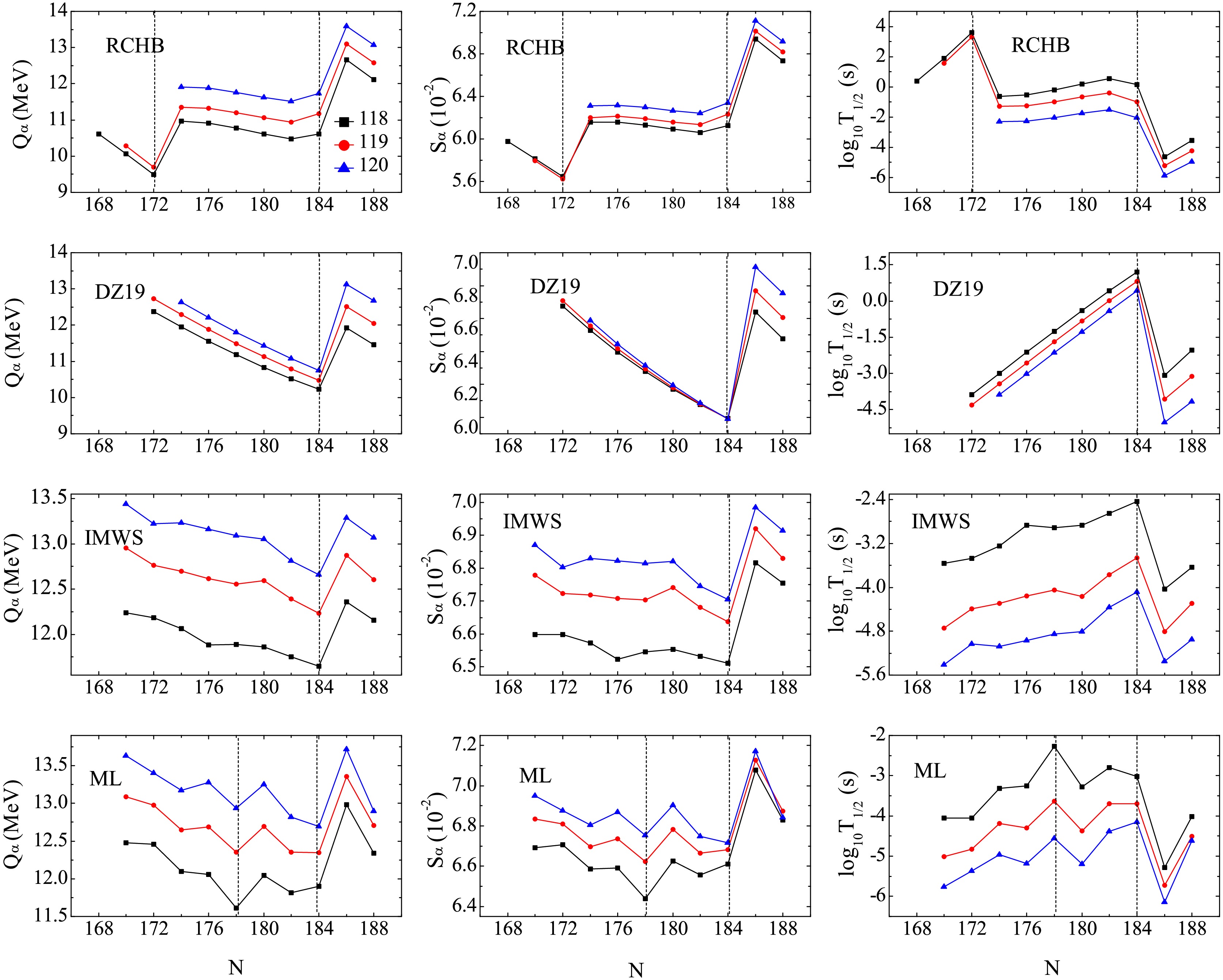
Figure 4. (Color online) Left panel: The extracted
$ Q_{\alpha } $ values of Z = 118-120 isotopes versus N for RCHB theory, DZ19, IMWS, and ML models. Middle panel: Same as the left panel, but for the corresponding$ S_{\alpha } $ values. Right panel: Same as the left and middle panels, but for the corresponding$ \log _{10}T_{1/2} $ values. -
In this article, the α-decay half-lives of SHN with Z≥104 have been calculated by the one-parameter model. By the comparison between the calculations and experimental data, it is shown that the calculated half-lives are in good agreement with the experimental data. Moreover, the
$S _{\alpha } $ values and α-decay half-lives of the Z = 118-120 isotopes are estimated by inputting the$ Q_{\alpha } $ values extracted from the RCHB, DZ19, IMWS and ML nuclear mass tables. It is shown that the order of magnitude of$S _{\alpha } $ is$ 10^{-2} $ . By analyzing the$ Q_{\alpha } $ values, the corresponding$S _{\alpha } $ and$ \log _{10}T_{1/2} $ values versus the neutron number N, it is found that the shell effect at N = 184 is evident for all the cases. Meanwhile, it is found that N = 172 is the submagic number for the RCHB theory. However, the submagic number at N = 172 is replaced by N = 178 for the ML approach. We hope our study is helpful for the synthesis of the new SHN in the future. At last, it is necessary to point out that the two-proton radioactivity, especially for its spectroscopic factor, has been an attracted subject in recent years [88−91]. However, it is a challenging task to obtain the accurate spectroscopic factor because the correlation between the two emitted protons is complex [88−93]. So it is interesting to extend or improve the one-parameter model to extract the spectroscopic factor of the two-proton radioactivity, which is a work in progress.
α-decay half-lives of superheavy nuclei within a one-parameter model
- Received Date: 2025-04-12
- Available Online: 2025-10-01
Abstract: The α-decay half-lives of superheavy nuclei (SHN) with charge number Z≥104 are investigated by employing a phenomenological one-parameter model based on the quantum-mechanical tunneling through a potential barrier where both the centrifugal and overlapping effects have been taken into account. It is shown that the experimental α-decay half-lives of the 81 SHN are reproduced well. Moreover, the order of magnitude for the α-particle preformation probability inside a parent nucleus (


 DownLoad: