


 Abstract
 HTML
HTML Reference
 Related
 PDF
PDF


-
Studying the movement of particles near black hole (BH) models is a genuinely intriguing subject in the vicinity of astrophysics and general relativity (GR) [1−3]. This fascination arises from intense scenarios found around BHs, offering a distinct setting to confirm Einstein's theory of GR. Furthermore, close to the boundary of a BH, the strong gravitational force distorts the paths of particles and nearby matter and light because of its intensity [4]. Near a BH, particles can explain different movements based on their starting conditions and BH characteristics such as its mass, charge, and angular momentum [5−7]. Particles can either be in stable or unstable orbit, move towards the BH in a spiral, or move away from it infinitely. Analyzing these paths offers better information, showing spacetime properties near BHs [8–9]. Remarkably, equations overseeing particle movement obtained from geodesic equations in a curved spacetime suggest that the nearer a particle approaches the event horizon [10−12], the greater is the impact of relativistic effects such as time dilation and gravitational redshift. These effects are most noticeable at the innermost stable circular orbit (ISCO), which is the nearest point a particle can orbit a BH without being sucked in [13]. Studying ISCO and other key orbits can aid in comprehending accretion mechanisms near BHs, which is essential for analyzing observational data from high-energy astrophysical events such as X-ray binaries and active galactic nuclei [14]. In this context, these works have important consequences for spotting gravitational waves produced by the merging of binary BHs because the motions of particles in intense gravitational fields strongly affect the inspiral and merger phases [15−20]. Primary frameworks for developing an understanding of these dynamics are provided by theoretical models such as those proposed by Kerr [21] and Schwarzschild [22]. Observational validations such as those from the Event Horizon Telescope [23] have additionally supported these theoretical forecasts. Comprehending the movement of particles near BHs remains a key focus of theoretical studies and observational astrophysics. The effect of magnetic and brane characteristics on the effective potential of the radial motion of a charged test particle around a slowly rotating BH in a braneworld within a uniform magnetic field was analyzed [24] by using the Hamilton-Jacobi technique. Furthermore, literature has featured fascinating studies on particle motion near BHs [25−29]. One study [30] investigated the movement of test particles around three BHs in the Einstein-Maxwell-scalar theory. Another study [31] probed the rotation of test particles around a Schwarzschild-MOG BH. Orbits of neutral particles and photons, both massive and massless, circling regular BHs were examined by Fan and Wang [32].
The study of BH shadows and their optical properties has a long history. The idea of observing the shadow of a BH was first proposed by Synge [33]; subsequently, detailed investigations into the size of the shadow were performed by Luminet [34] and Bardeen [35]. Additionally, the shape and size of BH shadows within various gravitational theories have been extensively analyzed by many studies (see [34, 36−47]). The formation of a BH shadow is closely linked to the gravitational lensing effect predicted by general relativity, and it is important to note the considerable body of contemporary literature focusing on strong-field gravitational lensing (see [48−52]).
An alternative approach for investigating particle dynamics involves showing the motion of magnetized particles around BHs within an external magnetic field [53– 54]. In addition, the motion of such magnetized particles around non-Schwarzschild BHs has been explored [55]. The motion of particles around BHs under the effect of external fields has been an active area of research. A foundational study [56] tested the structure of external electric and magnetic fields around rotating and static BHs immersed in an asymptotically uniform magnetic field. Over the years, numerous works have expanded on this by investigating various properties of electromagnetic fields near BHs exposed to external magnetic fields and the intrinsic magnetic fields of rotating magnetized neutron stars exhibiting dipolar structures across different gravitational models [57−66]. Such electromagnetic fields significantly affect the dynamics of charged particles near BHs [67−74]. Beyond charged particles, studies have investigated how magnetic fields affect the motion of magnetized particles with intrinsic magnetic dipole moments. In addition, the behavior of these particles around rotating and non-rotating BHs within external magnetic fields has been studied in [53–54].
Studies on entropy in a BH are known to go against the second law of thermodynamics [75–76], potentially leading to a decrease in the overall entropy of the universe when an object with limited entropy enters the event horizon [8, 77]. In this context, where BHs are believed to possess the highest possible amount of entropy compared to that of any other item of the same size [78−80], with this maximum entropy increasing about the surface area of the BH, the relationship
$ S = {A}/{4} $ is crucial for establishing the holographic principle [81–82] and is a common feature in most quantum gravity theories. However, the entropy-area relationship is likely to be altered by quantum fluctuations [83], especially as BHs emit Hawking radiation and decrease in mass [84]. Different methods such as non-perturbative quantum GR have shown that primary adjustments to BH entropy follow a logarithmic pattern [85]. These adjustments have been validated in numerous settings, such as by using the Cardy formula, analyzing BTZ BHs [84], studying matter fields in BH environments [86−93], and exploring string theory, all of which indicate that BH entropy is impacted by logarithmic corrections [94].The greybody factor (GF) is an important model in the study of BH physics, particularly in Hawking radiation (HR). It represents the probability that a wave originating from infinity will be absorbed by the BH, which is often referred to as the rate of absorption probability. As HR travels through the curved spacetime geometry around the BH model, the surrounding spacetime acts as a radiation barrier, significantly altering the observed black-body radiation spectrum. Furthermore, this modification necessitates calculating the greybody factor to use the transmission amplitude of the radiation of the BH. The GF is directly connected to the absorption cross section, which quantifies the likelihood of absorption. Various methods are employed to compute the greybody factor, which includes the matching method, rigorous bound method, WKB approximation, and analytical techniques for different spin fields. Extensive literature and topical reviews are available to guide researchers in these calculations, making the greybody factor a well-studied yet continually evolving aspect of BH thermodynamics and quantum field theory in curved spacetime [95−115].
Sakharov [116] and Gliner [117] showed that BH singularities can be avoided with a de Sitter core (
$ p = -\rho $ ), leading Bardeen [118] to propose a singularity-free "regular BH" solution with well-behaved spacetime at$ r = 0 $ . Beato and Garcia [119] subsequently derived the exact form of the Bardeen solution. Bronnikov [120–121] provided a key insight, which shows that the regularity of these BHs requires a nonlinear electrodynamics (NED) charge to manifest as a magnetic monopole. Since then, considerable research has explored regular BHs as the exact solutions of GR coupled with NED [122−133]. Hayward [134] introduced a new regular spacetime defined by the spherically symmetric metric:$ \begin{aligned}[b]\mathrm{d}s^2=\; & -\left(1-\frac{2mr^2}{r^3+2\ell^2m}\right)\mathrm{d}t^2+\left(1-\frac{2mr^2}{r^3+2\ell^2m}\right)^{-1}\mathrm{d}r^2 \\ & +r^2\left(\mathrm{d}\theta^2+\sin^2\theta\, \mathrm{d\mathrm{\mathrm{ }}}\phi^2\right),\end{aligned} $

(1) where m is used as a notation for the BH mass and
$ \ell $ represents a fundamental length scale. At large distances, this solution behaves like the Schwarzschild metric, whereas at small distances, it transitions to an anti-de Sitter (AdS) vacuum. Derived by coupling GR with NED (where the magnetic charge g satisfies$ g^3 = 2m \ell^2 $ ). In this context, the Hayward solution was widely studied over the last two decades because of its analytical simplicity and physical significance [135−146].This study tested the behavior of Hayward-Letelier BHs in the AdS space model, specifically looking at their unique properties and the impact of the cosmological constant in AdS setups. Furthermore, the metric function
$ f(r) $ is determined by the Hayward parameter g, the mass term M, the cosmological constant L, and an extra parameter α that causes significant changes to the geometry of the BH.We tested particle dynamics by studying the effective potential
$ V_{\text{eff}} $ model (e.g., many studies [147−157] illustrated the effective potential$ V_{\text{eff}} $ ) and focused on the ISCOs and photon sphere radius$ r_{ph} $ parameters as key features of null geodesics. In addition, we tested how BH shadows depend on parameters L, g, and α. Moreover, we studied the thermodynamic properties of the system by evaluating the Hawking temperature$ T_H $ and analyzing how variables L, r, and g affect the thermal behavior of BHs.The rest of this manuscript is organized as follows: Section II focuses on the dynamics of the Hayward-Letelier BHs in AdS spacetime, where we study the thermodynamic temperature (IIA) and thermal fluctuations (IIB). The final section (VI) presents the conclusion and summary. We use a system of units in which
$ G = c =1. $ -
The line element of Hayward-Letelier BHs in AdS spacetime is given by [158]:
$ \begin{aligned}[b] & \mathrm{d}s^2=-f(r)\mathrm{d}t^2+f(r)^{-1}\mathrm{d}r^2+\mathrm{d}\cal{P}^2, \\ \text{with}\quad & \mathrm{d}\cal{P}^2=r^2\left(\mathrm{d}\theta^2+\mathrm{sin}^2\theta\mathrm{d}\phi^2\right),\end{aligned} $

(2) where
$ f(r)=1 -\frac{2 M r^2}{g^3+r^3}+\frac{r^2}{L^2}-\alpha. $

(3) where α represents the cloud of string parameters, integration constant M is interpreted as the mass of BH, g represents the magnetic charge, and
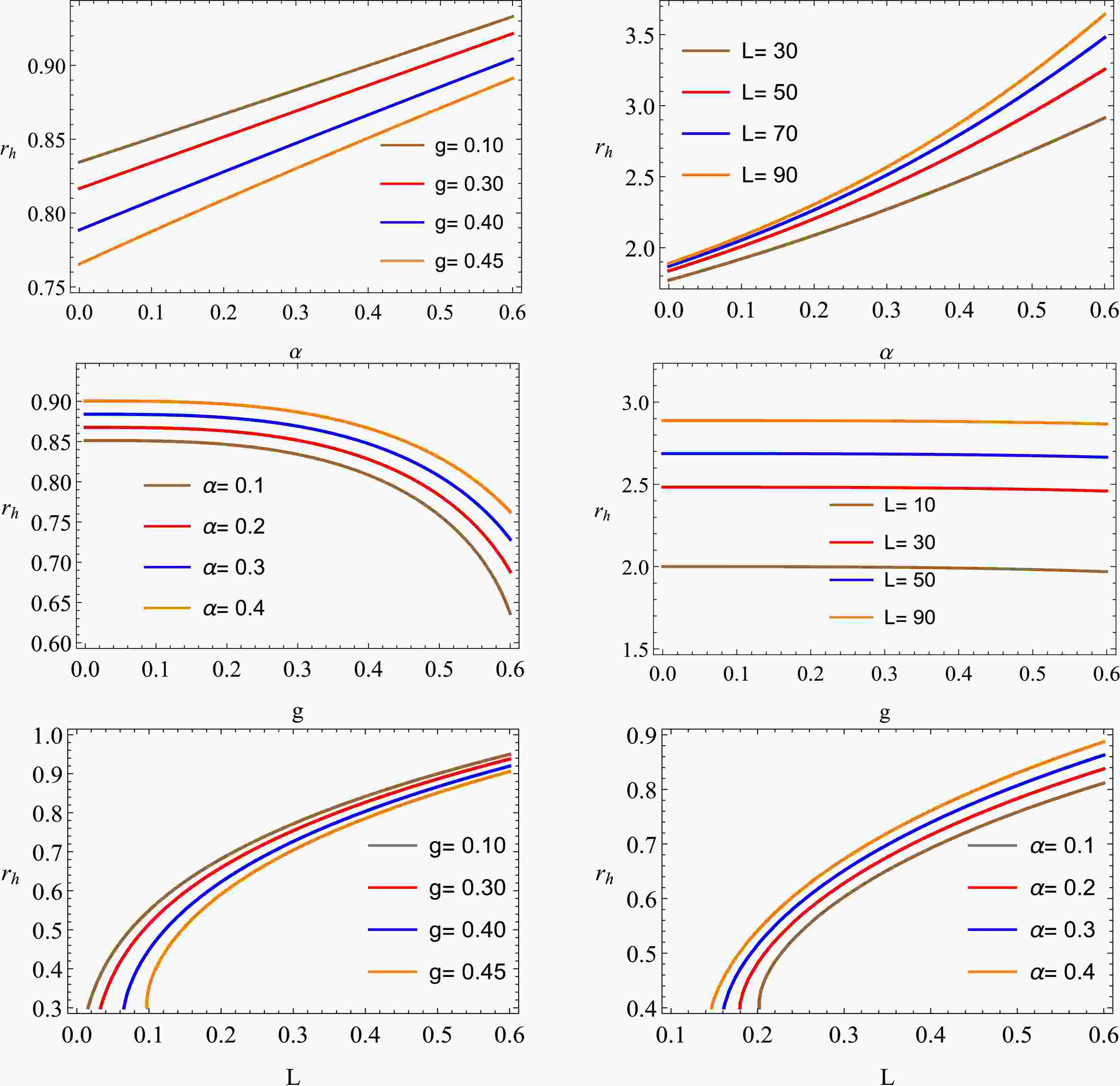
$ L>0 $ represents the AdS radius, which is related to the cosmological constant Λ. In the entire discussion, we use the relationship$ \Lambda =-3/L^2 $ . We analyze the possible existence of the horizon radius$ r_h $ by graphical analysis as shown in Fig. 1. It is seen that$ r_h $ along α reduces with an increase in g and increases with an increase in L. In addition,$ r_h $ along g increases with rising α and L. Furthermore,$ r_h $ along L reduces with an increase in g and rises with an increase in α.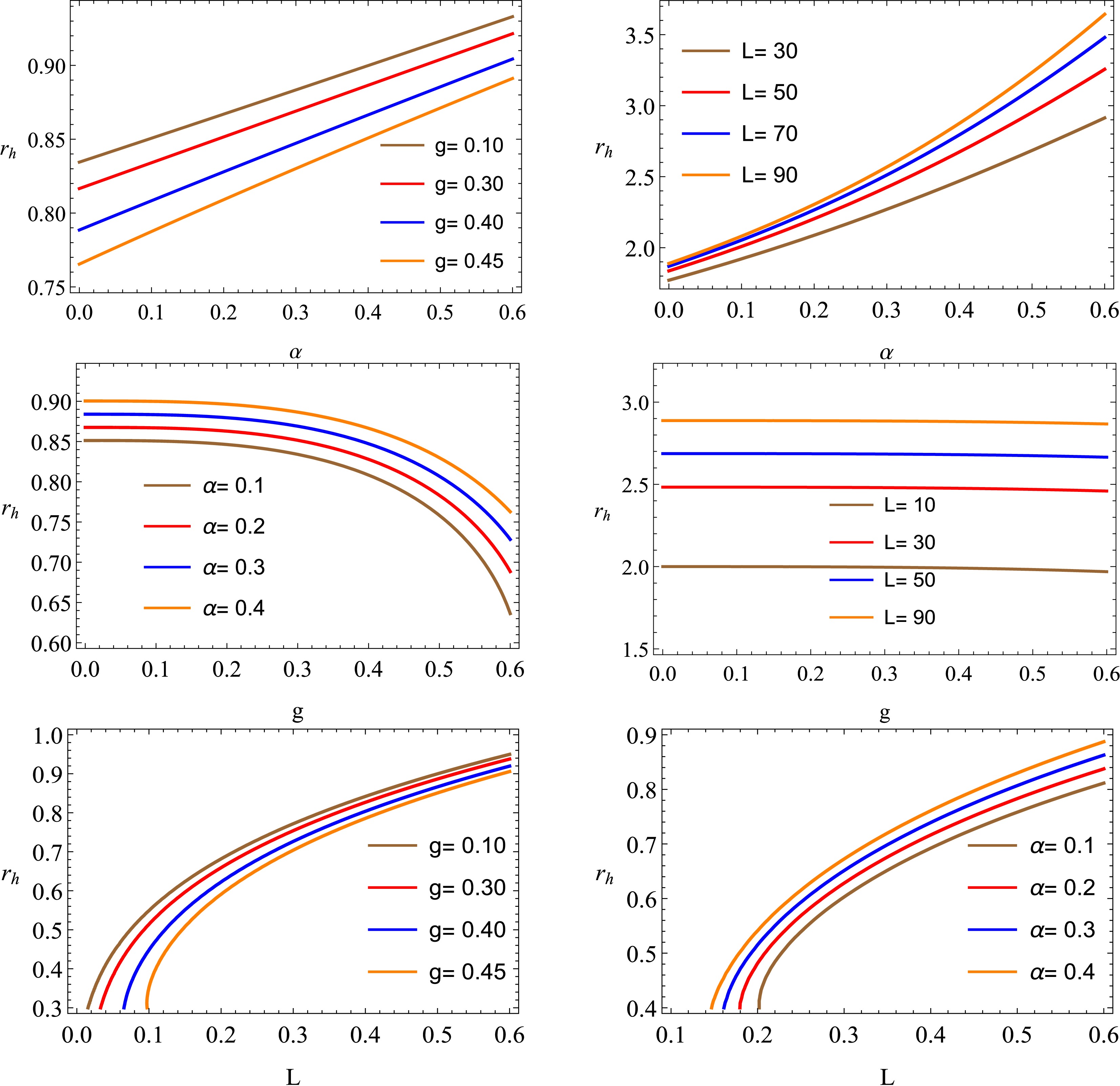
Figure 1. (color online) Horizon radius
$ r_h $ .We start by analyzing the motion of massive particles within the framework of the Hayward-Letelier BH in AdS spacetime. To characterize the trajectory of this motion, we use the Lagrangian for a massive particle of mass M given by [159]:
$ {\cal{L}}'=\frac{1}{2}g_{\mu\nu}u^{\mu}u^{\nu},\; \; \; u^{\mu}=\frac{\mathrm{d}x^{\mu}}{\mathrm{d}\tau}. \;\;\;$

(4) By using the process given in [28, 159], we can find effective potential:
$ V_{\mathrm{eff}}(r)=f(r)\cal{F}, $

(5) where
$ {\cal{F}}=\left(1+\frac{{\cal{L}}^2}{r^2}\right). $

(6) In this context,
$ V\mathrm{_{\mathrm{eff}}}(r) $ and$ {\cal{L}} $ represent notations used for the effective potential defining the motion of the test particle along the radius and angular momentum, respectively. The motion of neutral particles around the BH may be determined by setting$ \dot{r} = 0 $ and$ \ddot{r} = 0 $ .Next, we examine the
$ \mathrm{ISCO} $ radius$ r_{\mathrm{ISCO}} $ . To find$ r_{\mathrm{ISCO}} $ , the following conditions can be applied:$ \left\{\begin{array}{l} V_{\mathrm{eff}}'=0, \\ V_{\mathrm{eff}}{''}=0.\end{array}\right. $

(7) We plot the
$ \mathrm{ISCO} $ radius$ r_{\mathrm{ISCO}} $ in Fig. (2).$ r_{\mathrm{ISCO}} $ along α decreases by increasing g and increases by increasing L,$ r_{\mathrm{ISCO}} $ along g increases by increasing$ \alpha\;\&\;L $ , and$ r_{\mathrm{ISCO}} $ along L decreases by increasing g and increases by increasing α.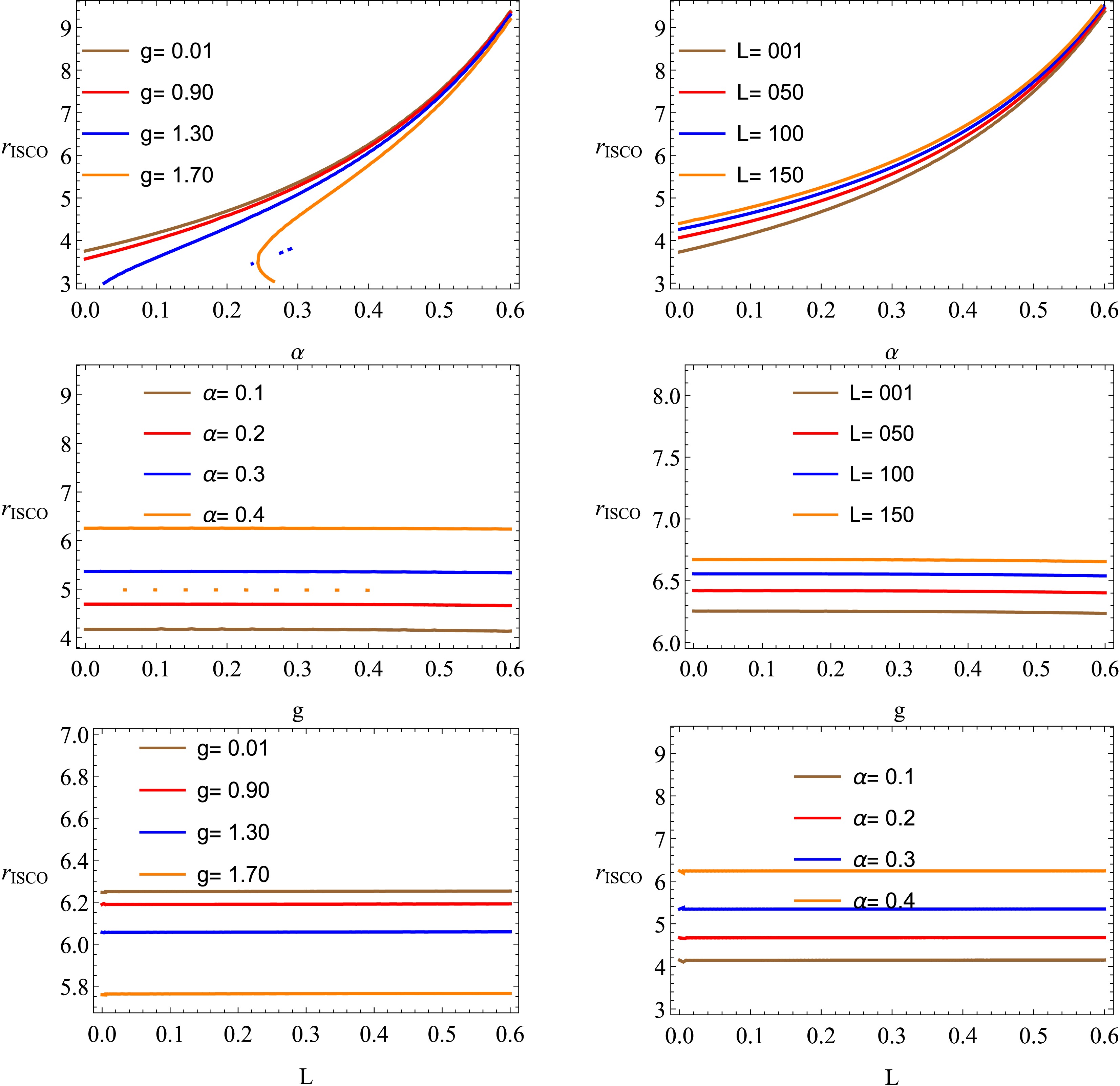
Figure 2. (color online) ISCO radius.
Now, we analyze the motion of massless particles (photons) using the spacetime of a BH in the context of Hayward-Letelier BHs in AdS spacetime. Using the procedure given in [28, 159], we can find the effective potential for photon motion:
$ V_{\mathrm{eff}}=f(r)\frac{\cal{L}^2}{r^2}. $

(8) The photon's radius
$ r_{ph} $ in Hayward-Letelier BHs in AdS spacetime could be evaluated by solving Eq. (7) along with Eq. (2). The solution is complex, and therefore a numerical method is used to plot$ r_{ph} $ directly without deriving its explicit expression. The shift in the photon orbit radius is illustrated in Fig. (3). The photon radius$ r_{ph} $ along α decreases with an increase in g, and$ r_{ph} $ along g increases with an increase in α. It is important to note that the expression calculating the photon radius$ r_{ph} $ is independent of L, and therefore there is no relative change in$ r_{ph} $ with L.
Figure 3. (color online) Photon
$ r_{ph} $ radius.Analysis of BH shadows provides valuable information related to the apparent diameter of the event horizon and can reveal insights into the spin of the BH and accretion disk orientation. In studying these shadows, GR is tested in extreme gravity environments, offering insights into the astrophysical properties and evolution of BHs. Advances in observational methods such as very long baseline interferometry (VLBI) have enhanced our ability to resolve and study these shadows with greater precision, opening new opportunities for investigating BHs and their surrounding environments. We study the shadows of the BH in Hayward-Letelier gravity, which is determined by [160]:
$ {\rm{sin}}^2\left(\alpha_{s h}\right)=\frac{r_{p h}^2}{f\left(r_{p h}\right)} \frac{f\left(r_o\right)}{r_o}.$

(9) Utilizing the small-angle approximation, the size of the shadow can be determined as [160]:
$ r_{s h}=r_{p h} \sqrt{\frac{f\left(r_o\right)}{f\left(r_{p h}\right)}}. $

(10) Eq. (10) defines the non-rotating case for BH shadows, which we plot in Figs. 4 and 5. The BH shadow radius
$ R_{sh} $ can be represented by the two celestial coordinates X and Y, where$ R_{sh} = \sqrt{X^2 + Y^2} $ for the observer [161–162]. It is noted that the shadow radius behaves very similarly to the$ r_{\mathrm{ISCO}} $ radius. The shadow radius$ R_{sh} $ along α decreases with an increase in g and increases with an increase in L;$ R_{sh} $ along g increases with an increase in$ \alpha\;\&\;L $ ; and$ R_{sh} $ along L decreases with an increase in g and increases with an increase in α.
Figure 4. (color online) Shadows radius
$ R_{sh} $ .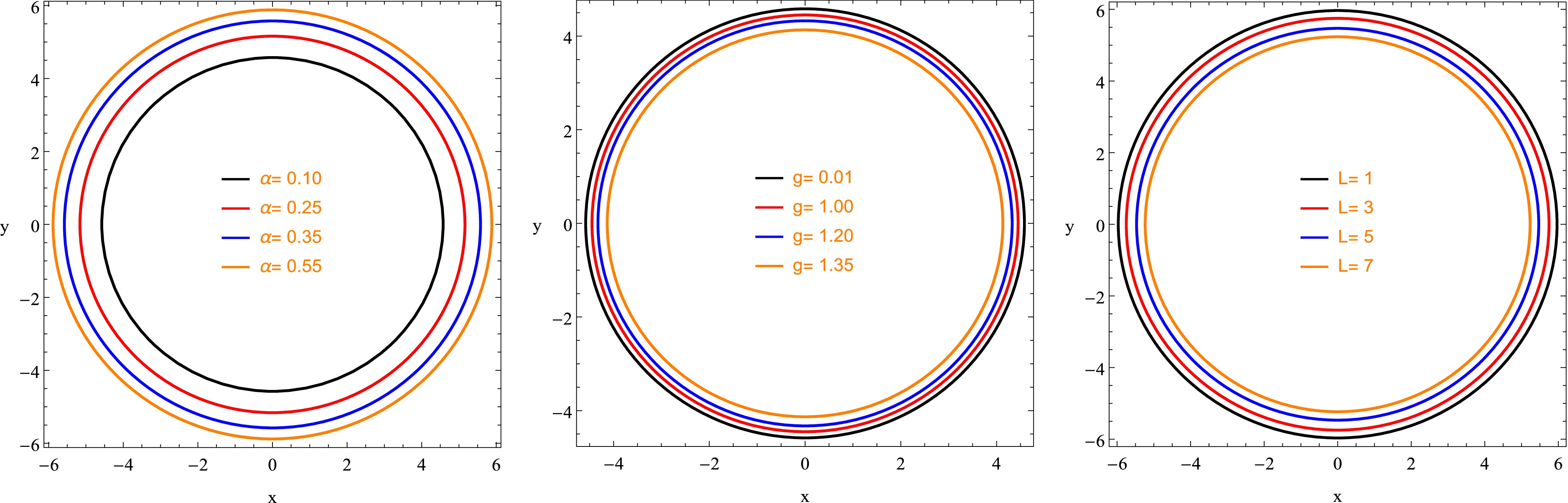
Figure 5. (color online) Shadows radius
$ R_{sh} $ . -
Differentiating function
$ f(r) $ with respect to the radial coordinate r yields the thermodynamic temperature$ T_H $ of the BH, as expressed in the following equation:$\begin{aligned}[b]\\[-4pt] T_H = \frac{1}{4 \pi} \frac{\partial f(r)}{\partial r} = \frac{r{\cal{K}}(r_{0},g,L)}{2 \pi}, \end{aligned}$

(11) where
$ {\cal{K}}(r_{0},g,L)=\left( \frac{M (r_{0}^3 - 2 g^3)}{(g^3 + r_{0}^3)^2} + \frac{1}{L^2} \right). $

(12) Here,
$ r_0 $ represents the horizon radius of the BH.● This equation yields the temperature at the event horizon of the BH, which is an important thermodynamic parameter. The temperature is determined by the mass M of the BH, along with factors g and L, and the radial distance r from the center. The effect of the AdS parameter L has a characteristic effect from the curvature of spacetime that affects temperature.
Furthermore, the BH entropy S can be described using the entropy equation, as demonstrated in [163]:
$ S = \frac{1}{\kappa} \log \left( 1 + \pi \kappa r_{0}^2 \right), $

(13) where κ represents a fixed value associated with the characteristics of the BH. The entropy equation represents the amount of information in a BH and how it relates to the radius of horizon r. This logarithmic relationship shows how entropy increases with an increase in the size of the BH.
● The thermodynamic temperature plays a key role, and thus illustrating and showing the thermal properties of the BH is crucial. A greater temperature reflects a higher level of energy in the BH, which potentially affects how it emits radiation and interacts with its environment. To calculate temperature, this study considers the mass of the BH and curvature of spacetime, indicating that the cosmological constant (denoted by L) plays a major role in determining the thermodynamic characteristics of the AdS BHs.
● Furthermore, the entropy formula indicates the connection between the entropy of a BH and the area of its event horizon. The equation shows that entropy rises with the square of the horizon radius, which shows that bigger BHs possess more entropy. This is in agreement with the common belief that the entropy of the BH is directly related to the size of the event horizon, as explained by the Bekenstein-Hawking entropy equation.
● The relationship between temperature, entropy, and various parameters of a BH, such as mass M, AdS parameter L, and radial coordinate r, reveals complex thermodynamic connections within the system. Understanding the stability and evolution of BHs, especially in the AdS spacetime, relies on these crucial relationships influenced by cosmological effects shaping the properties of the BH.
-
In this part, we study how thermal fluctuations affect the thermodynamics of the recently suggested BH model. To examine this effect, we employ the Euclidean quantum gravity framework in which the time axis is shifted into the complex plane. This method enables us to specify the partition function for the BH, as detailed in [164−169]. For a more in-depth explanation, consult [165], which summarizes a simplified procedure
$ Z=\int D g D A \exp (-I). $

(14) The expression
$ I \rightarrow \iota \hat{I} $ represents the Euclidean action of the field in this context, where the integral runs over all fields that adhere to specific periodicity or boundary conditions. The statistical mechanical partition function is related to [170–171]:$ Z=\int_0^{\infty} D E \Gamma(E) \exp (-\psi E), $

(15) where ψ represents the reciprocal of T. The density of states can be obtained through
$ \Gamma(E)=\frac{1}{2\pi\mathrm{i}}\int_{\psi_0-\mathrm{i}\infty}^{\psi_0+\mathrm{i}\infty}\mathrm{d}\psi\mathrm{e}^{S(\psi)}, $

(16) $ S_c $ represents the sum of$ \psi E $ and natural logarithm of Z. Ignoring thermal fluctuations, the entropy near the equilibrium temperature ψ can be calculated as$ S = \delta \left(\pi r^2\right)^{\kappa} $ . However, when thermal fluctuations are considered, the entropy$ S_c(\psi) $ is given by [164]:$ S_c=S+\frac{1}{2}\left(\psi-\psi_0\right)\left(\frac{\partial^2 S(\psi)}{\partial \psi^2}\right)_{\psi=\psi_0}. $

(17) Thus, density can be expressed using
$ \Gamma(E)=\frac{1}{2\pi\mathrm{i}}\int_{\psi_0-\mathrm{i}\infty}^{\psi_0+\mathrm{i}\infty}\mathrm{d}\psi\mathrm{e}^{\frac{1}{2}\left(\psi-\psi_0\right)\left(\frac{\partial^2S(\psi)}{\partial\psi^2}\right)_{\psi=\psi_0}}, $

(18) and
$ \Gamma(E)=\frac{\mathrm{e}^S}{\sqrt{2\pi}}\left[\left(\frac{\partial^2S(\psi)}{\partial\psi^2}\right)_{\psi=\psi_0}\right]^{\frac{1}{2}}. $

(19) The corrected entropy equation can be expressed using
$ S_c=S-\frac{1}{2} \ln \left[\left(\frac{\partial^2 S(\psi)}{\partial \psi^2}\right)_{\psi=\psi_0}\right]^{\frac{1}{2}}. $

(20) The square of the energy fluctuation is expressed through the second derivative of entropy. This expression can be simplified by utilizing the connection between the conformal field theory and microscopic degrees of freedom of a BH [84]. Consequently, the entropy is given by
$ S = m_1 \psi^{n_1} + m_2 \psi^{-n_2} $ , where$ m_1 $ ,$ m_2 $ ,$ n_1 $ , and$ n_2 $ are positive constants [85].This entropy reaches its maximum at
$ \psi_0 = \left(\dfrac{m n_2}{m_1 n_1}\right)^{\frac{1}{n_1+n_2}} = T_H^{-1} $ , with$ T_H $ being the Hawking temperature defined in Eq. (11). Expanding the entropy around this peak leads to the results presented in [172–173]:$ \left(\frac{\partial^2 S(\psi)}{\partial \psi^2}\right)_{\psi=\psi_0}=S \psi_0^{-2} . $

(21) A revised expression for entropy obtained by excluding higher-order corrections is given by:
$ S_c=S-\frac{1}{2} \ln S T_H^2 . $

(22) The prevalence of quantum fluctuations in the shape of BHs raises important questions about thermal fluctuations generated in the case of BH thermodynamics. These fluctuations play an important role when the BH is small and has a high temperature. For larger BHs, quantum fluctuations may be neglected. Thermal fluctuations are only significant in BHs with high temperatures, and its temperature increases as the BH becomes smaller. Consequently, it can be concluded that these adjustment factors are relevant for very small BHs with high temperatures [164]. Afterward, we can derive the general formula for entropy by neglecting higher-order correction terms:
$ S_c=S-\gamma \ln S T^2. $

(23) In this context, we define γ as a fixed parameter that incorporates logarithmic correction terms associated with thermal fluctuations. When γ is set to zero, the entropy expression is obtained without any correction terms. As mentioned earlier, for large BHs with very low temperatures, we take
$ \gamma \rightarrow 0 $ , and for small BHs with high temperatures, we take$ \gamma \rightarrow 1 $ . Using Eqs. (11) and (23), we can derive the corrected entropy formula:$ S_c=\frac{\log \left(\pi \kappa r_{0}^2+1\right)}{\kappa }-\gamma \log \left({\cal{A}}\right), $

(24) where
$ {\cal{A}}=\frac{r_{0}^2 }{4 \pi ^2 \kappa }\log \left(\pi \kappa r_{0}^2+1\right) \left(\frac{M \left(r_{0}^3-2 g^3\right)}{\left(g^3+r_{0}^3\right)^2}+\frac{1}{L^2}\right)^2. $

(25) The value of
$ S_C $ is plotted for the different values of the correction parameter in Fig. (6), where$ \gamma=0 $ for large BHs, and$ \gamma=0.1,\; 0.4,\;0.7,\; \text{ and } \;1.0 $ for small BHs ($ 0 < \gamma < 1 $ ). One can see that, for large BHs, no fluctuations are observed. Moreover, corrected entropy increases by increasing parameters$ g,\;L,\;\kappa,\;\gamma $ , whereas no variations are observed for increasing values of α as the expression is independent of α.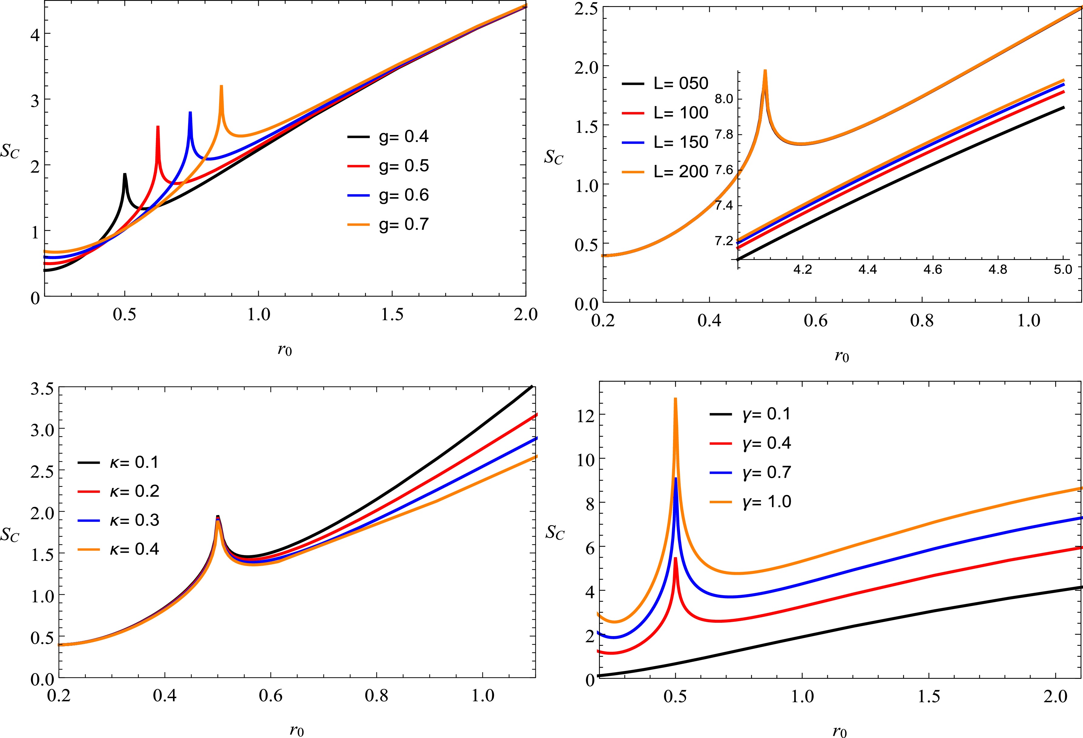
Figure 6. (color online) Thermal fluctuations
$ S_{c} $ . -
In this section, we compute the GBF analytically. First, we examine the equation of motion (EoM) to study the propagation of a massless scalar field, assuming that particles are only weakly coupled to gravity and do not exhibit additional interactions. Next, the EoM results in
$ \nabla_{\beta}\nabla^{\beta}\Psi=\partial_{\beta}[\sqrt{-g}g^{\beta\gamma}\partial_{\gamma}\Psi]=0, $

(26) in which the massless scalar field is presented by
$ \Psi=\Psi(t,r,\theta,\phi) $ . From Eq. (26), it is found that$\begin{aligned}[b]& \frac{-r^{2}\sin\theta}{f(r)}\partial_{tt}\Psi+\sin\theta \partial_{r} \bigg(r^{2} f(r)\partial_{r}\Psi\bigg)\\&\quad+\partial_{\theta} \bigg(\sin\theta\partial_{\theta}\Psi\bigg)+ \frac{1}{\sin\theta}\partial_{\phi\phi}\Psi =0, \end{aligned}$

(27) and through the separation of variables technique, one can get
$ \Psi=\exp(-\iota w t)\exp(\iota m\phi)R_{w l m}(r)Q^{m}_{l}(\theta,a w), $

(28) in which the angular spheroidal function is displayed by
$ Q^{m}_{l}(\theta,a w) $ . Equation (13) enables us to calculate the radial and angular components of the EoM as [174–175]$ \frac{\partial }{\partial r}\bigg[r^{2}f(r)\frac{\partial R_{w l m}}{\partial r}\bigg]+\bigg[\frac{r^{2}\omega^{2}}{f(r)}- \lambda^{m}_{l}\bigg]R_{w l m}(r)=0, $

(29) and
$ \frac{\partial}{\partial\theta}\bigg[\sin\theta\frac{\partial Q^{m}_{l}}{\partial\theta}\bigg]+\bigg[\frac{-m^{2}}{\sin\theta}+\lambda^{m}_{l}\sin\theta\bigg]Q^{m}_{l}(\theta,\alpha w)=0, $

(30) respectively. It is important to note that, in the following discussion, we use
$ \alpha=a $ in equation 3. The connection between decoupled equations is defined by the separation constant$ \lambda_{l}^{m} $ . Although$ \lambda_{l}^{m} $ cannot typically be expressed in a closed form, its analytical expression can be approximated in a series [174–175]. Now, we derive the precise solutions to the radial EoM (29). The obtained solution yields the GBF for a massless scalar field. We can examine the effective potential profile that describes the GBF by solving the radial equation. A new radial transformation is introduced as$ R_{wlm}(r)=\frac{U_{wlm}(r)}{r}. $

(31) By employing the tortoise constituent
$ x_{*} $ , we get$ \frac{\mathrm{d}x_*}{\mathrm{d}r}=\frac{1}{f(r)}, $

(32) which yields
$ \frac{\mathrm{d}}{\mathrm{d}x_*}=f(r)\frac{\mathrm{d}}{\mathrm{d}r}, $

(33) $ \frac{\mathrm{d}^2}{\mathrm{d}x_*^2}=f^2(r)\frac{\mathrm{d}^2}{\mathrm{d}r^2}+ff'\frac{\mathrm{d}}{\mathrm{d}r}. $

(34) As r approaches
$ r_{h} $ ,$ x_{*} \rightarrow -\infty $ , and as$ r \to \infty $ ,$ x_{*} \rightarrow \infty $ . The tortoise coordinates$ x_{*} $ transform the range of the model from$ -\infty $ to$ +\infty $ , in contrast to Eq. (29), which is restricted to regions far from the BH horizon. Equation (29) can be recognized as a Schrödinger wave equation expressed as$ \left(\frac{\mathrm{d}^2}{\mathrm{ }\mathrm{d}x_*^2}-V_{\mathrm{eff}}\right)U_{wlm}(r)=0. $

(35) The associated form of the effective potential leads to
$ V\mathrm{_{eff}}=-\omega^2+\frac{ff'}{r}+\frac{\lambda_l^mf(r)}{r^2}. $

(36) The profile of the effective potential in view of the varying values of BH charge as a function of BH cloud of strings parameter is shown in Fig. 7. The potential decreases by increasing the cloud of strings parameters. Additionally, the effective potential decreases with increasing g. Furthermore, we observe the effect of BH mass on the effective potential by varying the cloud of strings parameter as shown inFig. 8. The effective potential increases for massive BHs.
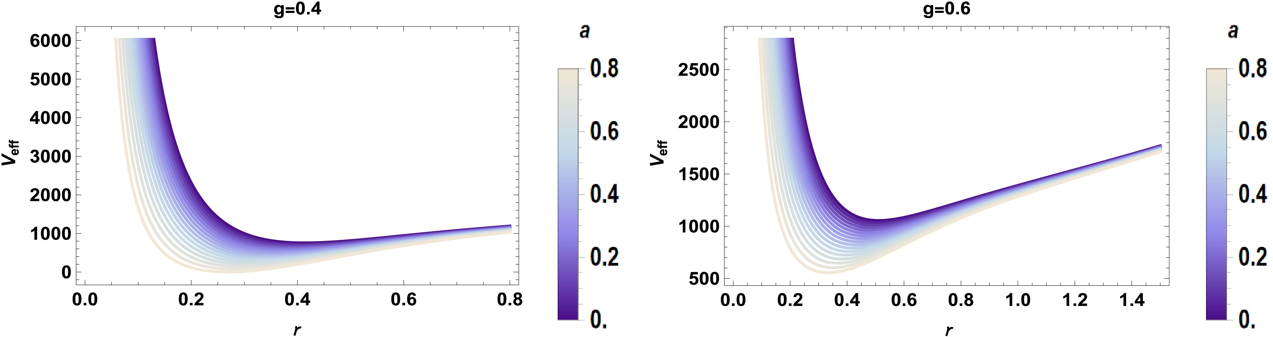
Figure 7. (color online)
$ V_{eff} $ versus$ r_h $ by varying a and g.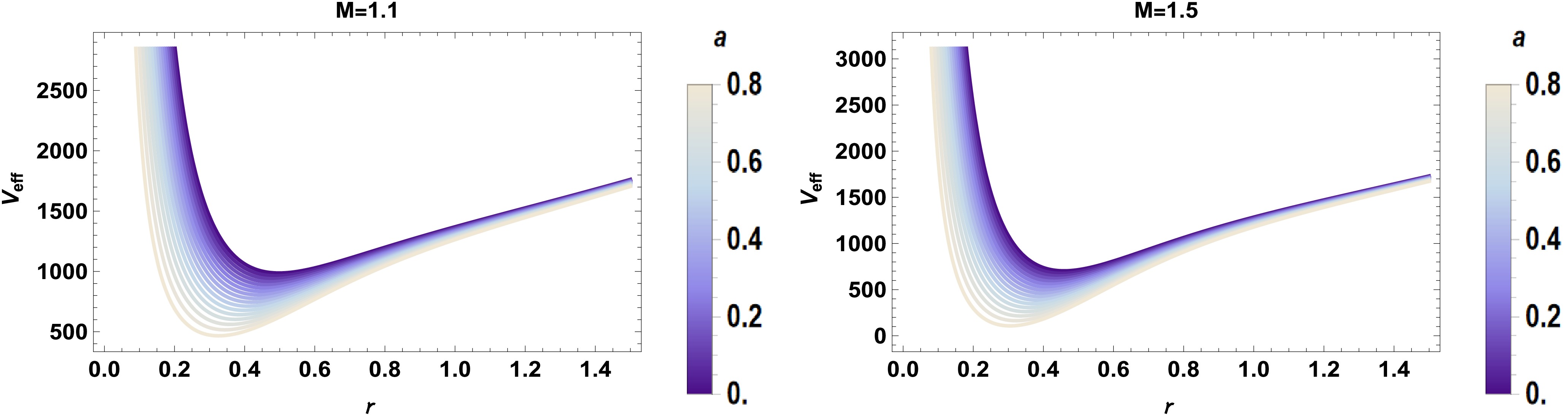
Figure 8. (color online)
$ V_{eff} $ versus$ r_h $ by varying a and M. -
This section suggests analytical solutions to GBF, which results from the equation explaining the radial motion (29). We find two asymptotic solutions for distinct modes, e.g., close to and far away from the BH event horizon. To arrive at the solutions for the entire area, we contrast these solutions uniformly in an intermediate domain. We apply the following transformation to obtain the analytical solution for the near horizon region
$ r\sim r_{h} $ $ r\rightarrow S=\frac{1-\dfrac{2Mr^2}{g^3+r^3}-a+\dfrac{r^2}{L^2}}{1-a+\dfrac{r^2}{L^2}}, $

(37) which yields
$ \frac{\mathrm{d}S}{\mathrm{d}r}=\frac{(1-S)U(r_h)}{r_h}, $

(38) and therefore, we have
$ U(r_{h})= \frac{\dfrac{2r^2}{L^2}-\dfrac{2g^3-r^3}{g^3+r^3}\bigg[1-a+\dfrac{r^2}{L^2}\bigg]}{1-a+\dfrac{r^2}{L^2}}. $

(39) Based on these results, the radial equation (29) can be expressed as
$\begin{aligned}[b]& S(1-S)\frac{{\rm d}^{2}R_{w l m}}{{\rm d} S^{2}}+(A-BS)\frac{{\rm d}R_{w l m}}{{\rm d} S}\\&\;\;+ \frac{1}{(1-S)U^{2}}\bigg[\frac{\chi_{h}}{S}-\lambda_{h}\bigg]R_{w l m}=0,\end{aligned} $

(40) where
$ \begin{aligned}[b] A =\;&\frac{r_h}{(1-S)U(r_{h})}\frac{\rm d}{{\rm d}r}(S-S^{2}),\\ B=\;&-\frac{S}{U^{2}(r_{h})\bigg[1-a+\dfrac{r^2}{L^2}\bigg]}\frac{\rm d}{{\rm d}r}\bigg[r_{h}U(r_{h}) \bigg(1-a+\frac{r^2}{L^2}\bigg)\bigg],\\ \chi_{h} =\;&\frac{w^{2}r^{2}_{h}}{\bigg[1-a+\dfrac{r^2}{L^2}\bigg]^2},\quad \lambda_{h}= \frac{\lambda^{m}_{l}}{1-a+\dfrac{r^2}{L^2}}. \end{aligned} $

(41) We re-express the function in Eq. (40) as
$ R_{w l m}(S)=S^{\epsilon_{1}}(1-S)^{\eta_{1}}\hat{F}(S). $

(42) Thus, the following expression of Eq. (40) is obtained.
$ \begin{aligned}[b]& S(1-S)\frac{{\rm d}^{2}\hat{F}(S)}{{\rm d} S^{2}} + \bigg[2\epsilon_{1}+A-(2\epsilon_{1}+2\eta_{1}+B)S\bigg]\frac{{\rm d} \hat{F}(S)}{{\rm d} S}\\&\;\;+ \bigg[\bigg(\epsilon^{2}_{1}-\epsilon_{1}+ A\epsilon_{1}+\frac{\chi_{h}}{U^{2}} \bigg)\frac{1}{S}+ \bigg(\eta^{2}_{1}-\eta_{1}-\eta_{1}A+\eta_{1}B\\&\;\;+ \frac{\chi_{h}}{U^{2}}-\frac{\lambda_{h}}{U^{2}}\bigg)\frac{1} {1-S}\bigg]\hat{F}(S)=0. \end{aligned} $

(43) The power coefficients
$ \epsilon_{1} $ ,$ \eta_{1} $ can be found, for example, by$ \begin{array}{l} \epsilon^{2}_{1}-\epsilon_{1}+A\epsilon_{1}+\dfrac{\chi_{h}} {U^{2}}=0,\\ \eta^{2}_{1}-\eta_{1}-\eta_{1}A+\eta_{1}B+\dfrac{\chi_{h}} {U^{2}}-\dfrac{\lambda_{h}}{U^{2}}=0.\end{array} $

(44) Finally, Eq. (43) is solved to attain the HG of the differential equation provided by
$ S(1-S)\frac{{\rm d}^{2} \hat{F}(S)}{{\rm d} S^{2}}+\bigg[\bar{c}_{1}-(\bar{a}_{1}+\bar{b}_{1}+1)S\bigg]\frac{{\rm d} \hat{F}(S)}{{\rm d} S}-\bar{a}_{1}\bar{b}_{1}\hat{F}(S)=0, $

(45) with
$ \bar{a}_{1}=\eta_{1}+\epsilon_{1}+B-1,\quad\bar{b}_{1}=\eta_{1}+ \epsilon_{1},\quad\bar{c}_{1}= 2\epsilon_{1}+A. $

(46) For NH, its general solution can be displayed as
$\begin{aligned}[b] (R_{w l m})_{NH}(S)=\;& \hat{A_{1}}S^{\epsilon_{1}}(1-S)^{\eta_{1}}\hat{F}(\bar{a}_{1},\bar{b}_{1},\bar{c}_{1} ; S )\\&+\hat{A_{2}}S^{-\epsilon_{1}}(1-S)^{\eta_{1}} \hat{F}(1-\bar{c}_{1}+\bar{a}_{1},\\& 1+\bar{b}_{1}-\bar{c}_{1},-\bar{c}_{1}+2;S),\end{aligned} $

(47) with
$ \hat{A_{1}} $ and$ \hat{A_{2}} $ as constants having$ \begin{align} \epsilon^{\pm}_{1} =& \frac{1}{2}\bigg[(1-A)\pm\sqrt{(1-A)^{2}-4 \frac{\chi_{h}}{U^{2}}}\bigg],\\ \eta^{\pm}_{1} =&\frac{1}{2}\bigg[(1+A-B)\pm\sqrt{(1+A-B)^{2}+4\bigg( \frac{\lambda_{h}}{U^{2}}-\frac{\chi_{h}}{U^{2}}\bigg)}\bigg]. \end{align} $

(48) We found that no outward modes exist at the BH horizon when applying the boundary conditions. We can choose to set
$ \hat{A_1} = 0 $ ; if this is not the case, then$ \hat{A_2} = 0 $ . This choice depends on the selection of$ \epsilon_1 $ . Since$ \hat{A_1} $ and$ \hat{A_2} $ are constants for both values of$ \epsilon_1 $ , we can conclude that$ \epsilon_1^+ = \epsilon_1^- $ by setting$ \hat{A_2} = 0 $ . Another approach to determine the signs of$ \eta_1 $ is using the convergence condition of the HG function, which holds when$ \eta_1^+ = \eta_1^- $ . Therefore, the analytic form of the near-horizon (NH) solution is expressed as$ (R_{w l m})_{N H}(S)=\hat{A_{1}}S^{\epsilon_{1}}(1-S)^{\eta_{1}} \hat{F}(\bar{a}_{1}, \bar{b}_{1},\bar{c}_{1};S). $

(49) We use the same approach as for the near-horizon solution to obtain the solution of the radial equation for the far BH horizon, which replaces
$ f(r) $ with$ T(r) $ as$ T(r)=\frac{1-a+\dfrac{r^2}{L^2}}{r^{2}}. $

(50) This yields the change in the radial equation as
$\begin{aligned}[b]& T(1-T)\frac{{\rm d}^{2} R_{ w l m}}{{\rm d}T^{2}}+(C-D^{\ast}T)\frac{{\rm d} R_{ w l m}}{{\rm d} T}\\&\;\;+\frac{1}{\dfrac{4(a-1)^2}{r^4}(1-T)}\bigg[\frac{\chi_{f}}{T}-\lambda_{f} \bigg] R_{ w l m}=0,\end{aligned} $

(51) where
$ \begin{aligned}[b] \chi_{f} =&\left(\frac{r w T(1-T)}{f(r)}\right)^2, \quad\lambda_{f}=\frac{\lambda_{l}^{m}T(1-T)^2}{f(r)},\\ C =&\frac{1-a+\dfrac{r^2}{L^2}}{\dfrac{4(a-1)^2}{r^3}f(r)}\frac{\rm d}{{\rm d}r}\bigg[\frac{2(a-1)}{r^2}f(r)\bigg], \\D^{\ast}=&\frac{1-a+\dfrac{r^2}{L^2}}{2(a-1)}.\end{aligned}$

(52) It is necessary to redefine the field in the differential equation mentioned above as
$ R_{wlm}(T)=T^{\epsilon_{2}}(1-T)^{\eta_{2}}\hat{F(T)}, $

(53) and we get
$ \begin{aligned}[b] & T(1-T)\frac{{\rm d}^{2}\hat{F(T)}}{{\rm d} T^{2}}+\bigg[ 2\epsilon_{2} + C - (2\epsilon_{2}+2\eta_{2} + D^{\ast})T\bigg]\frac{{\rm d} \hat{F(T)}}{{\rm d} T}\\&\;\; +\bigg[\bigg(\epsilon^{2}_{2}-\epsilon_{2} +\epsilon_{2}C+ \frac{\chi_{f}}{\dfrac{4(a-1)^2}{r^4}}\bigg)\bigg( \eta_{2}^{2}-\eta_{2}-\eta_{2}C+\eta_{2} D^{\ast} \\&\;\;+ \frac{\chi_{f}}{\dfrac{4(a-1)^2}{r^4}}-\frac{\lambda_{f}}{\dfrac{4(a-1)^2}{r^4}} \bigg)\frac{1}{1-T}\bigg]\hat{F(T)}=0. \\[-12pt]\end{aligned}$

(54) We obtain the power coefficients
$ \epsilon_{2} $ and$ \eta_{2} $ as$ \begin{array} {l}\epsilon^{2}_{2}-(1-C)\epsilon_{2}+\dfrac{\chi_{f}}{\dfrac{4(a-1)^2}{r^4}}=0,\\ \eta^{2}_{2}-(1-D^{\ast}+C)\eta_{2}+\dfrac{\chi_{f}} {\dfrac{4(a-1)^2}{r^4}}-\dfrac{\lambda_{f}}{\dfrac{4(a-1)^2}{r^4}}=0.\end{array} $

(55) Hence, the HG-based equation computed as
$ \bar{a}_{2}=\epsilon_{2}+\eta_{2}+D^{\ast}-1,\quad\bar{b}_{2}= \epsilon_{2}+\eta_{2},\quad\bar{c}_{2}= 2\epsilon_{2}+C, $

(56) becomes
$ T(1-T)\frac{{\rm d}^{2}\hat{F(T)}}{{\rm d} T^{2}}+ \bigg[\bar{c}_{2}-(1+\bar{a}_{2}+\bar{b}_{2})\bigg]\frac{{\rm d} \hat{F(T)}}{{\rm d} T}-\bar{a}_{2}\bar{b}_{2} \hat{F(T)}=0. $

(57) Its general solution is
$\begin{aligned}[b] (R_{wlm})_{f}(T)=\;& \hat{B_{1}}T^{\epsilon_{2}}(1-T)^{\eta_{2}}\hat{F}(\bar{a}_{2}, \bar{b}_{2},\bar{c}_{2};T)+\hat{B_{2}}T^{-\epsilon_{2}} (-T+1)^{\eta_{2}}\\&\times \hat{F}(1-\bar{c}_{2}+\bar{a}_{2},1-\bar{c}_{2}+\bar{b}_{2}, -\bar{c}_{2}+2;T),\\[-14pt]\end{aligned} $

(58) with
$ \begin{aligned}[b] \epsilon_{2}^{\pm} =\;& \frac{1}{2}\Bigg[(1-C)\pm \sqrt{(1-C)^{2}- 4\frac{\chi_{f}}{\dfrac{4(a-1)^2}{r^4}}}\Bigg],\\ \eta_{2}^{\pm} =\;& \frac{1}{2}\Bigg[(1-D^{\ast}+C)\\&\pm \sqrt{(1-D^{\ast}+C)^{2} - 4\Bigg(\frac{\chi_{f}}{\dfrac{4(a-1)^2}{r^4}} -\frac{\lambda_{f}}{\dfrac{4(a-1)^2}{r^4}}\Bigg)}\Bigg]. \end{aligned}$

(59) Constants
$ \hat{B_1} $ and$ \hat{B_2} $ are selected arbitrarily. Similar to the near-horizon case, we solve the equations using the HG convergence condition where$ \epsilon_2^- = \epsilon_2^+ $ and$ \eta_2^+ = \eta_2^- $ . -
In this section, our objective is matching NH and far-away solutions in the intermediate region for every value of r. To extend the results, we modify the HG function parameter S in Eq. (49) to
$ 1 - S $ as$ \begin{aligned}[b] (R_{w l m})_{N H}(S) =\;& (-S+1)^{\eta_{1}} \bigg[\frac{\Gamma(\bar{c}_{1})\Gamma(\bar{c}_{1}-\bar{a}_{1}-\bar{b}_{1}) }{\Gamma(-\bar{a}_{1}+\bar{c}_{1}) \Gamma(\bar{c}_{1}-\bar{b}_{1})}\\&\times \hat{F}(\bar{a}_{1},\bar{b}_{1} ,\bar{c}_{1};1-S)+(1-S)^{\bar{c}_{1}-\bar{a}_{1}-\bar{b}_{1}}\\&\times \frac{\Gamma(\bar{c}_{1}) \Gamma(-\bar{c}_{1}+\bar{b}_{1}+\bar{a}_{1})}{\Gamma(\bar{b}_{1}) \Gamma(\bar{a}_{1})} \\& \times \hat{F}(+\bar{c}_{1}-\bar{a}_{1}, +\bar{c}_{1}-\bar{b}_{1},1-\bar{a}_{1}\\&-\bar{b}_{1}+\bar{c}_{1} ; 1-S )\bigg]\hat{A_{1}}S^{\epsilon_{1}}. \end{aligned} $

(60) Through Eq. (37), we get
$ 1-S = \frac{2Mr^2}{(g^3+r^3)\bigg(1-a+\dfrac{r^2}{L^2}\bigg)}. $

(61) For
$ f(r) = 0 $ , in the limit$ r \gg r_h $ and with$ S \to 1 $ , where the value of$ 2M $ is considered, the horizon is computed as follows. This leads to the stretched NH solution as$ \begin{aligned}[b] (1-S)^{\eta_{1}}\simeq& \bigg[\frac{r_{h}}{r}\frac{r^2_{h}(1+g^3_{\ast})(1+L^2_{\ast})}{r^2}\bigg]^{\eta_{1}} \\ \simeq& \bigg[\frac{r_{h}}{r}\frac{r^2_{h}(1+g^3_{\ast})(1+L^2_{\ast})}{r^2}\bigg]^{-l}, \end{aligned} $

(62) and
$ \begin{align} (1-S)^{\eta_{1}-\bar{a}_{1}-\bar{b}_{1}+\bar{c}_{1}} \simeq & \bigg[\frac{r_{h}}{r}\frac{r^2_{h}(1+g^3_{\ast})(1+L^2_{\ast})}{r^2}\bigg]^{\eta_{1}}\\ \simeq & \bigg[\frac{r_{h}}{r}\frac{r^2_{h}(1+g^3_{\ast})(1+L^2_{\ast})}{r^2}\bigg]^{-\eta_{1}+A-B+1} \\ \simeq & \bigg[\frac{r_{h}}{r}\frac{r^2_{h}(1+g^3_{\ast})(1+L^2_{\ast})}{r^2}\bigg]^{1+l}, \end{align}$

(63) with
$ L_{\ast}=\dfrac{L}{r_{h}} $ and$ g{\ast}=\dfrac{g}{r_{h}} $ , respectively. In an intermediate era, the NH solution can be expressed as$ (R_{w l m})_{NH}(S)=\tilde{A_{1}}\bigg(\frac{r}{r_{h}} \bigg)^{l}+\tilde{A_{2}}\bigg(\frac{r}{r_{h}}\bigg)^{-(1+l)}, $

(64) with
$ \begin{aligned}[b] \tilde{A_{1}} =&\hat{A_{1}}\bigg[\frac{r^2_{h}(1+g^3_{\ast})(1+L^2_{\ast})}{r^2}\bigg]^{-l} \frac{\Gamma(\bar{c}_{1})\Gamma(-\bar{a}_{1}-\bar{b}_{1}+\bar{c}_{1}) }{\Gamma(\bar{c}_{1}-\bar{b}_{1})\Gamma(\bar{c}_{1}- \bar{a}_{1})},\\ \tilde{A_{2}} =&\hat{A_{1}} \bigg[\frac{r^2_{h}(1+g^3_{\ast})(1+L^2_{\ast})}{r^2}\bigg]^{1+l} \frac{\Gamma(\bar{a}_{1}+\bar{b}_{1}-\bar{c}_{1}) \Gamma(\bar{c}_{1})}{\Gamma(\bar{a}_{1})\Gamma(\bar{b}_{1})}. \end{aligned} $

(65) The HG function parameters are stretched by replacing T with
$ 1 - T $ and constrained for smaller values of a and Q by setting$ T(r_f) \to 0 $ . The solution is now obtained at a large distance from the BH event horizon. Therefore, Eq. (4) yields the result as$ (1-T)^{\eta_{2}}\simeq \bigg[\frac{r_{f}}{r}-\frac{r_{f}}{r^3}-\frac{1}{r r_{f}}\bigg]^{-l} \bigg(\frac{r}{r_{f}} \bigg)^{l}, $

(66) and
$ (1-T)^{\eta_{2}+\bar{c}_{2}-\bar{a}_{2}-\bar{b}_{2}}\simeq\bigg[\frac{r_{f}}{r}-\frac{r_{f}}{r^3}-\frac{1}{r r_{f}}\bigg]^{1+l} \bigg(\frac{r}{r_{f}}\bigg)^{-(1+l)}. $

(67) The solution of Eq. (58) corresponding to the far-field horizon leads to
$\begin{aligned}[b] (R_{w l m})_{f}(T)=\;&\bigg( \tilde{H_{1}}\tilde{B_{1}}+ \tilde{H_{3}} \tilde{B_{2}}\bigg)\bigg(\frac{r}{r_{f}}\bigg)^{l}\\&+\bigg( \tilde{H_{2}}\tilde{B_{1}}+ \tilde{B_{2}}\tilde{H_{4}}\bigg)\bigg(\frac{r}{r_{f}}\bigg)^{-(1+l)},\end{aligned}$

(68) where
$ \begin{aligned} \tilde{H_{1}}=&\frac{\Gamma(\bar{c}_{2}) \Gamma(\bar{c}_{2}-\bar{a}_{2}-\bar{b}_{2})} {\Gamma(\bar{c}_{2}-\bar{a}_{2})\Gamma(\bar{c}_{2}-\bar{b}_{2})} \bigg[\frac{r_{f}}{r}-\frac{r_{f}}{r^3}-\frac{1}{r r_{f}}\bigg]^{-l},\\\tilde{H_{2}}=& \frac{\Gamma(\bar{c}_{2})\Gamma(-\bar{c}_{2}+\bar{b}_{2}+\bar{a}_{2}) } { \Gamma(\bar{b}_{2})\Gamma(\bar{a}_{2})}\bigg[\frac{r_{f}}{r}-\frac{r_{f}}{r^3}-\frac{1}{r r_{f}}\bigg]^{1+l}, \\\tilde{H_{3}} =& \frac{\Gamma(2-\bar{c}_{2}) \Gamma(\bar{c}_{2}-\bar{a}_{2}-\bar{b}_{2})}{\Gamma(1-\bar{a}_{2}) \Gamma(1-\bar{b}_{2})} \bigg[\frac{r_{f}}{r}-\frac{r_{f}}{r^3}-\frac{1}{r r_{f}}\bigg]^{-l},\\\tilde{H_{4}} =& \frac{\Gamma(2-\bar{c}_{2}) \Gamma(\bar{a}_{2}+\bar{b}_{2}-\bar{c}_{2})} {\Gamma(1+\bar{a}_{2}-\bar{c}_{2}) \Gamma(1+\bar{b}_{2}-\bar{c}_{2})}\bigg[\frac{r_{f}}{r}-\frac{r_{f}}{r^3}-\frac{1}{r r_{f}}\bigg]^{l+1}.\end{aligned}$

(69) We match two asymptotic solutions via the corresponding powers of
$ 1+l $ and l as$ \tilde{A_{1}}=\tilde{H_{3}} \tilde{B_{2}}+\tilde{H_{1}}\tilde{B_{1}},\quad\tilde{A_{2}}=\tilde{B_{1}}\tilde{H_{2}} + \tilde{H_{4}}\tilde{B_{2}} . $

(70) Furthermore, the integrating constants
$ \tilde{B_{1}} $ and$ \tilde{B_{2}} $ can be determined as$ \tilde{B_{1}}=\frac{\tilde{A_{1}} \tilde{H_{4}}-\tilde{A_{2}}\tilde{H_{3}}}{\tilde{H_{1}} \tilde{H_{4}}-\tilde{H_{2}}\tilde{H_{3}}},\quad \tilde{B_{2}}=\frac{\tilde{A_{1}}\tilde{H_{2}}-\tilde{A_{2}} \tilde{H_{1}}}{\tilde{H_{2}}\tilde{H_{3}}-\tilde{H_{1}} \tilde{H_{4}}}. $

(71) To compute the emission rate corresponding to a massless scalar field, we can formulate GBF as
$ |A_{l,m}|^{2} = 1-\bigg|\frac{\tilde{B_{2}}}{\tilde{B_{1}}}\bigg|^{2}= 1-\bigg|\frac{\tilde{A_{1}}\tilde{H_{2}}-\tilde{A_{2}} \tilde{H_{1}}}{\tilde{A_{2}}\tilde{H_{3}}-\tilde{A_{1}} \tilde{H_{4}}}\bigg|^{2}. $

(72) The absorption rate of the scalar field varies along the radial direction, as shown in Figs. 9−11. After the fluctuations, the absorption rate decreases with an increase in the cloud of strings parameter. In addition, the charge of the geometry affects the absorption rate with a decrease observed with an increase in the BH charge , as shown in Fig. 10. For larger values of L, the absorption rate fluctuates initially and then exhibits smooth behavior as the frequency rises. It is important to note that the absorption rate is affected by the parameters a and g (Fig. 11). For smaller values of g, the fluctuation is less pronounced at lower frequencies. The absorption rate decreases with increasing frequency and is further affected by the parameters of the BH.
Figure 9. (color online) GBF versus
$ wr_{h} $ with different values of a by varying g.
Figure 11. (color online) GBF versus
$ wr_{h} $ with different values of g by varying a.
Figure 10. (color online) GBF versus
$ wr_{h} $ with different values of L by varying g.The factor of massless scalar particles extracted from a BH (particle flux) in connection with frequency and time is evaluated as
$\begin{aligned}[b] \frac{{\rm d}^{2}\widetilde{P}}{{\rm d}t {\rm d}w}=\;&\sum\limits_{l, m}|A_{l,m}|^{2} \frac{1}{2\pi {\rm e}^{-1+\frac{\kappa}{T_{H}}}}\\=\;&\sum\limits_{l, m} \bigg(1-\bigg|\frac{\tilde{A_{1}}\tilde{H_{2}}-\tilde{A_{2}} \tilde{H_{1}}}{\tilde{A_{2}}\tilde{H_{3}}-\tilde{A_{1}} \tilde{H_{4}}}\bigg|^{2}\bigg)\frac{1}{2\pi {\rm e}^{-1+\frac{\kappa}{T_{H}}}},\end{aligned} $

(73) and
$ \begin{aligned}[b]\frac{{\rm d}^{2} \widetilde{N}}{{\rm d}t {\rm d}w}=\;&\sum\limits_{l, m}|A_{l,m}|^{2} \frac{w}{2\pi {\rm e}^{-1+\frac{\kappa}{T_{H}}}}\\=\;&\sum\limits_{l, m} \bigg(1-\bigg|\frac{\tilde{A_{1}}\tilde{H_{2}}-\tilde{A_{2}} \tilde{H_{1}}}{\tilde{A_{2}}\tilde{H_{3}}-\tilde{A_{1}} \tilde{H_{4}}}\bigg|^{2}\bigg)\frac{w}{2\pi {\rm e}^{-1+\frac{\kappa}{T_{H}}}}.\end{aligned} $

(74) Furthermore, the differential equation for the angular momentum emission rate can be displayed in the same manner. Utilizing the following equation, the absorption cross-section of any partial wave can be determined as
$ \sigma= \sum\limits_{l, m}\frac{\pi}{w^{2}} |A_{l,m}|^{2}=\sum\limits_{l, m}\frac{\pi}{w^{2}} \bigg(1-\bigg|\frac{\tilde{A_{1}}\tilde{H_{2}}-\tilde{A_{2}} \tilde{H_{1}}}{\tilde{A_{2}}\tilde{H_{3}}-\tilde{A_{1}} \tilde{H_{4}}}\bigg|^{2}\bigg). $

(75) -
In this paper, we study the dynamics of Hayward-Letelier BHs in AdS spacetime and discuss the analysis of the properties of these regular BHs and cosmological constant that characterizes AdS spacetime models. The metric, as presented in Eq. (49), encapsulates several important physical features: the regularity ensured by the Hayward parameter g, the mass contribution M, the cosmological constant encoded in L, and an additional parameter α that introduces further modifications to the geometry of the BH.
We tested how trajectories behave when using the effective potential
$ V_{\mathrm{eff}} $ theory, which tests the effects of spacetime curvature and particle-specific parameters such as energy$ {\cal{E}} $ and angular momentum$ {\cal{L}} $ . The examination uncovers important occurrences like the ISCO model, which defines the limit of stable and unstable particles and the photon sphere radius$ r_{ph} $ , which controls the behavior of zero geodesics. One can observe from Figs. 1−5 that horizon radius$ r_h $ parameters,$ \mathrm{ISCO} $ radius$ r\mathrm{_{ISCO}} $ , photon radius$ r_{ph} $ , and shadow radius$ R_{sh} $ increase$ \alpha,\;L $ while decreasing with an increase in g.The examination uncovers important observations about the thermodynamic characteristics of BHs, especially in the AdS spacetime context. The thermodynamic temperature
$ T_H $ determined based on the radial coordinate r, BH mass M, AdS parameter L, and parameter g represents the energy condition of the BH and its relationship with the surrounding spacetime. The AdS parameter L has a noticeable effect that depends on curvature, and it shows how cosmological constants considerably affect the thermal behavior of BHs. Increased temperatures are frequently associated with stronger radiation and enhanced dynamic interactions, which provides insight into the emission processes controlled by Hawking radiation. The formula for entropy considers the parameter γ, which indicates how it is affected by both the size and temperature of the BH. Classical thermodynamic behavior is prevalent for large BHs ($ \gamma \to 0 $ ), whereas corrections are significant for small BHs ($ 0 < \gamma \leq 1 $ ). The value of$ S_C $ parameters is illustrated for various correction parameter values in Fig. 6, where$ \gamma=0 $ pertains to massive BHs, and$ \gamma=0.1,\; 0.4,\; 0.7,\; \text{ and } \;1.0 $ corresponds to small BHs ($ 0 < \gamma < 1 $ ). It is evident that no fluctuations are detected for massive BHs. In addition, an increase in the parameters$ g,\;L,\;\kappa,\;\gamma $ results in an increase in corrected entropy, whereas no changes are noted with increasing values of α.Our analytical computations of the GBF for a massless scalar field in the context of a BH framework reveal significant insights into the effect of various parameters, which include the BH mass, charge, and cloud of strings. The effective potential exhibits the maximum value at higher mass and lower charge values, as illustrated in Figs. 7 and 8. The presence of the cloud of strings parameter decreases the effective potential of the Hayward-AdS BH. The radial behavior of the absorption rate depicted in Figs. 9−11 illustrates a complex interplay dominated by fluctuations that decrease with increasing string cloud parameters and BH charge. The trends observed in Fig. 10 underscore the diminishing effect of the effective potential and absorption rate in the presence of stronger gravitational fields or enhanced BH parameters. In addition, increased angular momentum leads to a smoother absorption pattern at higher frequencies, as suggested in Fig. 11.
Future studies can test the noncommutative algebra model and test corrections to the Hayward-Letelier BH solution in AdS spacetime. We can add a minimal length scale via noncommutative geometry, which would modify the BH metric at small scales, introducing new corrections to the BH effective potential, photon sphere radius, and BH shadow size. Moreover, testing the analysis to include the greybody factors under noncommutative algebra would refine our illustration of scalar field absorption and emission spectra. Moreover, another promising direction is the estimation of quasinormal modes of scalar perturbations in the noncommutative Hayward-Letelier-AdS background, providing insights into BH stability and gravitational wave signatures.
-
This project was supported by the Ongoing Research Funding Program, (ORF-2025-650), King Saud University, Riyadh, Saudi Arabia.
Stable circular orbits and greybody factor of Hayward-Letelier-AdS black holes
- Received Date: 2025-02-24
- Available Online: 2025-11-15
Abstract: This paper explores the dynamical feature of Hayward-Letelier black holes in AdS spacetime, emphasizing the effects of the Hayward parameter g, mass M, cosmological constant L, and modification parameter α on their geometry, thermodynamics, and observational features. By utilizing an effective potential method, we investigate the paths of particles, innermost stable circular orbit, and behavior of photon spheres, which connects them to the appearance of black hole shadows. Thermodynamic features such as Hawking temperature and entropy are studied for investigating the effect of L and thermal fluctuations on the stability of black holes. These discoveries connect theoretical ideas with observational astrophysics, which enhances our comprehension of ordinary black holes in AdS models. In this study, we analytically compute the greybody factor for a massless scalar field propagating in the vicinity of a black hole under the assumption of weak coupling to gravity. We investigate the behavior of the effective potential concerning the black hole's mass and charge, revealing that it reaches its maximum at lower values of the cloud of strings parameter. Our results indicate that the radial absorption rate of the scalar field exhibits significant fluctuations, which is influenced by the charge of the black hole and clouds of string, with implications for the dynamics of scalar fields in strong gravitational fields.


 DownLoad: