B(E2) anomaly and triaxial deformation within a two-fluid ${{\boldsymbol S} {\boldsymbol U} }$(3) symmetry

The emergence of collective features is one of the most important and striking characteristics of complex nuclear many-body systems. The associated collective modes can be effectively demonstrated within the framework of the interacting boson model (IBM) using group or algebraic language [1]. Notable examples include U(5) (spherical vibrator), $S U $(3) (axially-deformed rotor), and O(6) (γ-unstable rotor). A common feature of these conventional modes is $ B_{4/2}\equiv B(E2;4_1^+\rightarrow2_1^+)/B(E2;2_1^+\rightarrow0_1^+)> 1.0 $, along with $ R_{4/2}=E(4_1^+)/E(2_1^+)\geq2 $, which are consistent with various theoretical calculations and extensive experimental data on collective nuclei. However, this rule has been challenged by recent measurements on some neutron-deficient nuclei near $ N_{\rm{n}}=90 $ and the proton dripline [2–6], suggesting an anomalous collective motion characterized by $ R_{4/2}>2.0 $ and $ B_{4/2}\ll1.0 $. Such an exotic phenomenon has not been observed in conventional modes nor be produced by calculations using microscopic approaches, thereby posing a significant challenge to nuclear models [2].

Recent studies [7–12] based on the phenomenological version of IBM (called IBM-1) have suggested that the $ B_{4/2}<1.0 $ feature [13] may be attributed to band-mixing effects. These effects can be modeled using a collective Hamiltonian that incorporates triaxial rotor modes [14–18], which mix or compete with other collective modes [10, 12]. Theoretically, the inclusion of triaxial rotor modes implies a connection to a certain degree of triaxial deformation [19], whether it manifests as an intrinsic deformation at the mean-field level or as a dynamic deformation at the quantal level [13]. Here, dynamic triaxial deformation, also referred to as effective triaxial deformation [20, 21], signifies that the system exhibits large γ fluctuation in its low-lying states. Typically, a sophisticated polynomial combination of various high-order terms [22–29] is required to integrate triaxial rotor-like structures into the IBM-1 Hamiltonian [16–18, 26], which to some extent obscure the inherent correlation between triaxial deformation and the band-mixing induced $ B(E2) $ anomaly features in the IBM framework [13]. In contrast, triaxial deformation can be naturally realized in the microscopic version of the IBM, known as the proton-neutron interaction model (IBM-2) [1], even within the $S U$(3) dynamical symmetry [30]. This provides a unique opportunity for analytical study of the potential correlation between the $ B(E2) $ anomaly phenomenon and triaxial deformation in the IBM systems [13]. It should be noted that the IBM-2, which describes a two-fluid boson system distinguishing protons from neutrons [31–33], has a robust shell-model basis [34] compared to the IBM-1. Its microscopic aspects have been increasingly emphasized through a self-consistent derivation of the Hamiltonian based on the microscopic mean-field calculations [35–37].

The primary objective of this study is to explore whether the anomalous collective behavior, distinguished by $ B_{4/2}<1.0 $ and $ R_{4/2}>2 $, can be produced in a straightforward manner from the $S U $(3) symmetry within the two-fluid boson system as described by the IBM-2 framework [1].

In the IBM [1], the building blocs are two types of boson (operators): the monopole s boson with $ J^\pi=0^+ $ and the quadrupole d boson with $ J^\pi=2^+ $. In the IBM-2, the degrees of freedom of protons are further distinguished from those of neutrons, meaning that proton and neutron bosons are treated as distinct constituents. Consequently, the IBM-2 models a system comprised of two interacting fluids [33], in contrast to the IBM-1, which does not differentiate between protons and neutrons and thus represents a single-fluid boson system.

For both proton or neutron bosons, the bilinear products of creation and annihilation operators

comprise a total of 36 independent elements, generating the dynamical symmetry U(6)$ _\rho $ with $ \rho=\pi,\nu $. As a result, the IBM-2 possesses the direct product dynamical symmetry ${{U}}_\pi(6)\otimes {{U}}_\nu(6)$, which can be reduced to the angular momentum symmetry group ${{S O}}_{\pi+\nu}(3)$ through various group chains corresponding to different dynamical symmetry limits. Hamiltonian and physical operators in the IBM-2 [1] are constructed from these boson operators. For example, the angular momentum operator and quadrupole moment operator for proton or neutron bosons are defined by

with the parameter $ \chi_\rho\in \Big[-\dfrac{\sqrt{7}}{2},\; \dfrac{\sqrt{7}}{2}\Big] $. Accordingly, the total angular momentum and quadrupole moment operators in the two-fluids systems are constructed as

With these definitions, the $S U $(3) symmetry can be generated by the operators $ \hat{L} $ and $ \hat{Q} $ under two parametrization schemes: $ \chi_\pi=\chi_\nu=\pm\sqrt{7}/2 $ and $ \chi_\pi=-\chi_\nu=\pm\sqrt{7}/2 $. The former parametrization can be also applied to the IBM-1 without distinguishing protons (π) and neutrons (ν), yielding the $S U $(3) (prolate) limit with $ \chi=-\sqrt{7}/2 $ and the $\overline{{S U(3})}$ (oblate) limit with $ \chi=\sqrt{7}/2 $, respectively. In contrast, the SU(3) symmetry special to the two-fluid IBM-2 system is that realized by the latter parametrization (denoted by $S U^* $(3)), where the equilibrium configuration consists of a proton fluid with axially symmetric oblate (prolate) deformation coupled to a neutron fluid with axially symmetric prolate (oblate) deformation [33], resulting in an overall nuclear shape with triaxial deformation [30].

To provide an analytical study of triaxial dynamics in the $S U^* $(3) limit, we consider a quadrupole-type Hamiltonian

with the parameters $ \kappa<0 $ and $ \chi_\pi=-\chi_\nu=\chi=\pm\dfrac{\sqrt{7}}{2} $. In contrast to that traditionally used [30, 32], the present Hamiltonian includes a three-body term to yield band mixing effects when the two-fluid system falls into triaxial deformation. For convenience, we take $ \chi=\dfrac{\sqrt{7}}{2} $ in the following discussions, implying that a oblate proton fluid coupled to a prolate neutron fluid is assumed in this case [33]. Then, the corresponding $S U^* $(3) dynamical symmetry is characterized by the group chain [1],

The eigenvectors of the Hamiltonian can be symbolized using the quantum numbers labeling the irreducible representation (IRREP) for each subgroup contained in the group chain. Given that the $S U $(3) symmetry-conserving three-body term in Hamiltonian (5) can induce band mixing only at the level of $ {{S U}}_{\pi\nu}^\ast(3)\supset{{S O}}_{\pi\nu}(3) $, the eigenvector can be expanded in terms of the undisturbed $S U $(3) basis [38] as

where $ C_{\tilde{\chi}}^\xi $ are the expansion coefficients with ξ representing all quantum numbers other than $ L,\; M $. Specifically, the $S U $(3) basis in the IBM-2 [1] can be expressed as

where $ N_\rho $ is the number of proton or neutron bosons, $ (\lambda_\rho,\mu_\rho) $ are the quantum numbers labeling the corresponding $S U $(3) group, and $ \tilde{\chi}_s $ and $ \tilde{\chi} $ denote additional quantum numbers in the $S U $(3) IRREPs reduction [1]. Consequently, the quantum numbers $ \Big[N_\pi,N_\nu, (\lambda_\pi,\mu_\pi), (\lambda_\nu,\mu_\nu),\tilde{\chi}_s, (\lambda,\mu),\tilde{\chi},L,M\Big] $ all remain good ones in the $S U $(3)^* symmetry limit after introducing band mixing, as indicated by Eq. (7). The labels used here are consistent with those adopted in [1], except for the abbreviation $ \tilde{\chi}_s\equiv (\tilde{\chi}_1,\tilde{\chi}_2,\tilde{\chi}_3) $. If $ (\lambda,\mu) $ are known, the allowed angular momentum quantum number can be extracted from the rules [38]:

in which $ {\rm{min}}[a,b] $ ($ {\rm{max}}[a,b] $) denotes the minimal (maximum) value between a and b.

The eigenvalues solved from the equation $ \hat{H}|\Psi\rangle= E|\Psi\rangle $ can be expressed by

where the last term represents the expectation value of the three-body interaction within the eigenvectors given in (7). In the $S U^* $(3) limit, the $S U $(3) IRREP for the ground state are determined by $ (\lambda,\mu)=(2N_\nu,2N_\pi) $, where $ N_\pi $ ($ N_\nu $) represents the number of valence proton (neutron) pairs counted from the nearest closed shell. The γ deformation of the $S U $(3) system can be estimated using the formula

proposed in [15], which has been adopted in the IBM-1 to indicate the γ deformation in the $S U $(3) mapping of triaxial rotor [8, 10, 16, 17]. This simple formula allows us to deduce directly that axially asymmetric deformation will be exhibited in the $S U^* $(3) symmetry in the two-fluid IBM-2 system. For example, the maximally triaxial deformation with $ \gamma=30^\circ $ is achieved when $ N_\nu=N_\pi $, which is consistent the earlier mean-field analysis of this symmetry limit [30, 33]. Other configurations can be obtained through the tensor products of $S U $(3) IRREPs, $ (\lambda_\pi,\mu_\pi)\otimes(\lambda_\nu,\mu_\nu)=\oplus\sum(\lambda,\mu) $, with [30]

yielding

Using these rules for quantum numbers, one can analytically evaluate the excitation energies for specific cases. In general, the last term, $ \langle(\hat{L}\times\hat{Q}\times\hat{L})^{(0)}\rangle\equiv\langle LQL\rangle $, in Eq. (10) cannot be analytically derived except for the cases of $ L=0 $, where this term vanishes. In other words, $ E(0_n^+) $ remains unaffected by the three-body term. Another important analytically solvable case is the one associated with the $ (\lambda,\mu=2) $ configuration, which is permissible for the ground-state IRREP where both λ and μ are even numbers [1].

In the subsequent discussion, we focus on analyzing states built upon the ground-state $S U $(3) configuration, which is pertinent to the $ B(E2) $ anomaly. The analysis can be readily extended to excited $S U $(3) IRREPs, where $ (\lambda,\mu) $ are not restricted to even numbers. For the case of $ (\lambda,\mu=2) $, one can derive the following analytical expressions:

Clearly, the $ (\lambda,\mu=2) $ configuration with $ \lambda\geq2 $ yields a two-band system. This includes the ground-state band with $ L^\pi=0_g^+\; ,2_g^+,\; 4_g^+,\cdots $ up to $ L_g=\lambda $, and the γ-band with $ L^\pi=2_\gamma^+\; ,3_\gamma^+,\; 4_\gamma^+,\cdots $ up to $ L_\gamma=\lambda+2 $. The results indicate that the three-body term in the Hamiltonian (5) with $ \eta>0 $ lowers the level energies of the ground-state band but increase those of the γ band with $ L_\gamma= $even. If removing this three-body term, level energies of both the ground-state band and γ band may follow the $ L(L+1) $ rule, as indicated by Eq. (10). The $ B(E2) $ transitions can be evaluated via

with the $ E2 $ operator defined as

where $ e_{\rm{B}} $ represents the effective charge and the $ \hat{Q} $ operator is taken as same as that involved in the Hamiltonian (5). For simplicity, we have assumed here that the boson effective charges for protons and neutron take the same values [36], which means that the $ B(E2) $ transition are only allowed between states within the same $S U $(3) IRREP. In principle, similarly to the excitation energies, wave functions ($ C_{\tilde{\chi}}^\xi $) for a two-band system and thus the $ B(E2) $ results can also be expressed analytically as functions of λ, using the $S U $(3) Wigner coefficients tabulated in [39]. However, the resulting expressions are too lengthy to provide meaningful reference. So, only analytical expressions for excitation energies in the cases of $ (\lambda,\mu=2) $ are provided as shown above.

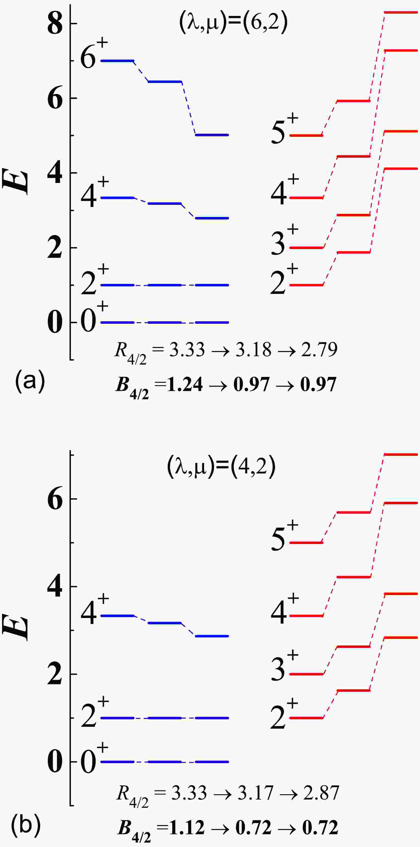
To illustrate band mixing in a two-band $S U^* $(3) system, the level patterns for $ (\lambda,\mu)=(6,2) $ and $ (\lambda,\mu)=(4,2) $, obtained from solving the Hamiltonian (5), are presented in Fig. 1. As observed in Fig. 1(a), significant changes in the normalized level energies occur as $ |\eta/\kappa| $ increases, which aligns with the analytical expressions given in (15)−(19). More importantly, the results demonstrate that the three-body term in the $S U^* $(3) limit can induce a $ B_{4/2}<1.0 $ feature while preserving the regularity of level pattern. In contrast to $ R_{4/2} $, it is evident that the $ B_{4/2} $ value remains independent of the absolute values of $ \eta/\kappa $ when $ \eta\neq0 $. This suggests that $ B_{4/2}<1.0 $ phenomenon caused by band mixing is an intrinsic characteristic of the $S U^* $(3) limit. This observation can be understood by noting that the wave functions for a given $ (\lambda,\mu) $ and L are primarily determined by the presence of the three-body term, as indicated by (10). Consequently, the strength parameter η acts as a scaling factor for all states within a given $ (\lambda,\mu) $, leaving the wave functions unchanged with respect to η.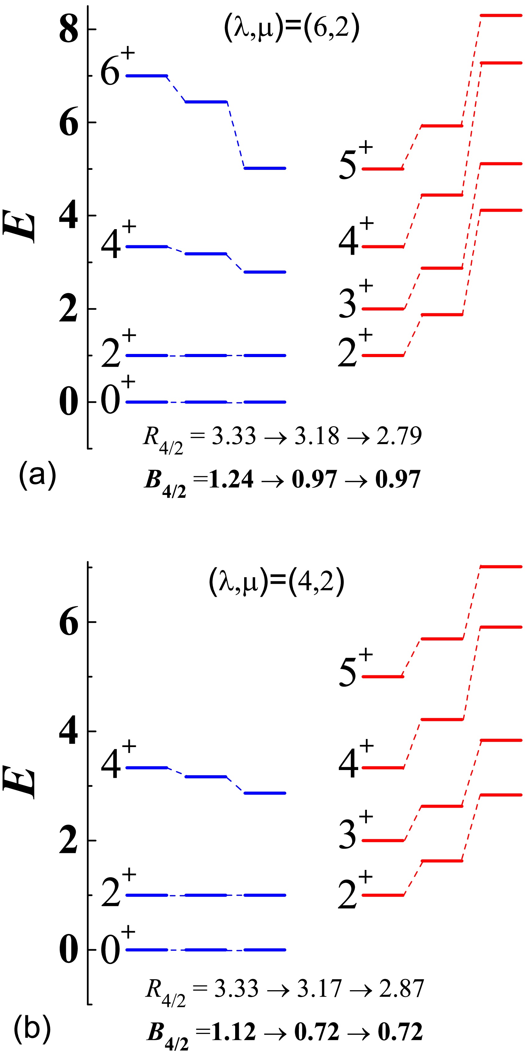

Figure 1.  (color online) (a) The low-lying level patterns for $ (\lambda,\mu)=(6,2) $, obtained for $ \eta/\kappa=0.0,-0.1,-0.2 $ (from left to right), are shown. (b) The same as in (a) but for $ (\lambda,\mu)=(4,2) $. In each panel, the level energies have been normalized to $ E(2_1^+)=1.0 $.

As indicated by the IBM-1 analysis [8, 10, 13], the anomalous $ E2 $ behavior of yrast states tends to in occur in systems characterized by intrinsic or dynamic triaxial deformation. In the $S U^* $(3) limit, γ deformations can be estimated from Eq. (11), yielding $ \gamma\simeq17^\circ $ for $ (\lambda,\mu)=(6,2) $. In addition to $ B_{4/2}=0.97 $, the $ (\lambda,\mu)=(6,2) $ configuration results in $ B(E2;6_1^+\rightarrow4_1^+)/B(E2;2_1^+\rightarrow0_1^+)=0.61 $ and $ B(E2;8_1^+\rightarrow6_1^+)/B(E2;2_1^+\rightarrow0_1^+)=0.0 $. From these results, two conclusions can be drawn: (a) $ B(E2) $ anomaly extends to yrast states with higher spins; (b) Transition $ B(E2;L_1^+\rightarrow (L-2)_1^+) $ for $ L>\lambda $ is forbidden due to the termination of the ground-state band at $ L={\rm{max}}[\lambda,\mu] $. These findings serve as signatures for a two-fluid system dominated by the $S U^* $(3) symmetry with the ground-state configuration $ (\lambda,\mu)=(2N_\pi,2N_\nu) $ or $ (2N_\nu,2N_\pi) $. As shown in Fig. 1(b), the two-band system for $ (\lambda,\mu)=(4,2) $ exhibits dynamic features similar to those of $ (\lambda,\mu)=(6,2) $. However, the $ B_{4/2} $ ratio for $ (\lambda,\mu)=(4,2) $, corresponding to $ \gamma\simeq22^\circ $, is notably lower than that for $ (\lambda,\mu)=(6,2) $, which corresponds to $ \gamma\simeq17^\circ $. This highlights the influence of triaxial deformation on the $ B(E2) $ structure.

The analysis for $ (\lambda,\mu)=(\lambda,2) $ can be directly extended to more general $S U $(3) IRREPs. Nevertheless, for cases with $ (\lambda,\mu>2) $, model solutions can only be obtained numerically. Due to the symmetric properties of the $S U $(3) Wigner coefficients under the transformation $ (\lambda,\mu)\rightarrow (\mu,\lambda) $ [39], the energies and $ B(E2) $ transitions derived from $ (\lambda,\mu)=(a,b) $ are identical to those from $ (\lambda,\mu)=(b,a) $ after changing the parameter η in (5) to $ -\eta $. This implies that $ \eta<0 $ must be used for cases where $ \lambda<\mu $ to ensure the regularity of yrast levels expected for a collective mode. In addition, it can be verified that interchanging λ and μ transforms the γ deformation from $ \gamma=A $ to $ \gamma=60^\circ-A $, as well as the quadrupole moment from $ \hat{Q}(2_1^+)=B $ to $ \hat{Q}(2_1^+)=-B $. To systematically analyze the $S U^* $(3) system, the γ deformation and $ B_{4/2} $ ratio obtained from different μ values are plotted as functions of λ in Fig. 2. As shown in Fig. 2(a), the γ values decrease monotonically with increasing λ within the range $ \gamma\in(0^\circ,60^\circ) $, reaching $ \gamma=30^\circ $ at $ \lambda=\mu $, which corresponds to maximal triaxial deformation. In contrast, Fig. 2(b) illustrates that the $ B_{4/2} $ ratio as a function of λ exhibits non-monotonic behavior, with minima occurring at $ \lambda=\mu $. Consequently, the lowest $ B_{4/2} $ ratios, potentially leading to $ B_{4/2}<1.0 $, favor maximal triaxialilty. It is important to note that the $ B_{4/2} $ results presented in Fig. 2(b) are independent of the absolute value $ |\eta/\kappa| $ for each given $ (\lambda,\mu) $, as confirmed by numerical calculations. Therefore, the observed $ B(E2) $ anomaly in the $S U^* $(3) limit is indeed an intrinsic feature resulting from band mixing.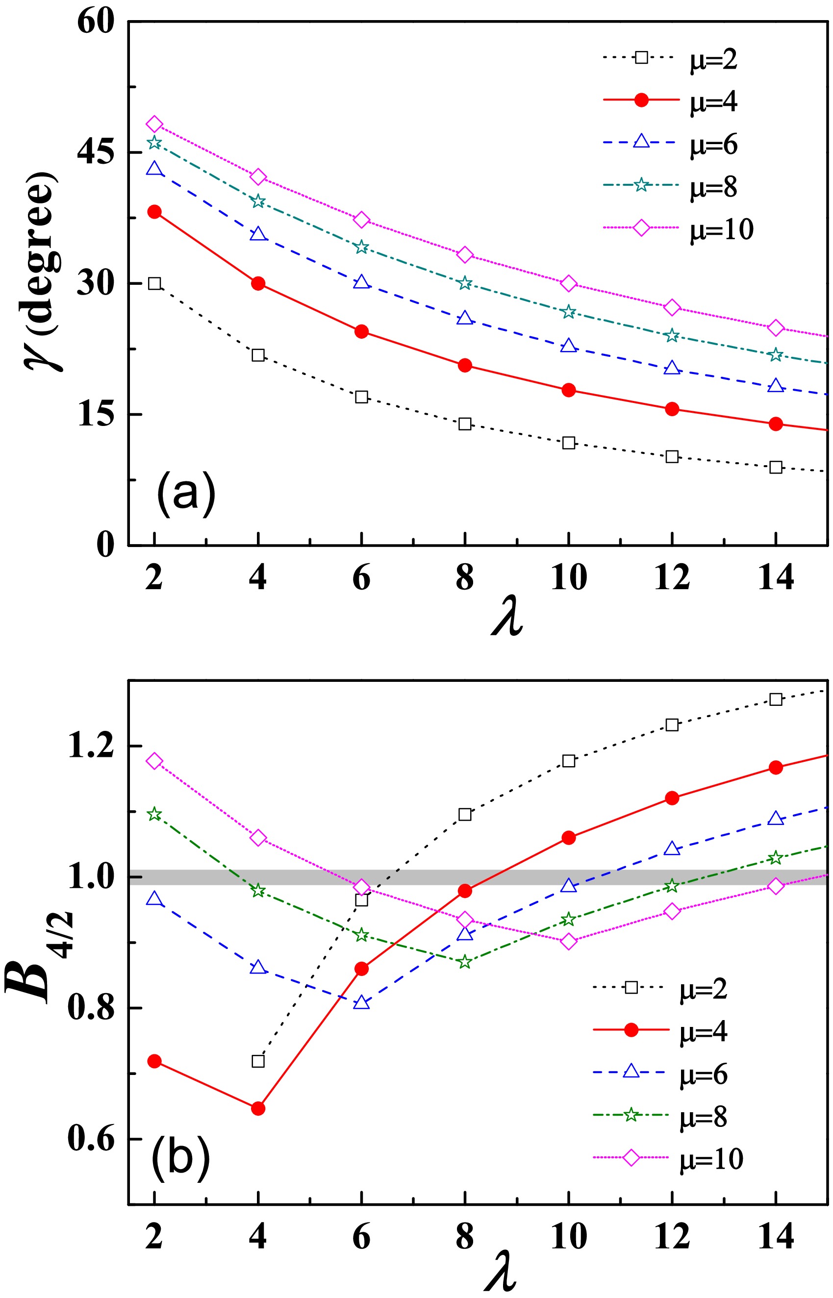

Figure 2.  (color online) (a) The γ deformations for different ($ \lambda,\mu $), calculated based on Eq. (11), are presented as a function of λ. (b) The corresponding $ B_{4/2} $ ratio for different ($ \lambda,\mu $) solved from the Hamiltonian (5) are shown as a function of λ. For $ \lambda\geq\mu $, the parameter in calculation is set to $ \eta/\kappa=-0.05 $, while for $ \lambda<\mu $, it is set to $ \eta/\kappa=0.05 $. In addition, $ B_{4/2} $ for $ (\lambda,\mu)=(2,2) $ is not shown because the ground-state band in this case terminates at $ 2_1^+ $.

To gain a deeper understanding of the $ B(E2) $ structure of yrast band, Fig. 3 presents the cascades defined as $ B_{L/2}\equiv B(E2;L_1^+\rightarrow (L-2)_1^+)/B(E2;2_1^+\rightarrow0_1^+) $, calculated under various symmetry limits with $ (N_\pi,N_\nu)=(4,5) $ and two cases breaking the ideal $S U^* $(3) dynamical symmetry. Additionally, experimental data for ¹⁰²Mo [40], ¹⁵⁰Ce [41] and ¹⁶⁶W [3], all characterized by $ (N_\pi,\; N_\nu)=(4,\; 5) $, are also included for comparative analysis. These experimental data are incorporated here to illustrate typical realistic scenarios rather than to achieve the best fit in theory. In the calculations, the Hamiltonian parameters are set as follows: $ (\chi_\pi,\; \chi_\nu,\; \eta/\kappa)=(-\sqrt{7}/2,\; -\sqrt{7}/2,\; -0.1) $ for the $S U $(3) limit, $ (\chi_\pi,\; \chi_\nu,\; \eta/\kappa)=(0,\; 0,\; -0.1) $ for the O(6) limit, and $ (\chi_\pi,\; \chi_\nu,\; \eta/\kappa)=(\sqrt{7}/2,\; -\sqrt{7}/2,\; -0.1) $ for the $S U^* $(3) limit. For scenarios deviating from the $S U^* $(3) limit, referred to as $S U^* $(3) breaking, we present two examples where $ \chi_\pi=\sqrt{7}/2 $ but $ \chi_\nu\neq-\sqrt{7}/2 $. Specifically, the parameter sets are chosen as $ (\chi_\pi,\; \chi_\nu,\; \eta/\kappa)=(\sqrt{7}/2,\; -0.7, -0.15) $ and $ (\sqrt{7}/2,\; -0.3,\; -0.26) $, respectively. The corresponding results, labeled as Cal.A and Cal.B, are illustrated in Fig. 3. To perform calculations in cases beyond the $S U $(3) symmetry limit, we have adopted the numerical scheme proposed in [42] for solving the IBM-2 Hamiltonian. As shown in Fig. 3, the ratio values in the $S U $(3) and O(6) limits consistently exhibit $ B_{L/2}\geq1.0 $, even when incorporating the three-body term as described in Eq. (5). Conversely, a monotonic decrease in the cascades as a function of L is observed in the $S U^* $(3) limit, which generates the ground-state IRREP $ (\lambda,\mu)=(10,8) $ for $ (N_\pi,\; N_\nu)=(4,\; 5) $. This indicates that the $ B(E2) $ anomaly in the $S U^* $(3) limit, characterized by $ B_{L/2}<1.0 $, persists throughout the entire yrast line, as exemplified by the $ (\lambda,\mu=2) $ cases discussed earlier. Furthermore, such anomalous features are accentuated in the $S U^* $(3) breaking scenarios, which appears to be supported by the available data for ¹⁵⁰Ce and ¹⁶⁶W. In contrast, the data for ¹⁰²Mo align more closely with the "normal" modes described by the $S U $(3) or O(6) limits. These findings, to some extent, provide evidences for the band-mixing induced $ B(E2) $ anomaly in the IBM-2 near the triaxial $S U^* $(3) limit.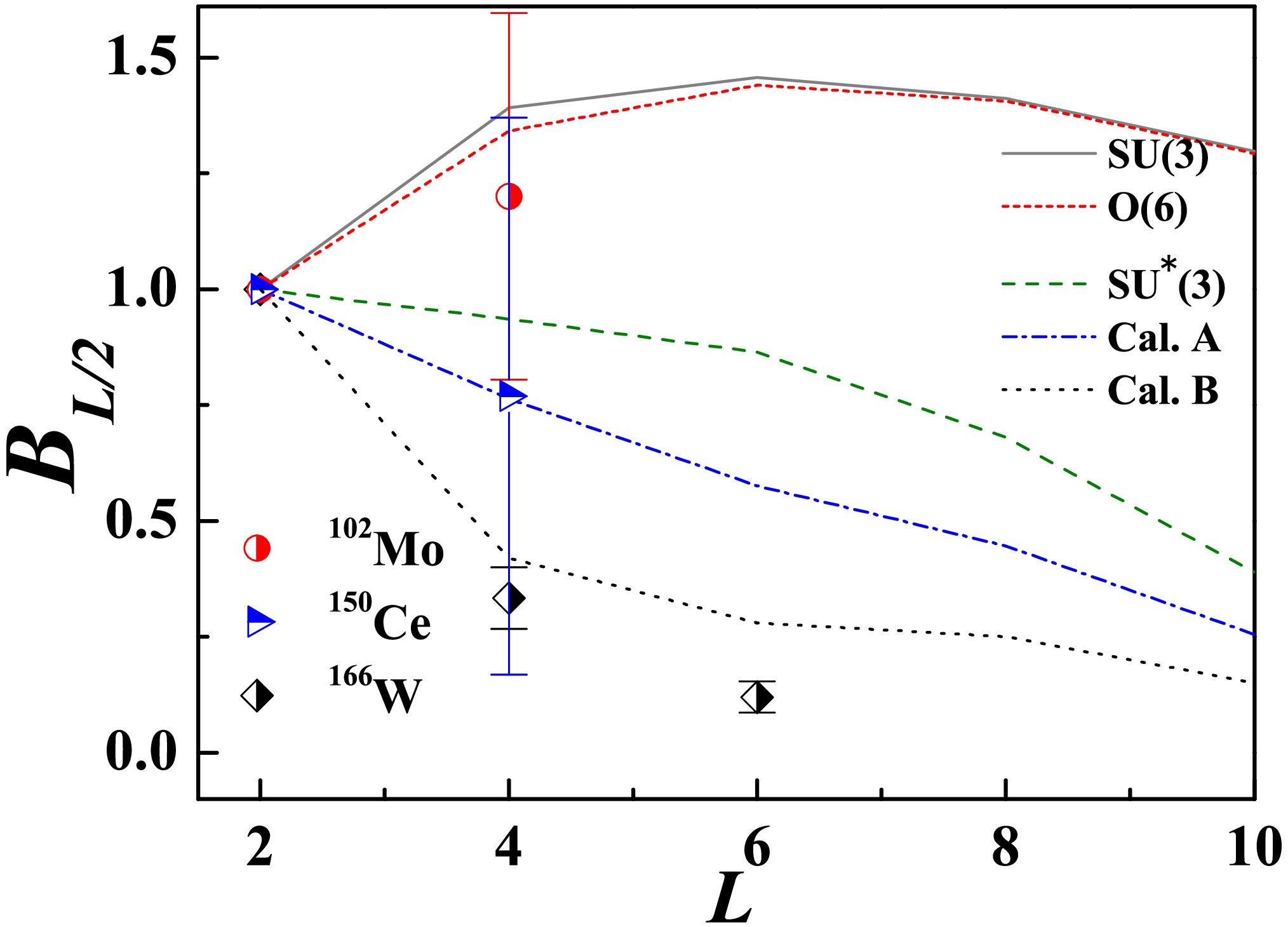

Figure 3.  (color online) The cascades of $ B_{L/2}\equiv B(E2;L_1^+\rightarrow $$ (L-2)_1^+)/B(E2;2_1^+\rightarrow0_1^+) $ obtained for the $S U $(3) limit, O(6) limit, $S U^* $(3) limi, as well as two examples (labeled as Cal.A and Cal.B) deviating from the $S U^* $(3) limit are presented (the parameters are detailed in the text). Experimental data [3, 40, 41] for nuclei corresponding to $ (N_\pi,\; N_\nu)=(4,\; 5) $ are included for comparative analysis.

Although the mean-field calculations suggest [33] that the ideal $S U^* $(3) system in the large-N limit comprise a proton fluid with oblate (prolate) deformation coupled to a neutron fluid with prolate (oblate) deformation [33], this does not imply that a realistic scenario with opposite sign of $ \chi_\pi $ and $ \chi_\nu $ is necessarily associated with completely inverse γ deformations between protons and neutrons. This point can be partially understood by examining the calculated quadrupole moments for proton and neutron bosons via $ \hat{Q}_\rho(L^+)=\sqrt{\dfrac{16\pi}{5}}\langle LM|\hat{Q}_\rho|LM\rangle_{M=L} $. For instance, adopting the same parameters as those used in Fig. 3, it is shown both $ \hat{Q}_\pi(2_1^+)<0 $ and $ \hat{Q}_\nu(2_1^+)<0 $ for the case of Cal.A, while both $ \hat{Q}_\pi(2_1^+)>0 $ and $ \hat{Q}_\nu(2_1^+)>0 $ for the case of Cal. B. This suggests that the γ deformations of low-spin states are influenced not only by the $ \chi_{\pi(\nu)} $ values but also by the boson numbers $ N_{\pi(\nu)} $ and the strength ratio $ \eta/\kappa $, when using the simple Hamiltonian form (5). Additionally, the results indicate that relatively large fluctuations in γ are anticipated for the $ B(E2) $ anomaly systems when deviating from the ideal $S U^* $(3) limit. This observation aligns with the recent analysis of $ B(E2) $ anomaly within the IBM-1 framework presented in [13]. That study demonstrates that the $ B(E2) $ anomaly features arising from band mixing can be modeled even using a Hamiltonian with zero γ deformation at the mean-field level, yet exhibiting pronounced γ softness. As a result, a meaningful evaluation of the current theoretical perspective involves finding a method to determine the effective γ deformation [43] or γ fluctuations in $ B(E2) $ anomaly systems. Further discussions on γ fluctuations within the IBM-2 framework will be addressed elsewhere.

In summary, a theoretical analysis of the potential correlation between the $ B(E2) $ anomaly phenomenon and triaxial deformation has been conducted within the framework of the IBM-2. The results demonstrate that the anomalous $ E2 $ behaviors, characterized by $ B_{4/2}<1.0 $, can naturally arise from the $S U^* $(3) dynamical symmetry limit of the IBM-2 when a three-body term is incorporated alongside the quadrupole-quadrupole interaction. This offers a clear symmetry-based interpretation of the $ B(E2) $ anomaly features arising from band mixing, which were identified in the IBM-1 but described through complex polynomial combinations of various high-order terms [8–13]. Beyond the analytic explanation based on the ideal $S U^* $(3) limit, which models a triaxially deformed two-fluid system, it is shown that the $S U^* $(3) breaking effects are crucial for providing a qualitative description of the experimentally observed $ B(E2) $ anomaly. This conclusion is supported by available experimental data for relevant nuclei. In addition to even-even systems, similar observations of the $ B(E2) $ anomaly phenomenon have also been reported in odd-A species [6]. Extending this symmetry-based analysis to odd-A systems [12] and to other $S U $(3)-related microscopic framework [44, 45] would be interesting. Related work is in progress.