Harvesting entanglement from cylindrical gravitational wave spacetime

Entanglement harvesting [1, 2] refers to the process by which detectors independently coupled to a quantum field can become entangled by extracting entanglement from the field. This mechanism operates within a multipartite quantum system framework, comprising the combined Hilbert spaces of the detectors and field. Typically modeled using a scalar field, this setup facilitates the transfer of virtual particles between detectors, thereby inducing entanglement among them. The possibility of entanglement harvesting from spacelike separated regions is unique to quantum fields, as classical fields do not possess entanglement that can be extracted. This distinction has been utilized to determine the quantum or classical nature of a field. Notably, it has been proposed that employing an entanglement harvesting protocol with the gravitational field could serve as a direct witness to quantum gravity [3, 4]. This approach underscores the pivotal role of quantum field properties in facilitating such quantum phenomena.

Initially explored in flat spacetime scenarios [1, 2], the phenomenon of entanglement harvesting has been extensively investigated under various conditions, including cosmological backgrounds [5, 6], noninertial frames [7, 8], and black hole environments [9, 10], and in the presence of gravitational waves (GWs) [11, 12]. Further studies have considered entanglement harvesting when detectors interact with distinct field operators [13−15] and when placed in superpositions of different temporal orders or trajectories [16, 17].

The entanglement harvested by two Unruh-DeWitt (UDW) detectors [18, 19] is highly sensitive to the frequency of the gravitational wave. This can reveal the "information content" about gravitational-wave memory effect and supertranslations [11, 12]. Other investigations into entanglement harvesting from the vacuum including gravitational waves involved the quantum degrees of freedom of gravity by coupling GWs to a scalar quantum field [20−22]. In these studies, the GWs were considered as planar waves, which can manifest that the vacuum in the presence of GWs are quantum but cannot reveal any other information about the wave sources. In this paper, we investigate entanglement harvesting in the context of cylindrical GWs of Einstein and Rosen (also called Einstein-Rosen waves, or ERWs) [23−26] and discuss the distance from the wave sources obtained through analyses of the entanglement change between two UDW detectors.

The ERW, an exact solution to general relativity characterized by two commuting Killing vectors, aptly describes a cylindrical GW. Historically, the ERW was pivotal in early explorations to quantify the energy transported by GWs [28−31], a challenging task owing to the local nondescriptiveness of GW energy caused by the equivalence principle [32, 33], which showed that the observation of ERWs is feasible. Moreover, the quantum aspects of ERWs have been rigorously formulated [34], and their quantization in conjunction with a massless scalar field has been successfully achieved [35]. This facilitates the study of entanglement harvesting from the perspective of ERW spacetime. In particular, ERWs carry information about the distance from the wave sources, which might be transferred to the harvested entanglement between the detectors, as will be investigated in this paper.

This paper is organized as follows. In Section II, the protocol of entanglement harvesting is revisited using two spacelike separated detectors that are accelerating in the flat spacetime. In Section III, the quantized formalism of the weak cylindrical GWs, and how the detectors are coupled to the GWs are described. Meanwhile, entanglement harvesting from the spacetime in the presence of linear cylindrical GWs is studied and the information about the distance from the wave sources is revealed in this section. The conclusions is given in Section IV.

We consider two identical UDW detectors, labeled A and B. Each detector is a two-level system with ground state $ \left\vert g\right\rangle _{D} $ and excited state $ \left\vert e\right\rangle _{D} $, where $ D\in\{{A,B\}} $. The energy difference between these states is denoted by $ \Omega_{D} $. These detectors interact locally with a massless quantum scalar field, represented by $ \hat{\phi}(x,t) $. The path followed by each detector through spacetime is specified by $ x_{D}(\tau_{D}) $, where $ \tau_{D} $ is the proper time experienced by detector D. The interaction between each detector and the scalar field is governed by a Hamiltonian specific to each detector:

where $ \lambda_{D}\ll1 $ represents a small coupling strength of each detector to the scalar field. The switching function $ \chi_{D}(\tau) $ regulates the timing of the interaction, turning the coupling to the field on and off. $ f_{D}(x) $ is the smearing function which controls the spatial region of the interaction. The ladder operators, which facilitate transitions between the detector states, are defined as $ \sigma_{D}^{+} = \left\vert e\right\rangle _{D}\left\langle g\right\vert _{D} $ and $\sigma_{D}^{-} = \left\vert g\right\rangle _{D}\left\langle e\right\vert _{D}$. These operators are crucial in our quantum mechanical model, which effectively describes light-matter interactions without involving angular momentum exchange.

The time evolution of the detector-field system is governed by the unitary operator $ \hat{U} $, defined as

where $ {\cal{T}} $ is the time-ordering operator that arranges the operators from earliest to latest times as we move from right to left in the exponential.

Initially, both detectors A and B start in their ground states, and the field is in its vacuum state. The combined initial state of the system is

After the interaction, the state of the detectors is described by density matrix $ \hat{\rho}_{AB} = Tr_{\phi}\left[ \hat{U}\left\vert \varphi _{0}\right\rangle \left\langle \varphi_{0}\right\vert \hat{U}^{\dagger }\right] $, obtained by tracing the field states from the total system state. This results in

to the lowest order in coupling strength. The density matrix (4) is expressed by basis $ \{\left\vert g_{A}g_{B}\right\rangle ,\left\vert g_{A}e_{B}\right\rangle ,\left\vert e_{A}g_{B}\right\rangle , \left\vert e_{A}e_{B}\right\rangle \} $. Here, $ {\cal{L}}_{AA} $ and $ {\cal{L}}_{BB} $ represent the probabilities of detectors being excited, and $ {\cal{L}}_{AB} $, $ {\cal{L}}_{BA} $, and $ {\cal{M}} $ measure the coherence between the detectors due to their interaction with the field, reflecting nonlocal effects between the two detectors at different times.

and

where $ \theta(t-t^{\prime}) $ is the Heaviside function. Wightman function $ W(x,x^{\prime}) = \langle0|\hat{\phi}\left( x(t),t\right) ,\hat{\phi}\left( x^{\prime}(t^{\prime}),t^{\prime}\right) |0\rangle $ is a fundamental field correlator that quantifies the vacuum fluctuations of the field between two spacetime points $ x(t) $ and $ x^{\prime}(t^{\prime}) $, making it crucial for understanding the field's influence on detectors.

When we consider only one of the detectors, either A or B, by tracing the other one from the combined density matrix (Eq. 4), we arrive at a simplified description for the state of the remaining detector:

In this matrix, $ {\cal{L}}_{C} $ represents the probability that detector A or B transitions from its ground state to its excited state owing to its interaction with the field.

To explore the entanglement between two identical UDW detectors after local interactions with a quantum field, we use a measure called negativity [36, 37]. Negativity is a reliable quantifier for entanglement between two qubits, suitable for situations such as entanglement harvesting, as discussed in previous studies. The negativity of a system, $ {\cal{N}} $, is determined by summing the negative eigenvalues from the partial transpose of density matrix $ \hat{\rho}_{D} $:

In cases where the detectors have equal excitation probabilities, $ {\cal{L}}_{AA} = {\cal{L}}_{BB} = {\cal{L}} $, the formula simplifies to

Assuming both detectors are identical with equal interaction strengths, frequencies, and simultaneous interactions in their respective frames, we can use the following expressions to compute the necessary probabilities and correlation terms from the Fourier transforms of the switching functions:

where

and we define the Fourier transforms of $ f({\bf{x}}) = \psi _{e}({\bf{x}})\psi_{g}^{\ast}({\bf{x}}) $ and $ \chi(t) $ as

Note that the results are obtained using the assumption that $ \lambda_{A} = \lambda_{B} = \lambda $, $ \Omega_{A} = \Omega_{B} = \Omega $, $ \chi _{A}(t) = \chi_{B}(t) = \chi(t) $, and the smearings are identical modulo a spatial translation. Hereinafter, this assumption will be maintained.

The concept of entanglement harvesting using two UDW detectors linearly coupled to a scalar quantum field has been investigated in the literature [8, 9, 11, 14, 17, 38−41]. However, in curved spacetime, what information about the curved spacetime can be obtained from the harvested entanglement has barely been investigated. This is the aim of this paper, and in the following, we investigate how to extract information about the distance from the wave sources by the harvested entanglement from the vacuum of cylindrical GW spacetime.

In this section, we study the situation in which two UDW detectors are coupled to cylindrical GWs. We implement the entanglement harvesting protocol and analyze the information about the distance from the wave sources using Fisher information.

Because the observable effect of cylindrical GWs is considered at a large distance from the source, the following linearized metric is adequate for our purposes:

where $ {\rm d}s_{3}^{2} = -\left( 1+\gamma\right) {\rm d}T_{C}^{2}+\left( 1+\gamma \right) {\rm d}R^{2}+R^{2}{\rm d} \theta^{2} $, and ψ and γ are the functions of only R and $ T_{C} $. This is derived from the spacetime metric of ERWs [23, 34, 42, 43], ${\rm d}s^{2} = {\rm e}^{\gamma-\psi}(-{\rm d}T_{C}^{2} + {\rm d}R^{2})+ {\rm e}^{-\psi}R^{2}{\rm d}\theta^{2}+{\rm e}^{\psi}{\rm d}Z^{2}$, where ψ encodes the physical degrees of freedom and satisfies the usual wave equation for an axially symmetric massless scalar field in three-dimensions,

Metric function γ can be expressed as [44] $ \gamma (R) = \dfrac{1}{2}\displaystyle\int_{0}^{R}\mathrm{d}\bar{R}\,\bar{R}\,\left[ (\partial_{T_{C}} \psi)^{2}+(\partial_{\bar{R}}\psi)^{2}\right] $ and $\gamma_{\infty} = \dfrac {1}{2}\displaystyle\int_{0}^{\infty}\mathrm{d}R\,R\, \left[ (\partial_{T_{C}}\psi)^{2}+(\partial _{R}\psi)^{2}\right]$, where $ \gamma(R) $ and $ \gamma_{\infty} $ are the energy of the scalar field in a ball of radius R and in the whole two-dimensional flat space, respectively.

When regularity at origin $ R = 0 $ is imposed [44], the solutions for the field ψ can be expanded in the form

where $A({\boldsymbol{k}})$ and $A^{\dagger}({\boldsymbol{k}})$ are fixed by the initial conditions and are complex conjugates to each other, as ψ and $ J_{0} $ (the zeroth-order Bessel function of the first kind) are real. In principle, the quantization of field ψ can be carried out in a standard way. We can introduce a Fock space in which $ \hat{\psi}(R,0) $, the quantum counterpart of $ \psi(R,0) $, is an operator-valued distribution [45]. Its action is determined by the usual annihilation and creation operators, $\hat {A}({\boldsymbol{k}})$ and $\hat{A}^{\dagger}({\boldsymbol{k}})$, respectively, whose only nonvanishing commutators are$\left[ \hat{A}({\boldsymbol{k}}_{1}),\hat{A}^{\dagger} ({\boldsymbol{k}}_{2})\right] = \delta({\boldsymbol{k}}_{1},{\boldsymbol{k}}_{2}).$

The Hamiltonian of this linearized gravity can be written as [34, 42, 46]

where gauge fixing conditions $ p_{\gamma} = 0 $ and $ R = r $. $ p_{\hat{\psi}} $ and $ p_{\gamma} $ are the canonical momenta conjugated to metric fields $ \hat{\psi} $ and γ, respectively. $ R = r $ indicates that R can be used to measure the distance from the source to detector. It is straightforward to confirm that $H_{0} = \gamma_{\infty} =$ $\displaystyle\int_{0}^{\infty}\mathrm{d}{\boldsymbol{k}} \,{\boldsymbol{k}}\hat{A}^{\dagger}({\boldsymbol{k}})\hat{A}({\boldsymbol{k}})$ when the expression of $ p_{\hat{\psi}} $ is used.

To obtain a unit asymptotic timelike Killing vector field in the actual four-dimensional spacetime [47, 48], one must transfer the time coordinate by $T_{C} = \mathrm{e}^{-\gamma_{\infty}/2}t$. In this asymptotic region, $ R\rightarrow\infty $, $ \partial_{t} $ is a unit timelike vector, t is the physical time, and the corresponding physical Hamiltonian is given as [42, 47, 48] $H = E(H_{0}) = 2(1-\mathrm{e}^{-H_{0}/2})$. Thus, the annihilation operator with respect to physical time can be linked to $\hat {A}({\boldsymbol{k}})$ by $\hat{A}_{E}({\boldsymbol{k}},t) = \hat{A}({\boldsymbol{k}} )\exp[-\mathrm{i}tE({\boldsymbol{k}}) {\rm e}^{-H_{0}/2}]$. In the first approximation, the physical field $\hat{\psi} = \displaystyle\int_{0}^{\infty}\dfrac{\mathrm{d}{\boldsymbol{k}}}{\sqrt{2}} \,J_{0}(R{\boldsymbol{k}})\big[ \hat{A}_{E}({\boldsymbol{k}},t)+\hat{A}_{E}^{\dagger }({\boldsymbol{k}},t)\big]$ has a similar time-evolved form to Eq. (17). When the UDW detectors are coupled to the linearized cylindrical GWs, physical Hamiltonian H should be considered, but in the first-order perturbation,$ H\simeq H_{0} $ and $ t\simeq T_{C} $. Thus, the results in the coordinates ($T_{C}, R, \theta, Z$) can be used in the actual interaction between the detectors and linearized cylindrical GWs, as demonstrated in the next section.

We start with the interaction Hamiltonian between GWs and two free-falling detectors [15]

where $ \lambda = \sqrt{\dfrac{\pi}{2}}\dfrac{m}{m_{p}} $, with $ m_{p} $ being the Planck mass. Here, λ serves as a dimensionless coupling constant, essentially scaling with the detector's rest mass measured in Planck units. This formulation allows us to quantitatively assess the gravitational effects on quantum mechanical scales. There are some other ways (see the discussions in Ref. [15]) to describe the interaction between the detectors and an external weak gravitational field, while we choose the same way as in Ref. [15] which considers a wave function in curved spacetimes, because for our study, the quantum states for the detectors and quantum description for ERWs are explicit, as presented in the following calculations.

Assuming that the energy levels of our detector's free Hamiltonian are discrete, we can expand the interaction Hamiltonian in terms of the system's wavefunctions as

where $f_{nm}({\boldsymbol{x}}) = \psi_{n}({\boldsymbol{x}})\psi_{m}^{\ast}({\boldsymbol{x}})$ is the smearing function, $\left\vert {\boldsymbol{x}}\right\rangle \left\langle {\boldsymbol{x}}\right\vert _{t}$ denotes the position operator in the interaction picture, and the switching function is added here to ensure finite interaction time. Functions $\psi_{n}({\boldsymbol{x}}) = \left\langle {\boldsymbol{x}}|n\right\rangle$ represent the wavefunctions corresponding to the energy eigenvalues $ E_{n} $, and $ \Omega_{nm} = E_{n}-E_{m} $ represents the energy difference between states. In our calculation, the detectors are regarded as two-level atoms, such as the ground state and an excited state, and the corresponding wavefunctions are $\psi_{g}({\boldsymbol{x}}) = \left\langle {\boldsymbol{x}}|g\right\rangle$ for the ground state and $\psi_{e}({\boldsymbol{x}} ) = \left\langle {\boldsymbol{x}}|e\right\rangle$ for the excited state. This simplified model allows us to focus on the key dynamical aspects of the quantum system under the influence of an external gravitational field. Then, the interaction Hamiltonian can be written as

where the energy difference between excited state $ \left\vert e\right\rangle $ and ground state $ \left\vert g\right\rangle $ is denoted by $ \Omega = \Omega_{eg} = E_{e}-E_{g} $. Function $F^{ij}({\boldsymbol{x}}) = \psi _{e}({\boldsymbol{x}})\psi_{g}^{\ast}({\boldsymbol{x}})x^{i}x^{j}$ represents the smearing tensors, which are crucial for modeling the interaction of the detector with the linearized gravitational field. The ladder operators are defined as $ \hat{\sigma}^{+} = \left\vert e\right\rangle \left\langle g\right\vert $ and $ \hat{\sigma}^{-} = \left\vert g\right\rangle \left\langle e\right\vert $. Additionally, the terms in the Hamiltonian that commute with the detector's free Hamiltonian have been neglected, as they do not contribute to the entanglement dynamics but only shift the energy levels. Quantization can be implemented by replacing curvature tensor ${\cal{R}} _{0i0j}(t,{\boldsymbol{x}})$ with operator-valued distribution $ \hat {{\cal{R}}}_{0i0j}(x) $ in the Hamiltonian. This model provides a framework for understanding the interaction between a localized quantum system and weak quantum gravitational field.

To leading order in λ, the excitation probability of the detector after the interaction can be expressed as

This equation shows how the excitation probability can be transformed into a single momentum integral based on the curvature two-point function. This formulation is crucial for quantitatively describing how quantum systems respond to gravitational fields, offering insights into their probabilistic behavior under such influences. The curvature fluctuation, which is given by $ R_{0R0R}(R,T) = -\dfrac{1}{2}\partial_{T}^{2}h_{RR} $ ($ h_{RR} = \psi\left( R,T\right) $ as shown in Eq. (15)), can be obtained as

where Eq. (17) is used. Then, the curvature two-point function is calculated as

Thus,

where in the calculation, the switching functions are taken as $ \chi _{A}(t) = \chi_{B}(t) = $ $ \chi(t) = \dfrac{1}{\sqrt{2\pi}}\exp(-t^{2}/2T^{2}) $, and the smearing functions are taken as $ f_A(x)=\dfrac{1}{(2\pi\sigma^2)^{3/2}}\exp(-x^2/2\sigma^2), $$ f_{B}(x) = \dfrac{1}{(2\pi\sigma^{2})^{3/2} }\exp(-(x-L)^{2}/2\sigma^{2}) $, where T represents a duration timescale, σ determines the spatial width of the smearing function, and L is the separation between the detectors.

Similarly, given the choices of gaps and spacetime smearing functions, the resulting expression for nonlocal term $ {\cal{M}}^{G} $ can be obtained as

In Figs. 1, 2, and 3, we present the numerical results for negativity.

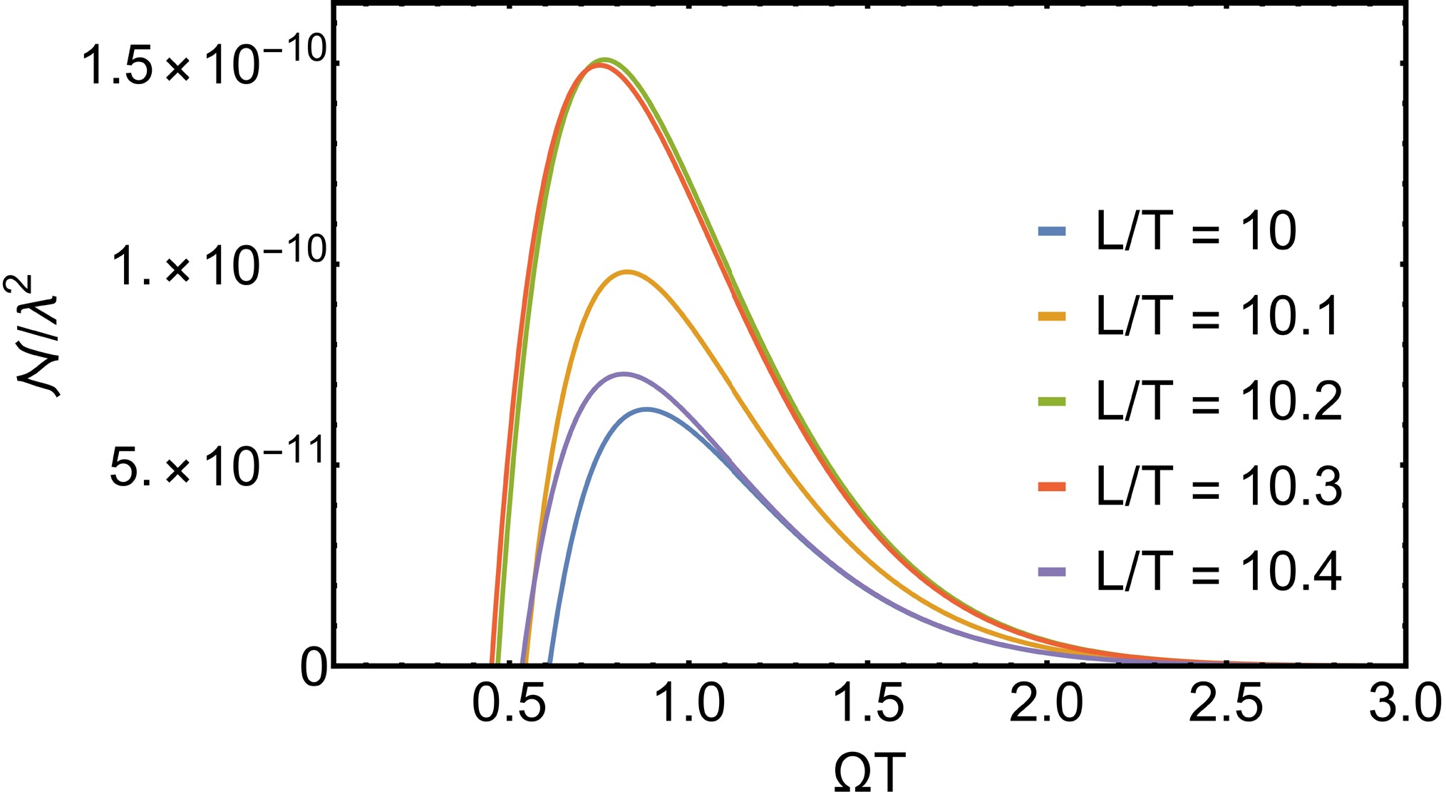
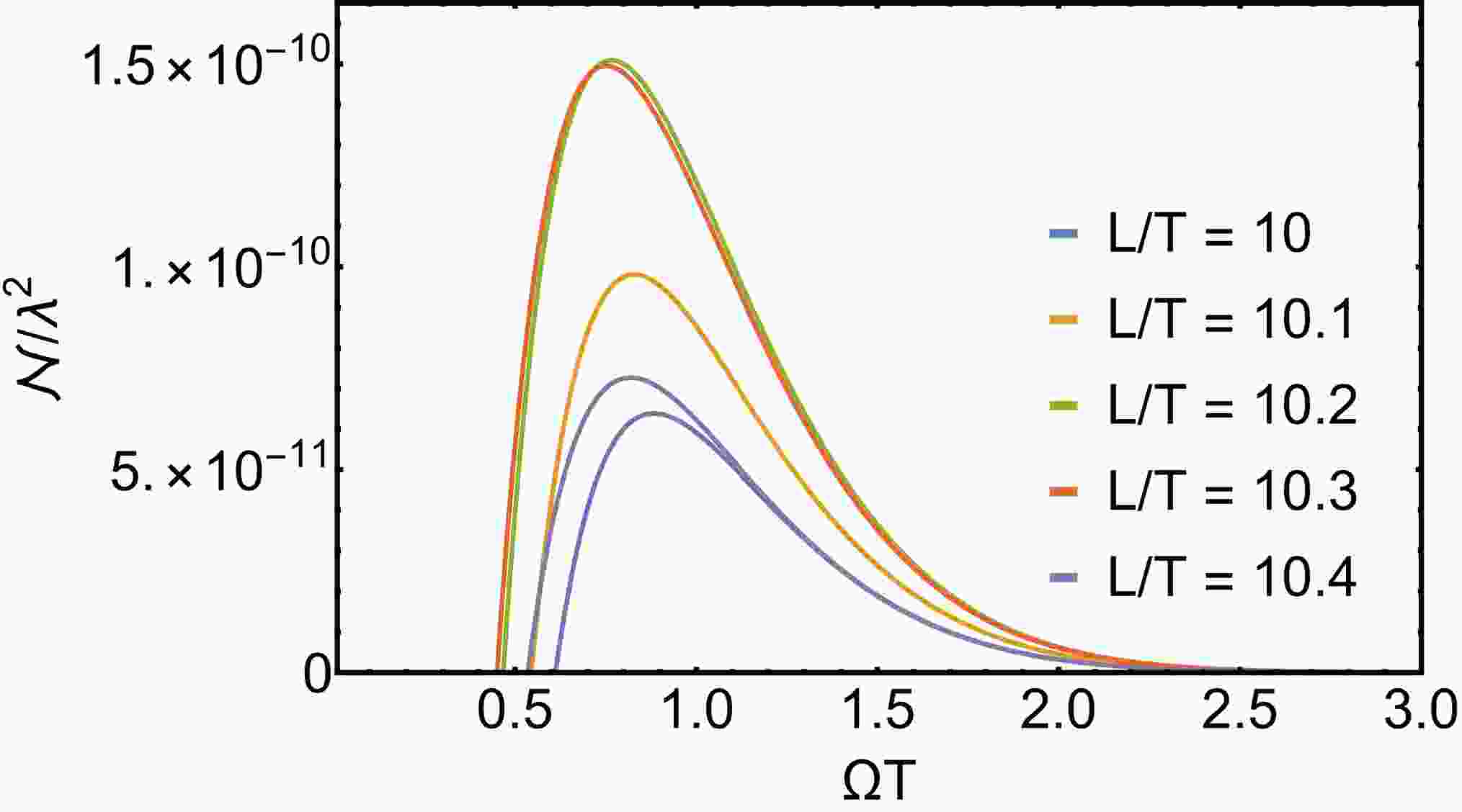
Figure 1.  (color online) Negativity as a function of the detectors' gap Ω for multiple values of detector separation distance L. We fixed the detector size to $ \sigma = 0.3T $ for each of the plots. Other parameter is taken as $ R/T = 1000 $.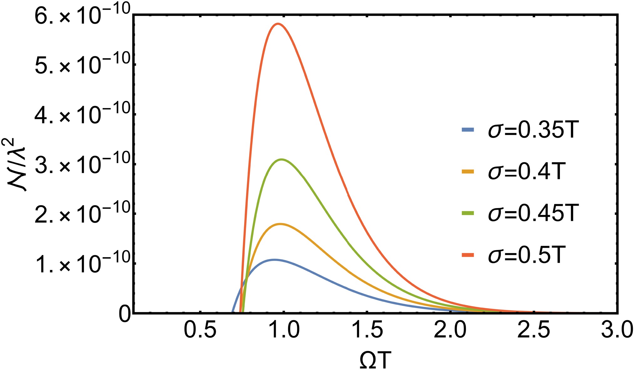

Figure 2.  (color online) Negativity as a function of the detectors' gap Ω for multiple values of detector size σ. We fixed the separation between the detectors to be $ L = 10 T $ for each of the plots. Other parameters is taken as $ R/T = 1000 $.

Figure 3.  (color online) Negativity as a function of detectors size σ for multiple values of detector separation L. We fixed the energy gap of the detectors as $ \Omega T = 0.77 $ for each of the plots. Other parameter is taken as $ R/T = 1000 $.

In Fig. 1, we plot the negativity of the two-detector system as a function of the detectors' energy gap for different values of the separation between them. We see that there is a minimum threshold on the required energy gap before any entanglement is acquired between the detectors. Once the threshold energy gap is met, there is a rapid increase in the negativity until it peaks. This is a similar behavior to entanglement harvesting from a real scalar field, where the detectors gap can be tuned to maximize the harvested entanglement (see [41]).

In Fig 2, we plot the entanglement acquired by the detectors as a function of their energy gaps for varying detector sizes. We conclude that as the detectors increase in size, the harvested entanglement increases. This can be traced back to the fact that the interaction of the detectors with the gravitational field is proportional to their sizes squared.

In Fig. 3, we plot the negativity of the detector state as a function of σ for a fixed $ \Omega T $ and varying values of L. We can clearly see a monotonic increase in the negativity with σ. We also see that the negativity decreases only after the ratio $ \sigma/T $ exceeds approximately $ 0.57 $ as the separation between the detectors increases.

In Fig. 4, we present how the entanglement harvested by detectors varies with the distance from the source of GWs, taking into account different distances between the detectors themselves. We find that the harvested entanglement diminishes as the source distance increases, a phenomenon linked to the weakening strength of GWs as they propagate from their origin.

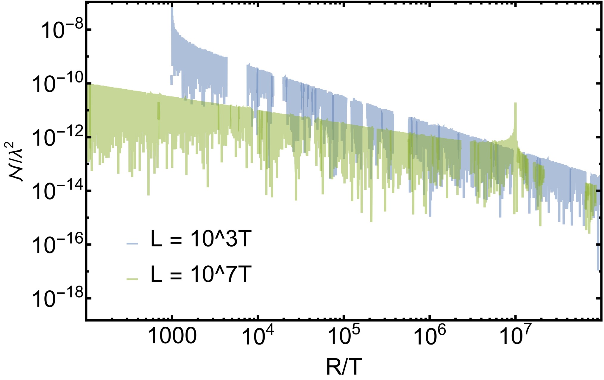
Figure 4.  (color online) Negativity as a function of GW source distance R for multiple values of detectors separation L. We fixed the energy gap of the detectors as $ \Omega T = 0.77 $ for each of the plots. Other parameters is taken as $ \sigma/T = 1000 $.

Additionally, in Fig. 5, we explore the relationship between the entanglement harvested by the detectors and their energy gap across various source distances. The analysis confirms that as the distance from the source increases, the entanglement decreases, underscoring the impact of GW attenuation over distance.

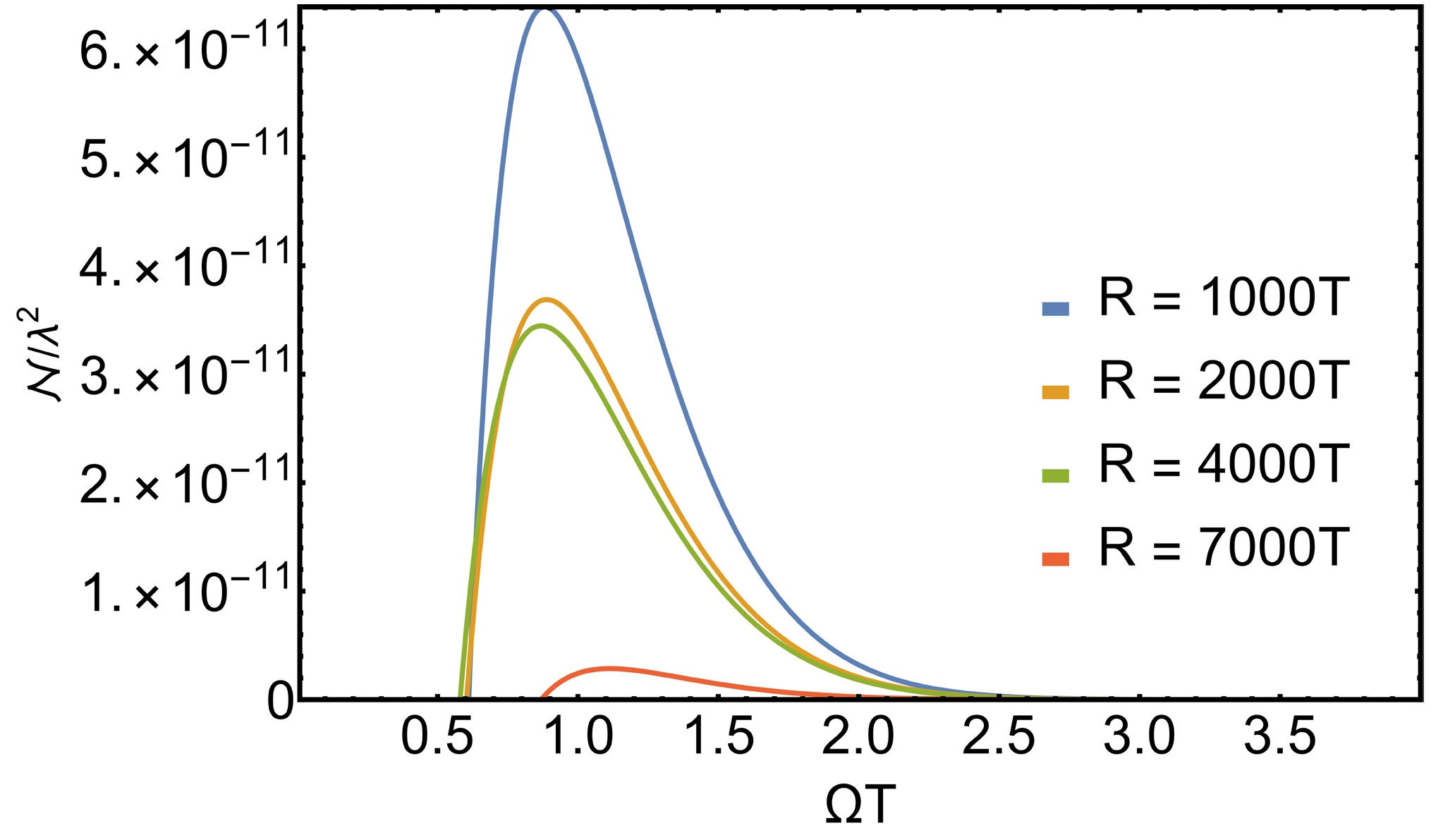
Figure 5.  (color online) Negativity as a function of energy gap for multiple values of source distance R. We fixed the detector separation as $ L = 10T $ for each of the plots. $ \sigma/T = 1000 $.

Finally, we comment on realistic scales for the entanglement that can be harvested by a physical system interacting with the cylindrical gravitational field. Our plots for the negativity yielded (at best) ${\cal{N}}^{G} \sim\lambda^{2}5\times10^{-7}$. Recall that dimensionless coupling constant λ is given by $ \sqrt{\dfrac{\pi}{2}}m/m_{p} $. If the mass of the system is of the order of the mass of a hydrogen atom we would have $ \lambda^{2} \sim10^{-38} $, so the harvested negativity gives $ {\cal{N}}^{G} \sim10^{-46} $. This result demonstrates that the entanglement harvested using cylindrical symmetry is significantly greater than that observed in entanglement harvesting from the gravitational field using hydrogen-like atoms at a source distance of $ R = 1000T $, as reported in [15]. Furthermore, even at a much larger distance of $ R = 9\times10^{7}T $, the harvested entanglement, $ {\cal{N}}^{G}\approx10^{-55} $, still exceeds previous findings by 16 orders of magnitude. These findings show the enhanced capability of detectors with cylindrical symmetry to harvest entanglement from the GW field.

To understand the distance from the sources, based on the cylindrical GWs, we apply the concept of quantum Fisher information (QFI) to investigate the possibility of measurement.

According to the quantum Cramér-Rao theorem [49, 50], for a given observable source distance R, the measurement precision is determined by

where $\mathrm{Var}$ is the covariant variance, and n represents the number of repeated measurements. $ {\cal{F}}_{Q} $ is the QFI defined by [51]

then we have the transition rate as

and

Finally, we obtain an expression for the QFI as

The measurement uncertainty is defined by

where $\sigma_{R} = \sqrt{\mathrm{Var}(R)}$. We found that, for our model, when the wave source distance satisfies $ R/L<200 $, the uncertainty in measuring the wave source distance is approximately 21%. Moreover, the QFI decreases rapidly as R increases, as shown in Fig. 6. This level of uncertainty is comparable to LIGO's measurements of binary neutron star merger events (10%−20%) and is lower than the uncertainty in measurements of binary black hole merger events (20%−50%) [52, 53]. Moreover, it is noted that Fig. 6 exhibits abrupt, nonsmooth behavior, which is derived from the oscillatory Bessel functions. These functions, combined with the exponential suppression term, introduce a resonance effect that leads to abrupt changes in the QFI.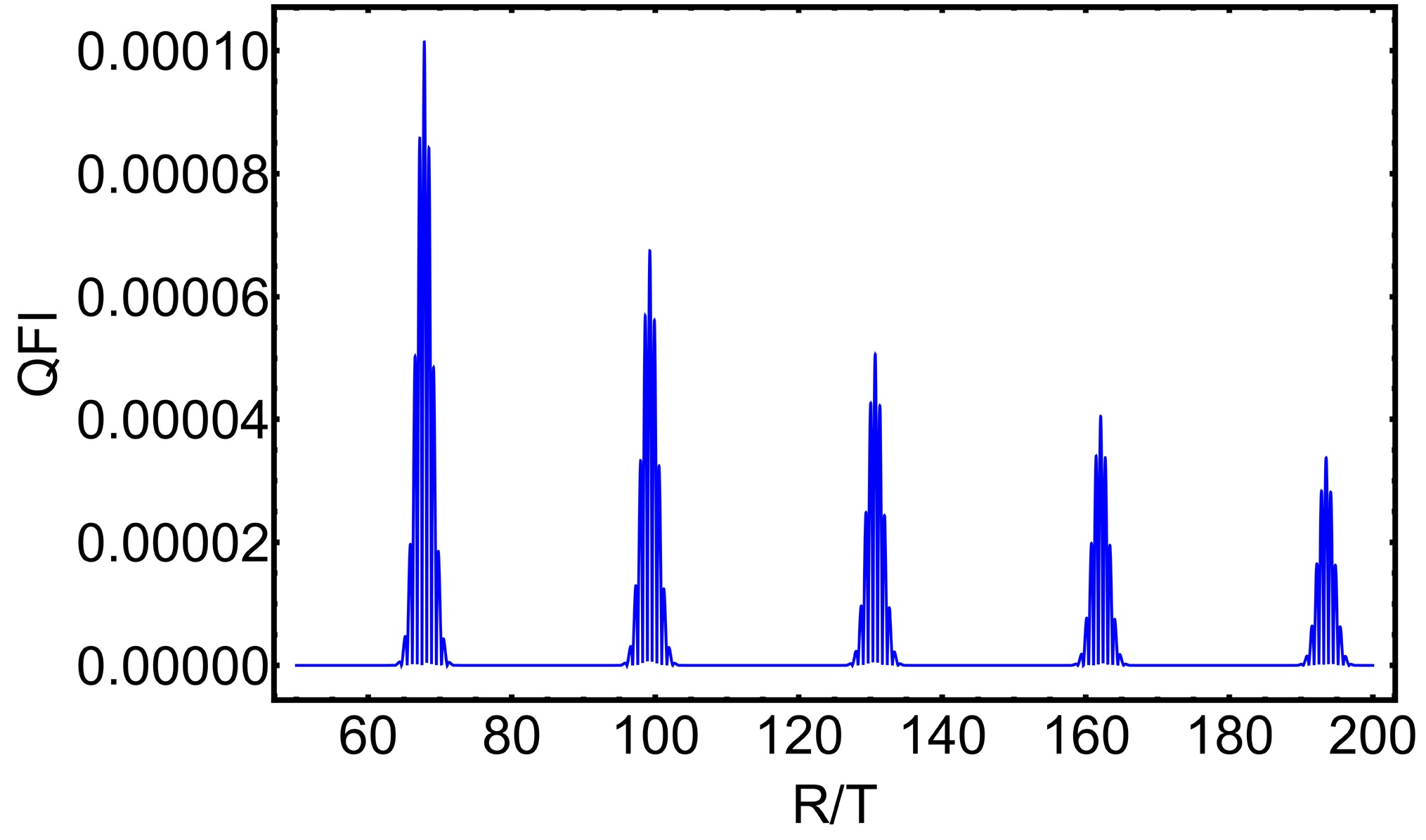

Figure 6.  (color online) Absolute value of QFI as a function of the normalized wave source distance. The parameters are $ \sigma = 0.3T $, $ \Omega T = 0.1 $, and $ L = 10T $.

In this study, we explored the entanglement harvesting protocol within spacetime in the presence of cylindrical GWs, revealing results that markedly contrast with those from scenarios involving standard quantum gravitational fields. The magnitude of entanglement negativity is substantially greater than that harvested from the vacuum of a conventional gravitational field. Importantly, our research elucidates the relationship between entanglement harvesting and the source distance of GWs.

This significant discrepancy highlights the unique quantum structure and entanglement properties of the vacuum state associated with cylindrical GWs. It indicates that these specialized gravitational configurations may be particularly effective for entanglement harvesting, potentially enabling the observation of information about the distance from sources at scales much larger than previously thought possible.