An analysis of the longitudinal structure function at next-to-leading order approximation at small-x

Quantum chromodynamics (QCD) is a theory describing the strong interaction, in which the fundamental degrees of freedom are quarks and gluons [1]. In QCD applications, determining the inner quark and gluon constituents of the proton is crucial, as they are key ingredients in QCD factorization calculations. Unlike the naive quark parton model [2], which suggests that the proton is composed solely of quarks, QCD reveals a more intricate structure for the proton, including not only quarks but also anti-quarks and gluons. The probability distribution of these constituents within the nucleon is known as the parton distribution functions (PDFs), defined as the probability density for finding a parton with a longitudinal momentum fraction x at resolution scale $ Q^2 $. However, due to the non-perturbative nature of partons, PDFs cannot be calculated using perturbative QCD. Fortunately, high-energy lepton-nucleon scattering offers a unique opportunity for determining and testing the partonic structure of the proton [3]. Pioneering deep inelastic electron-proton scattering (DIS) experiments conducted at the SLAC National Accelerator Laboratory have confirmed the partonic substructure of the proton [4, 5]. Additionally, DIS measurements by the H1 and ZEUS Collaborations at the HERA paticle accelerator have been used to extract the proton’s parton distributions based on the factorization theorem [6]. Future electron-ion colliders (EIC) [7] and electron-ion colliders in China (EicC) [8] are expected to generate more high-precision DIS data, significantly improving our understanding of the proton structure.

In the DIS process, the reduced neutral current differential cross section can be expressed in terms of three proton structure functions $ F_2 $, $ xF_3 $, and $ F_L $ [3]. These structure functions are related to the proton’s parton distributions. The electromagnetic structure function $ F_2 $ is associated with pure photon exchange and represents the dominant contribution to the cross section across most of the kinematic range. The structure function $ xF_3 $ captures the difference between electron-proton and positron-proton cross sections. Within the framework of the quark parton model, $ xF_3 $ is directly related to valence-quark distributions. Consequently, measuring $ xF_3 $ provides insights into the lower-x behavior of these valence-quark distributions. The longitudinal structure function $ F_L $ is proportional to the cross section for interactions involving a longitudinally polarized virtual photon interacting with a proton. Notably, at leading order in QCD, $ F_L $ vanishes; however, it may become non-zero when gluon contributions are considered [9]. In the small-x region, the contribution from gluons significantly surpasses that of quarks. This results in $ F_L $ being directly sensitive to the gluon density, thereby serving as a direct measure of the gluon distribution [10].

The longitudinal structure function has been measured by the H1 and ZEUS collider experiment collaborations [11−14] and has been updated in [15], enhancing experimental precision and extending coverage across a broader kinematic range. These measurements provide significant constraints on the gluon distribution within the proton, as the longitudinal structure function can be obtained from the gluon distribution [16]. In the literature, the longitudinal structure function has been analytically examined through the gluon distribution which has been expanded at $ z = 0 $ [17] and at $ z = \alpha $ (where $ 0 \leq \alpha < 1 $) [18]. In a previous paper, we derived an analytical gluon distribution at low x based on the DGLAP evolution equations, utilizing approximated leading-order (LO) and next-to-leading-order (NLO) splitting functions [19]. The analytical distribution provides a good description of the differential structure function. In this paper, we extend this analytical distribution to explore the longitudinal structure function. We found that our analytical results are consistent with data from the H1 Collaboration and the CT18 parametrization method.

Recently, Chen et al. [19] presented an analytical solution for the derivative of the proton structure function with respect to $ {\ln}Q^2 $, denoted as $ \dfrac{{\partial}F_{2}(x,Q^2)}{{\partial}{\ln}Q^2} $. This solution was derived using the gluon distribution at the leading-order (LO) and the next-to-leading order(NLO) approximations in the small-x limit. The analysis is based on the expansion method at the expansion point $ z = \alpha $ as reported in [20−23]. In [19], the gluon distribution from DGLAP evolution equations [24−26] using the Mellin transform was obtained. By neglecting the quark distribution at small-x, the evolution of the gluon density at the NLO approximation is defined as follows:

where the splitting functions at the LO and NLO approximations, at small fraction momentum, can be approximated as

For the $ S U$(N) gauge group, we have $ C_{A} = N $, $ C_{F} = \dfrac{N^2-1}{2N} $, $ T_{f} = n_{f}T_{R} $ and $ T_{R} = 1/2 $ where $ C_{F} $ and $ C_{A} $ are the color Cassimir operators.

The DGLAP evolution equation for the gluon distribution function can be included into the Mellin transform using the fact that the Mellin transform of a convolution factors is simply the ordinary product of the Mellin transform of the factors, as follows:

where

The inverse Mellin transform of the coefficients is straightforward as

where

The analytical solution for the gluon distribution, after some rearranging, was obtained in [19] in the following form

where

with $ \xi = {\ln}\ln(Q^2/\Lambda^{2}) $ and $ \xi_{0} = {\ln}\ln(Q_{0}^2/\Lambda^{2}) $, where Λ is the QCD cut-off parameter. The function ρ at the LO approximation is defined as

where $ t = {\ln}\dfrac{Q^2}{\Lambda^{2}} $, $ t_{0} = {\ln}\dfrac{Q_{0}^2}{\Lambda^{2}} $ and $ \beta_{0} = \dfrac{1}{3}(33-2n_{f}) $. At the NLO approximation the function ρ is modified into the following form

where

The coefficients for the LO and NLO approximations were determined to fit the CJ15LO [27] and CJ15NLO [28] data with $ Q_{0}^2 = 1\; \mathrm{GeV}^2 $ and $ 2.5\; \mathrm{GeV}^2 $, respectively.

At small values of x, the longitudinal structure function is driven mainly by gluons according to the Altarelli and Martinelli [16] equation for the gluonic longitudinal structure function $ F^{g}_{L}(x,Q^{2}) $ defined as

where $ <e^{2}> $ is the average charge for the active quark flavors; $ <e^{2}> = n_{f}^{-1}\sum_{i = 1}^{n_{f}}e_{i}^{2} $; and $ C_{L,g} $ is the coefficient function that can be written using the perturbative expansion of the LO and NLO approximations as follows [29]

where $ c_{L,g}^{\mathrm{LO}}(z) = 8n_{f}z^2(1-z) $ and $ c_{L,g}^{\mathrm{NLO}}(z)|_{z{\rightarrow}0}{\approx}{-5.333}n_{f} $.

Cooper-Sarkar et al [17] suggested that the longitudinal structure function expansion of the gluon density around $ z = 0 $ has the following form:

In Ref. [18], Eq. (12) was extended by expanding the gluon distribution around $ z = \alpha $. Notably, the gluon distribution can be expanded using the expansion method at an arbitrary point $ z = \alpha $, as follows:

where the series is convergent for $ |z-\alpha|<1 $ as

The longitudinal structure function of the LO approximation is defined [18] as follows:

where this result is similar to Eq. (14) when the expansion point $ \alpha = 0.666 $ is used.

In the NLO approximation, the longitudinal structure function is given by

The integral in Eq. (18) is modified as follows:

where $ \widetilde{G}(x,Q^2) = xG(x,Q^2) $. In the limit $ x{\rightarrow}0 $, the expansion of $ \widetilde{G} $ around the point $ z = \alpha $ gives [19]

Therefore, the gluonic longitudinal structure function of the NLO approximation is

with the gluon distribution functions of the LO and NLO approximations defined as in Eqs. (7)–(11). Therefore, the longitudinal structure function is:

where the coefficient functions are defined from the fit to the CJ15LO and CJ15NLO for the LO and NLO approximations, respectively [19] and summarized in Table 1.

Parameters	LO	NLO
a	$185.446{\pm}3.254$	$108.199{\pm}8.763$
b	$-1.174{\pm}0.004$	$-1.023{\pm}0.013$
c	$-7.463{\pm}0.016$	$-7.186{\pm}0.084$
d	$ 0.522{\pm}2{\times}10^{-4}$	$ 0.452{\pm}2{\times}10^{-3}$

Table 1.  The parameter values are obtained from [19].

The longitudinal structure function is observed to be dependent on the gluon distribution at the expansion point $ z = \alpha $. Indeed, the free parameter α relates the gluon density to the observable longitudinal structure function. Comparing with the high precision data for the longitudinal structure function at small x can help confirm the effectiveness of the approach and clarify the best value for the expansion point α, as outlined in the next section.

The running coupling at the LO and NLO approximations are defined by the following forms

with $ \beta_{0} $ and $ \beta_{1} $ as the first two coefficients of the QCD β-function

where $ C_{F} = \dfrac{N_{c}^{2}-1}{2N_{c}} $ and $ C_{A} = N_{c} $ are the Casimir operators in the fundamental and adjoint representations of the ${{S U}(N_{c})}$ color group with $ N_{c} = 3 $. Λ is the QCD cut-off parameter and has been extracted from ZEUS data with $ \alpha_{s}(M_{Z}^{2}) = 0.1166 $. The following results were obtained for Λ using four active flavor numbers (i.e., $ n_{f} = 4 $) as [30]

The longitudinal structure function $ F_{L}(x,Q^2) $ with the explicit form of the gluon density in the LO and NLO approximations was extracted for the expansion points $ 0{\leq}\; \alpha<1 $ by employing Eq. (22). For a more detailed discussion on our findings, the results for the longitudinal structure function are compared with those of the CT18 [31] parametrization model in the general mass-variable flavor number scheme (GM-VFNS) and in the zero mass-variable flavor number scheme (ZM-VFNS). The GM-VFNS is dependent on the rescaling variable χ ¹ where $ \chi = x\bigg{(}1+\dfrac{4m_{c}^{2}}{Q^2}\bigg{)} $, , as the rescaling variable, reduces to the Bjorken variable x at high $ Q^2 $ values. The data were taken from the H1-Collaboration [15] at HERA in the interval$ 1.5{\leq}Q^2{\leq}800\; \mathrm{GeV}^2 $ with a lepton beam energy of $ 27.6 $ GeV and two proton beam energies of $ E_{p} = 460 $ and 575 GeV corresponding to center-of-mass (COM) energies of $ 225 $ and $ 252\; \mathrm{GeV} $, respectively, including e_p double differential cross sections for neutral current deep inelastic scattering.

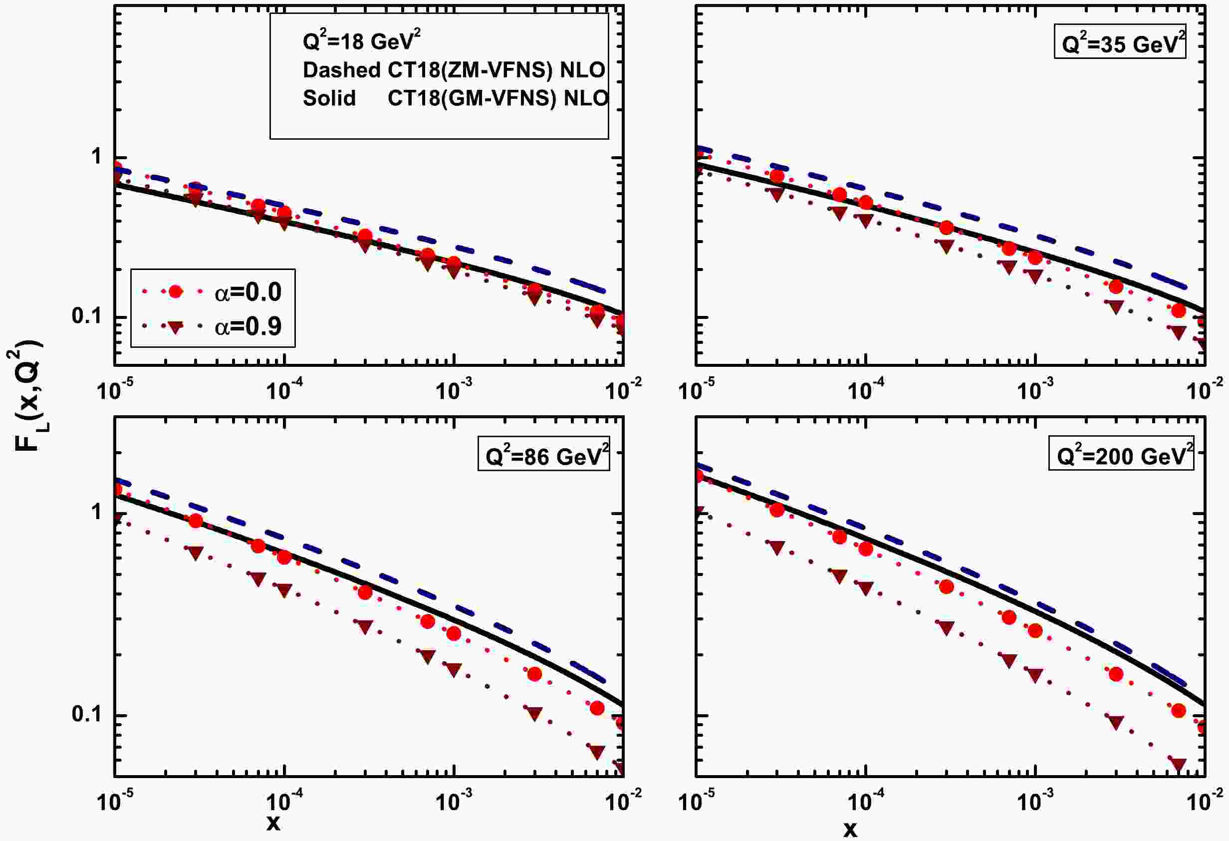
The x-dependence of the longitudinal structure function was calculated at several fixed values of $ Q^2 $ corresponding to H1-Collaboration data in a wide range of the expansion point $ z = \alpha $. Results are presented in Fig. 1, showing the x-evolution of $ F_{L}(x,Q^2) $ for $ \alpha = 0.0 $ (red circles) and $ \alpha = 0.9 $ (brown down-triangles). Clearly, for moderate and large values of the presented $ Q^2 $, the extracted longitudinal structure function within the NLO approximation aligns much better with the CT18 parametrization model at $ \alpha{\simeq}0.0 $. We determined that selecting $ \alpha\sim 0.0 $ as the expansion points for moderate and high $ Q^2 $ values yields sufficiently accurate results for our purposes.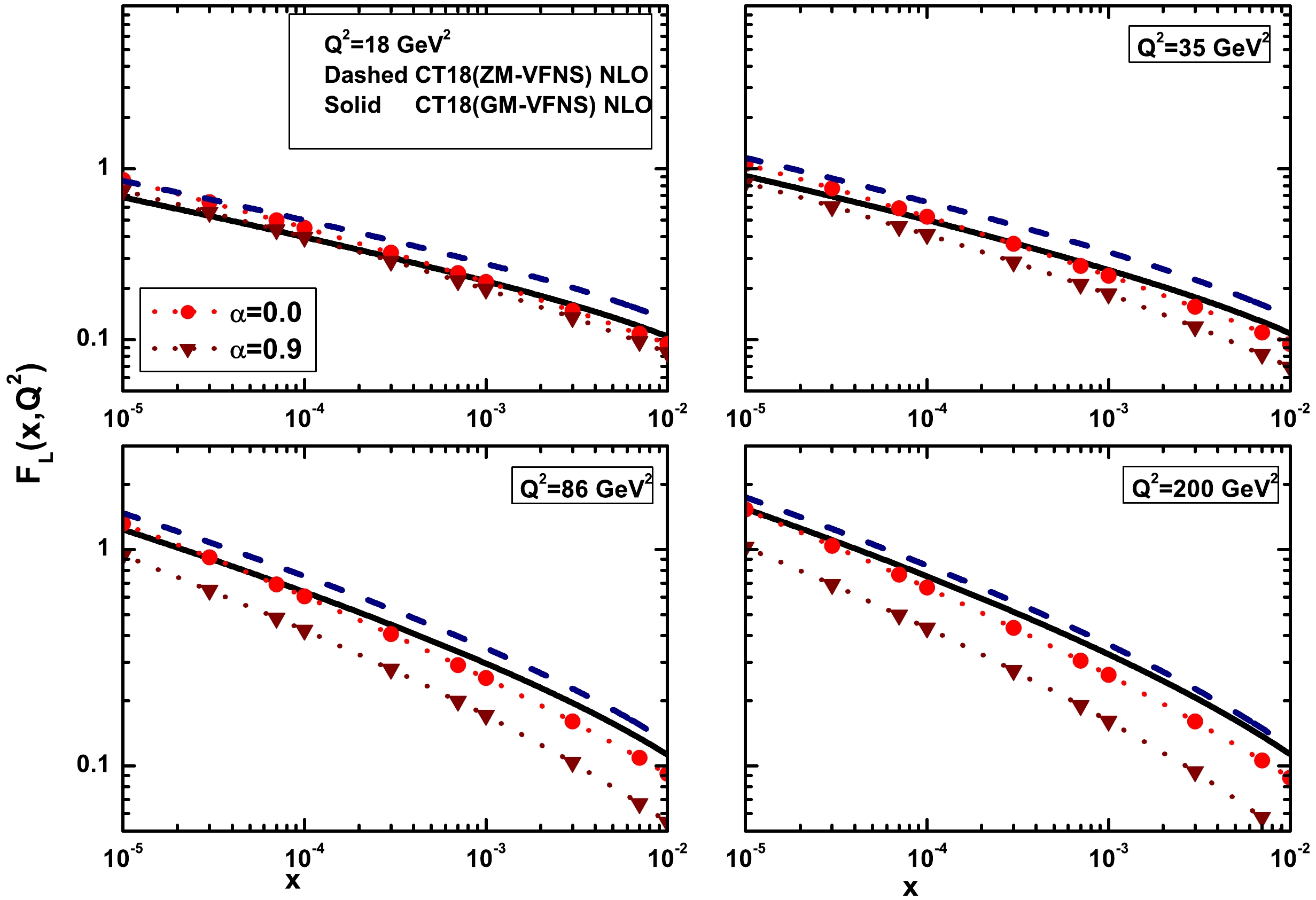

Figure 1.  (color online) The longitudinal structure function $ F_{L}(x,Q^2) $ plotted at fixed $ Q^2 $ as a function of x variable for $ \alpha = 0.0 $ (red circles) and $ \alpha = 0.9 $ (brown down-triangles), compared with the CT18 parametrization method [31] in GM-VFNS (solid curves) and in ZM-VFNS (dashed curves) at the NLO approximation.

In Fig. 2, the x dependence of the longitudinal structure function at $ Q^2 = 4.5 $ and $ 8.5\; \mathrm{GeV}^2 $ is compared with the H1 Collaboration data [15] along with total errors and the results from the CT18 (GM-VFNS) NLO parametrization model. Considering the expansion points ($ \alpha = 0.0 $ (blue squares), $ \alpha = 0.5 $ (green down-triangles) and $ \alpha = 0.9 $ (brown up-triangles)) used in the gluon density, the extracted longitudinal structure functions within the NLO approximation are comparable to the experimental data and the results of the CT18 NLO model.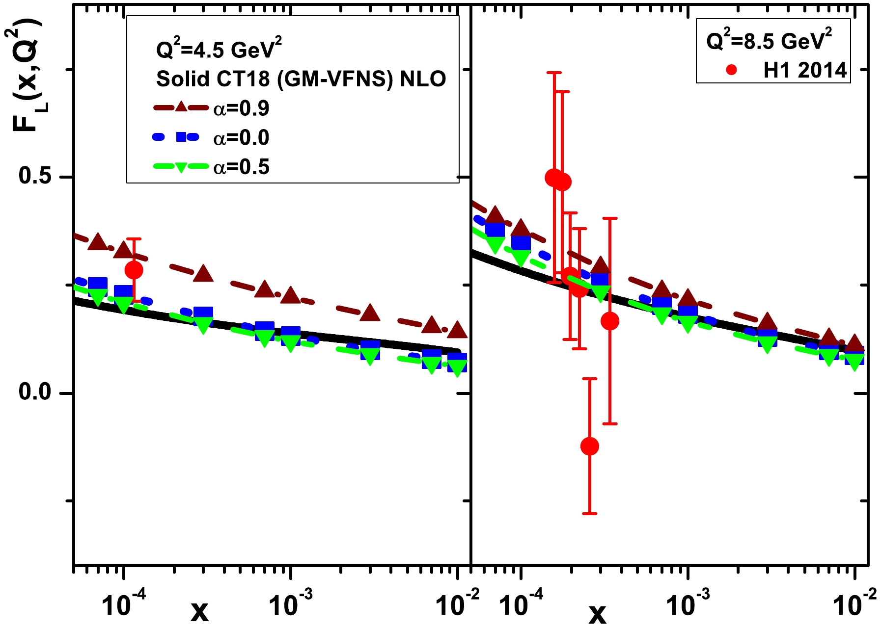

Figure 2.  (color online) The longitudinal structure functions at the NLO approximation with respect to the expansion points ($ \alpha = 0.0 $ (blue squares), $ \alpha = 0.5 $ (green down-triangles) and $ \alpha = 0.9 $ (brown up-triangles)) extracted and compared with the H1 experimental data (red circules) [15] along with total errors and the results of the CT18 NLO [31] parametrization model.

The H1 data for $ Q^2 = 4.5\; \mathrm{GeV}^2 $ were obtained by averaging the $ F_{L} $ data from Table 6 of [15] at the specified values of $ Q^2 $ and x. We observe that at low values of $ Q^2 $, the longitudinal structure functions across a wide range of expansion points align with the H1 data, along with their total errors. Comparing with the CT18 parametrization model, the longitudinal structure functions are similar at the expansion points $ \alpha{\lesssim}0.5 $.

In Fig. 3, the $ Q^2 $ dependence of the longitudinal structure function at small x of the NLO approximation is shown, with fixed values of the invariant mass W set at $ W = 230\; \mathrm{GeV} $. The results of calculations at the expansion point $ \alpha = 0.5 $ are presented and compared with the data from H1 Collaboration [15], along with total errors and the results of the CT18 parametrization method [31]. The extracted uncertainties are due to errors in the coefficients listed in Table 1. However, the extracted values in a wide range of expansion points are in good agreement with experimental data at both low and high $ Q^2 $ values.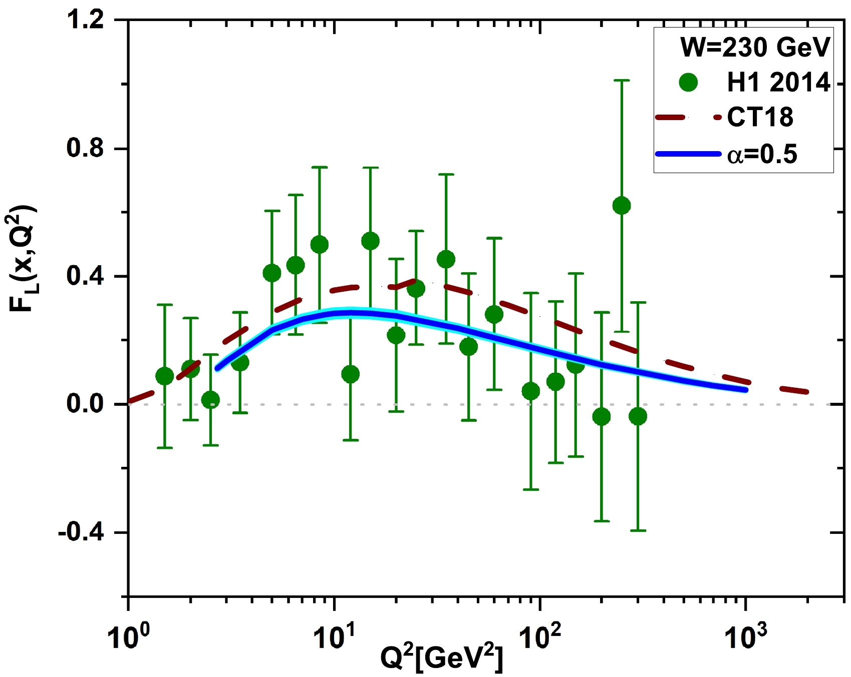

Figure 3.  (color online) The longitudinal structure functions $ F_{L}(x,Q^2) $ are extracted at a fixed value of the invariant mass W of $ 230\; \mathrm{GeV} $ at the expansion point $ \alpha = 0.5 $ (blue curve) with uncertainties and compared with data from the H1 Collaboration [15] along with total errors and the results of the CT18 parametrization method [31] (brown dashed curve).

Indeed, the longitudinal structure function results, according to the expansion method, strongly depend on the expansion points. However, the DIS-scheme splitting and coefficient functions for electromagnetic deep inelastic scattering with small x in an NLO fixed order expansion can be improved using the small x resummations, as described in [32, 33].

In conclusion, we have presented a method based on expanding the gluon density, to determine the longitudinal structure function of the NLO approximation at low x. This method relies on the momentum carried by the gluon density as a result of the expansion points within a kinematic region characterized by low values of the Bjorken variable x. We found that the expansion method of the gluon density provides the correct behavior of the extracted longitudinal structure function $ F_{L}(x,Q^2) $ at both low and high $ Q^2 $ values of the expansion points. Our results for $ F_{L}(x,Q^2) $are comparable with the data from the H1 Collaboration, those of the CT18 parametrization method, and the results obtained using the momentum space method [34].