Model for Glauber-type calculations of beam fragmentation at low energies

In experimental nuclear studies, the in-flight method is widely used for radioactive ion beam production. The primary beam is used to generate a specific nucleus in a target, and this nucleus is separated from other products in a fragment separator. To operate the fragment separator effectively, knowledge of the longitudinal momentum distributions of the nucleus is important.

Many nuclear research centers are producing low-energy ($ E<100 $ $A\cdot$MeV) radioactive beams using the in-flight method, such as FLNR (JINR, Russia) [1], FRIB (Michigan State University, USA) [2], GANIL (France) [3], RNC (RIKEN, Japan) [4], and INFN-LNS (Italy) [5]. This energy range allows studies of exotic nuclear structures in direct reactions.

Experimental data show a significant qualitative difference between the momentum distributions of fragments obtained at low energies and those obtained at higher energies. The distributions exhibit asymmetry, and the position of the maximum of each distribution changes with different fragments. In this context, understanding the fragmentation mechanisms is particularly important.

The in-flight method is based on the assumption that the longitudinal momentum ($ P_{\rm beam} $) distributions of the fragments are narrow and focused around the longitudinal momentum corresponding to the beam velocity. This study demonstrates that, at low energies, the longitudinal momenta of the fragments may significantly deviate from $ P_{\rm beam} $. Thus, an approach that relates the width and position of the peak of the longitudinal momentum distribution to the transferred momentum is required. The following example illustrates this problem. At an energy of 30 $A\cdot$MeV, which is typical for the beams in FLNR, the longitudinal emittence of the initial beam (2%) increases to approximately 20% after fragmentation [1], and the fragments are accepted into the secondary beam within a narrow region of the longitudinal momentum distribution. The optimal acceptance is achieved when the momenta of the fragments are close to the peak of the longitudinal momentum distribution [6].

The Glauber model is the most widely used approach for these types of calculations, as it provides a satisfactory description of experimental data at intermediate and high energies ($ E>100 $ $A\cdot$MeV). However, at energies below $ 100 $ $A\cdot$MeV, the applicability of the Glauber model becomes dubious. Therefore, in this study, experimental data on nuclear fragmentation at energies $ E<100 $ $A\cdot$MeV are accumulated, different parametrizations for describing the energies and angular distributions of the fragments are derived, and a simple model of the Glauber type is extended to allow calculations at low energies, for which the transferred momentum and beam momentum are of the same order of magnitude. The proposed approach accounts for energy and momentum conservation while maintaining simplicity and transparency.

This approach enables an analytical expression for the amplitude of the process to be derived. It also facilitates the correction of the amplitude via the Lorentz-invariant phase volume, thus accounting for energy and momentum conservation.

In this study, we introduce this model, analyze the scope of its applicability, and apply it to calculations of ¹¹B fragmentation in a Be target.

The element ¹¹B has the lightest nucleus of which a removal process involving a few protons produces ¹⁰Be, ⁹Li, and ⁸He fragments. All these nuclear fragments have been thoroughly studied experimentally; thus, we use them as input parameters for our approach. We analyze the changes in the phase volume and the longitudinal momentum distributions as functions of the beam energy and mass number of the fragments. We then compare the momentum distributions to those systematically obtained via widely used fragmentation calculations (see Refs. [7, 8]).

All the calculations of the momentum distributions and cross sections are performed using the Monte Carlo method.

In the general case, the differential cross section of a process with n bodies in the final state is expressed as

where T denotes the T-matrix, v represents the beam velocity, and ${\rm d}V^{(n)}$ denotes the phase volume of the n-body system of fragments.

We propose an approach in which we use the inelastic scattering amplitude obtained in the Glauber method (instead of the T-matrix) while preserving the Lorentz-invariant phase volume. Using this procedure, we formally incorporate conservation of energy and momentum; however, this provides only a qualitative description of the correlations and momentum distributions. Nevertheless, such an approach can describe the influence of the Q-value and other purely kinematical effects (which may be significant at low energies) on the momentum distribution of the fragments.

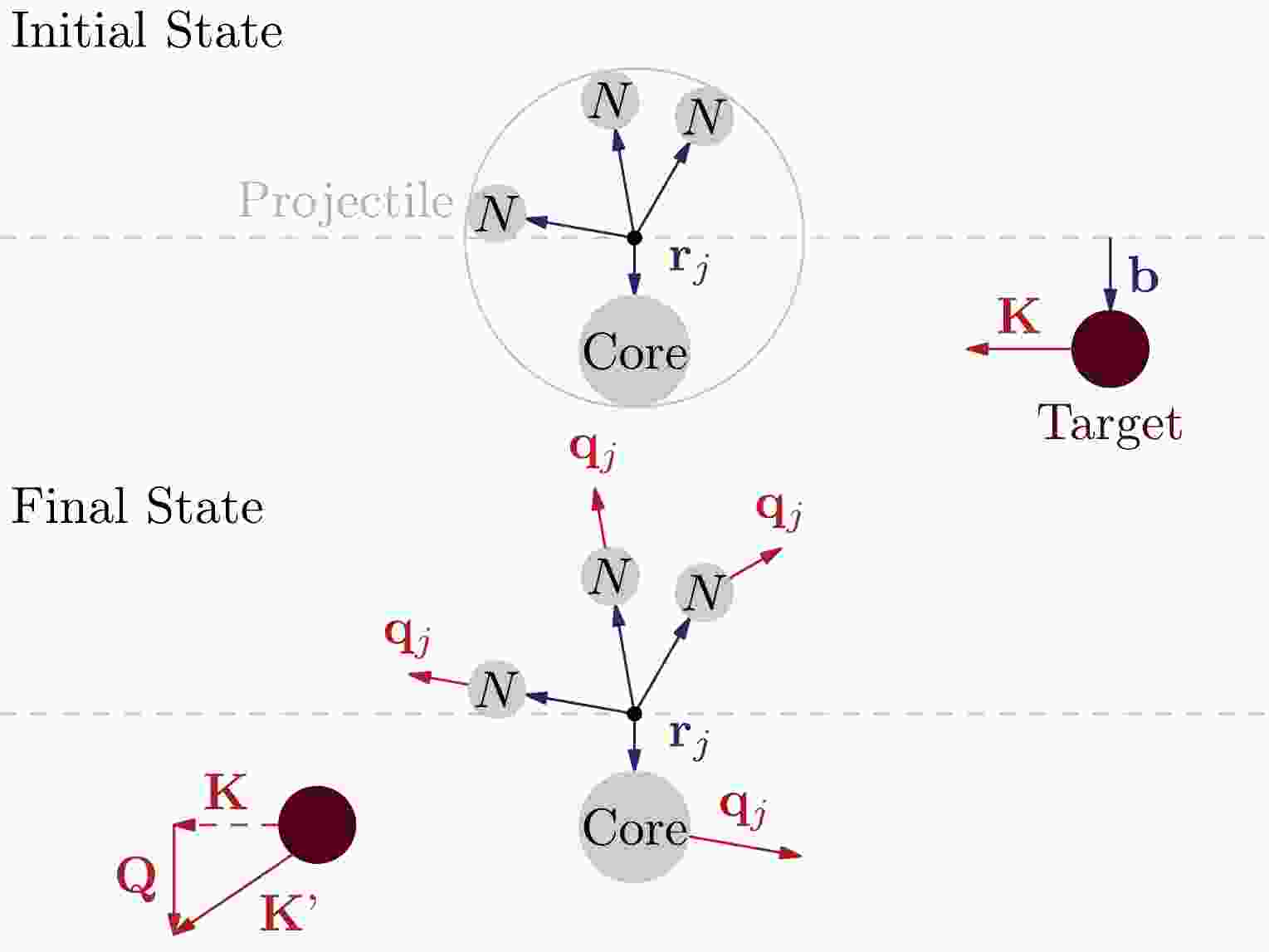
We now consider the fragmentation of a projectile (P) in a target (T) (Fig. 1) in the projectile's rest frame, assuming that the projectile consists of n fragments, which are composed of a relatively heavy core (C) and nucleons.

Figure 1.  (color online) Kinematical scheme of the fragmentation reaction and kinematical variables in the projectile's rest frame.

The inelastic scattering amplitude of this process can be derived using the integral over the impact parameter (${\bf{b}}$) and the coordinates of the preformed clusters (${\bf{r}}_j$); it can be expressed as

where $S_j$ is the profile function of the fragment-target (core-target $j=C$ and nucleon-target $j=N$) interaction obtained using the optical model potential (see Eq. (9)), ${\bf{t}}_j$ is the projection of ${\bf{r}}_{j}$ onto the impact parameter plain (orthogonal to ${\bf{K}}$) and is expressed as

$\Psi_I$ is the projectile's initial state wave function (WF) for the relative motion of the fragments with coordinates $ {\bf{r}}_j $ (the index j denotes the core and nucleon fragments) and is expressed as

$\Psi_F$ is the final state WF defined by the coordinates and momenta of the fragments:

Because we are considering the problem in the projectile's rest frame, ${\bf{K}}$ and ${\bf{K}}'$ are the initial and final target momenta, respectively; ${\bf{Q}}$ represents the target transferred momentum; and ${\bf{q}}_j$ represents the momenta of the fragments after being scattered in the projectile's rest frame (${\bf{q}}_j$ can also be interpreted as the transferred momenta of the fragments).

Using the single scattering approximation shown in Eq. (2), we obtain the sum

where $f_{j}({\bf{Q}})$ is the fragment-target elastic scattering amplitude [9]. In the transparent nucleon limit ($ S_N=1 $), Eq. (3) reduces to

Our next assumption concerns the factorization of the WFs of the initial state,

and final state,

Introducing the functions

and assuming that the final state WF can be approximated using plane waves, we obtain

Substituting Eq. (6) into Eq. (4) gives the amplitude of inelastic scattering:

The momenta ${\bf{Q}}$ and ${\bf{q}}_j$ in Eq. (2) are assumed to lie in the plane orthogonal to the momentum ${\bf{K}}$. However, if we assume $F_j$ and the core-fragment potential are centrosymmetric, the dependence of $\mathcal{F}_{if}$ on the directions of ${\bf{Q}}$ and ${\bf{q}}_j$ should be minimal, rendering the use of Eq. (7) reasonable.

$ F_C $ and $ F_N $ in Eq. (7) represent the form factors determined by the size of the nucleus. Thus, the amplitude of inelastic scattering is defined by the elastic scattering amplitude of the core $ f_{C}({\bf{Q}}) $.

Using the oscillator WF, which is expressed as

we obtain the expression for the form factors $F_j$

where $\langle r_j\rangle$ is the root mean square (RMS) distance of fragment j from the center of mass of the projectile.

The parameters of this approach include the RMS radii of the fragments and the corresponding RMS distance between each fragment and the center of mass of the projectile.

The elastic scattering amplitudes $f_{C}({\bf{Q}})$ and $f_{N}({\bf{Q}})$ are calculated in the Glauber model using the corresponding core-target profile function $S_j$.

In our calculations, the profile functions of the core-target interaction are derived using the model potential, which is expressed as

where $r = \sqrt{b^2+z^2}$, $V_{j}(r)$ denotes the optical model potential for the core-target or nucleon-target interaction, b is the impact parameter of the center of mass of the fragment (see, for example, Refs. [10, 11]), v is the beam velocity, and z is the coordinate along the beam axis.

To perform the calculations over a wide energy range (10-100 $A\cdot$MeV), we use the standard parametrization of the nucleon-nucleon interaction potential with the parameters from Refs. [12, 13], which are valid for incident energies ranging from 10 to 2000 $A\cdot$MeV. The optical potential of the core-target interaction can be found by folding [14] the potential with the core density distribution.

The core-target interaction potential is expressed as

where $A_{C}$ is the core mass number, $\rho_{C}$ denotes the core density distribution, and $ \overline{V_{C}}(|{\bf{r}} - {\bf{r'}}|)$ represents the effective interaction potential. In addition,

The density distributions of the interacting nuclear systems are approximated by the Gaussian distribution [15] as

where $ \alpha = \left[\frac{2}{3} \langle r^2 \rangle \right]^{-1} $is the density distribution parameter related to the RMS radius of the nucleus ($ \langle r^2 \rangle^{1/2} $),$ \rho(x) $ is normalized to unity, and $ \overline{\sigma}_{NN} $ is the nucleon-nucleon cross section averaged over the number of neutrons and protons involved in the interaction (for more details see Refs. [12, 13]).

For the fragmentation of ¹¹B, we considered three reactions leading to production of the ¹⁰Be, ⁹Li, and ⁸He isotopes:

These reactions illustrate the "path" toward the neutron dripline. Calculations were performed for the beam energies of 10, 30, and 100 $A\cdot$MeV, probing the changes in the differential elastic cross section and the longitudinal momentum distributions of the core fragment as functions of the incident energy. The Monte Carlo method was used to calculate the corresponding momentum distributions.

Figure 2 displays the differential elastic cross section as a function of the transferred momenta$ q_j $ for the protons ($ j=p $) and core fragments ($ j=C $, where C corresponds to ¹⁰Be, ⁹Li, and ⁸He) in a Be target for the incident energies of 10, 30, and 100 $A\cdot$MeV. The calculated proton cross sections were smaller than the core cross sections by a few orders of magnitude. The corresponding amplitudes satisfied $f_C\gg f_N$, indicating that the core-target interaction dominated over the nucleon-target interaction. Furthermore, Fig. 2 shows that when the nucleon transfer occurred, the momentum transfer significantly exceeded the value corresponding to the first diffraction minimum. In the calculations of the elastic scattering, we assumed that the dominant contribution to the elastic scattering cross section corresponded to the transferred momenta that were smaller than those at the first diffraction minimum (see Fig. 2).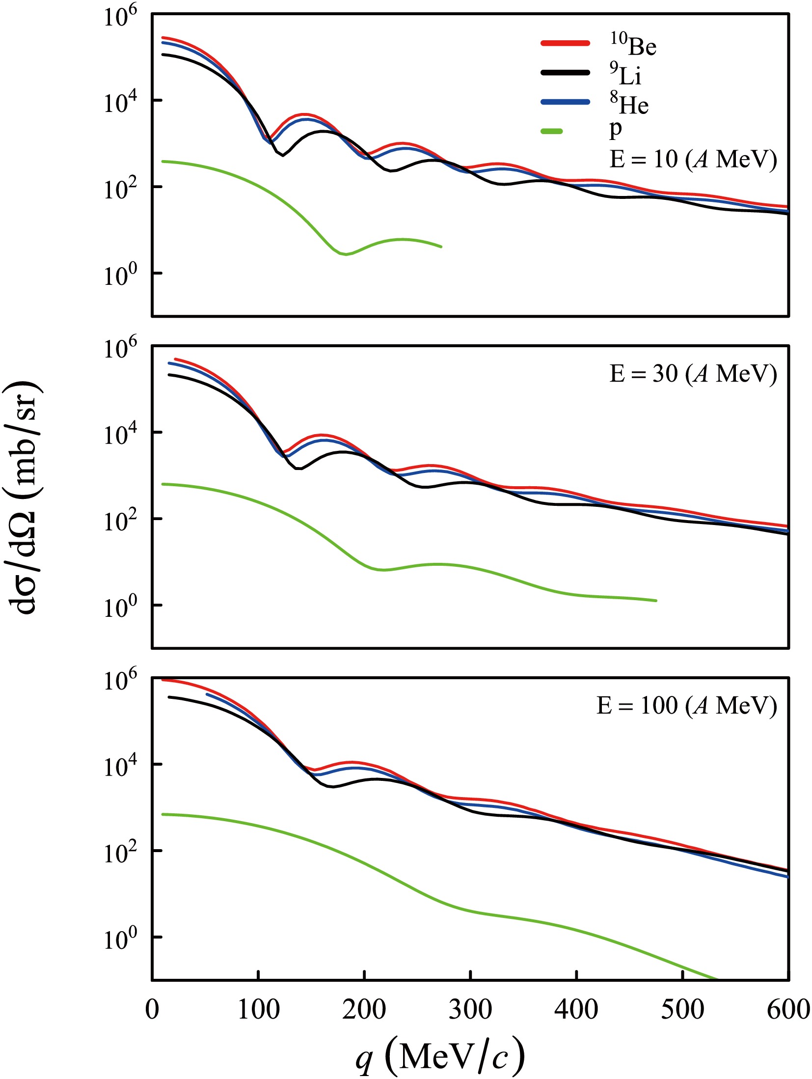

Figure 2.  (color online) Differential elastic scattering cross sections as functions of the transferred momenta q for protons and heavy ions (¹⁰Be, ⁹Li, and ⁸He) scattered on a ⁹Be target at different projectile energies (see legends in the panels).

In our model, the projectile nucleus ¹¹B is treated as a system of a pre-formed heavy cluster and valence protons. The structure of ¹¹B is characterized by the form factor $ F_C({\bf{q}}_C) $ described in Eq. (8), which is determined by the RMS distance of the core in ¹¹B. In our calculations, we used the RMS distance of the proton, $ \langle r_{p} \rangle = 2.43\; \mathrm{fm} $, which was determined by the standard charge radius systematics, $ 1.2 \times A^{1/3} $. As a first approximation, the RMS distance of the core ($\langle r_C \rangle$) can be calculated assuming a point particle.

In the general case, the core WF in ¹¹B may be more complex, resulting in variations in $\langle r_C \rangle$. To demonstrate the sensitivity of our results to this parameter, we varied $\langle r_C \rangle$ (see Table 1) from the minimal value (corresponding to a more central impact) to the maximal value (representing a more peripheral interaction). The values of $\langle r_C \rangle$ are presented in the Table 1.

Fragment	$\langle r_c \rangle$	$\min\langle r_c \rangle$	$\max\langle r_c \rangle$
10Be	0.24	0.12	0.49
9Li	0.49	0.24	0.97
8He	0.73	0.36	1.46

Table 1.  RMS distances of the heavy fragments used in the calculations, where $\langle r_c \rangle$ is the default value, $\min\langle r_c \rangle$ represents the radius of the "more central" reaction, and $\max\langle r_c \rangle$ represents the radius of the "more peripheral" reaction. All values are given in fm.

Figure 3 shows the correlation plots of the target transferred momentum (Q) versus the projection $q_{Cz}$ of the core momentum $q_C$ onto the z-axis, coinciding with the beam direction. The calculations were performed for beam energies of 10, 30, and 100 $A\cdot$MeV and for different core fragments of ¹⁰Be, ⁹Li, and ⁸He.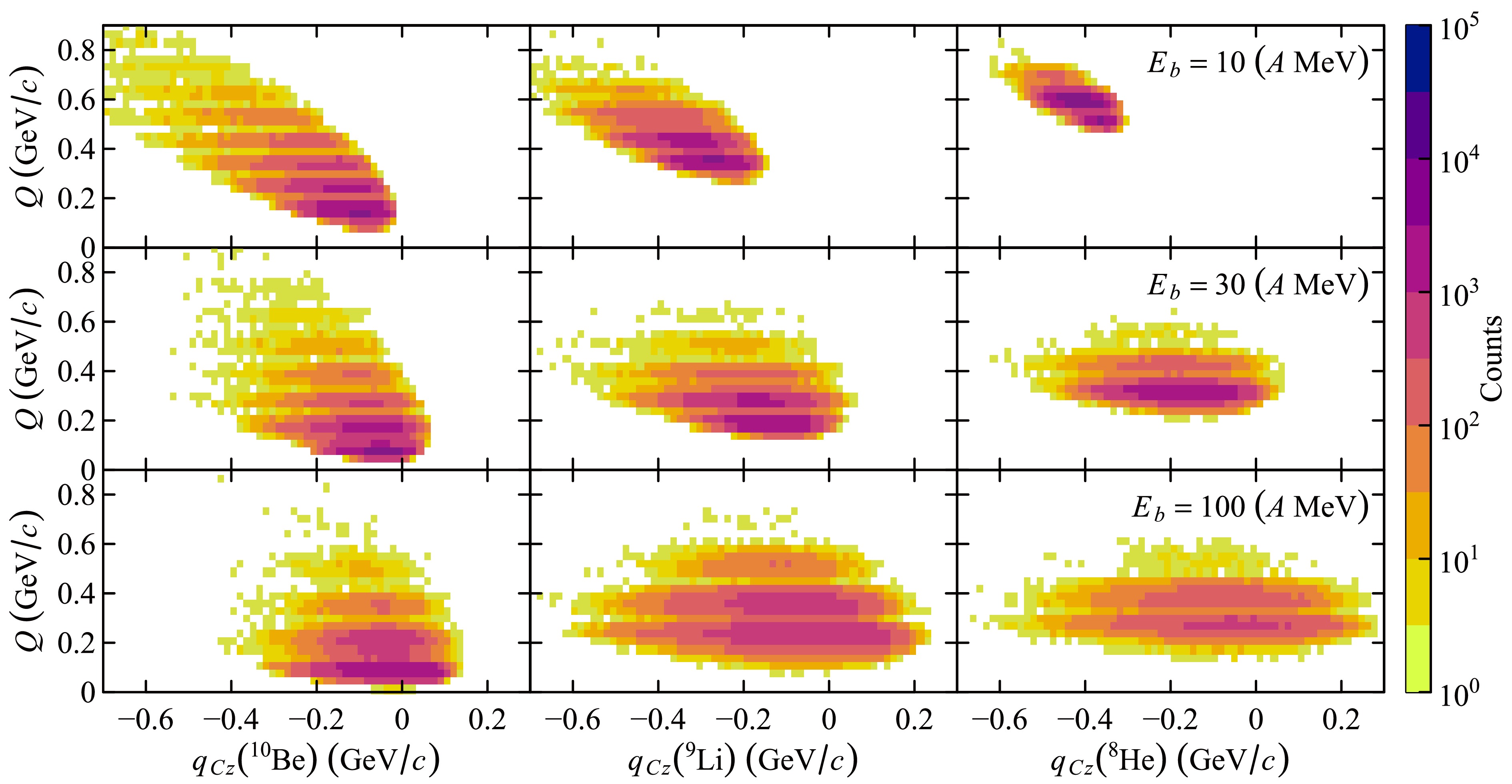

Figure 3.  (color online) Correlation between the transferred momentum of the target (Q) and the longitudinal component of the core momentum ($q_{Cz}$) in the projectile's rest frame, obtained using the Monte Carlo method for different fragments (columns) and ¹¹B beam energies (rows). The color scale indicates the number of events in the Monte Carlo calculations.

At low beam energies (10 and 30 $A\cdot$MeV), Q and $q_{Cz}$ exhibited a strong correlation, which weakened as more nucleons were removed.

The kinematic locus included only non-zeroth transferred momentum Q because part of the beam energy was spent on nucleon knock-out. Therefore, the Serber model [16], which is valid in the $Q=0$ MeV/c limit, was not applicable in this case, and the core fragments appeared to move slower than the beam nuclei. The Serber model describes the fragmentation process as a sudden removal of nucleons from the nucleus. In this model, the longitudinal momentum distribution of the fragments is determined by the initial WF of the system, represented by the form factor of the initial state. For the case in which $Q\ll q_C$, Eq. (7) reduces to the Serber model.

At high energy (100 $A\cdot$MeV), the effect of "slowing down" was less pronounced, and the correlation became more symmetric with respect to $q_{Cz}=0$, approaching the predictions of the Serber model. However, the $Q\ll q_C$ case was still not realized. In future work, we plan to investigate the kinematic conditions under which our approach is reduced to the Serber model.

In Fig. 4, we present the correlation between the two projections of the core momentum in the projectile's rest frame ($q_{Cx}$ and $q_{Cz}$).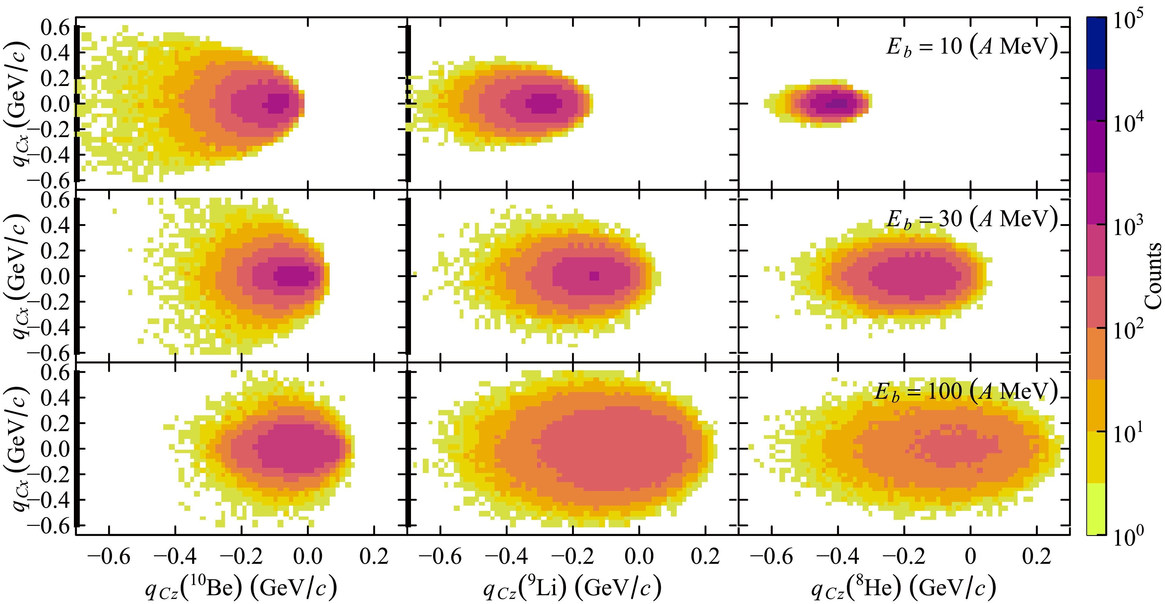

Figure 4.  (color online) Correlation between the transverse ($q_{Cx}$) and longitudinal ($q_{Cz}$) components of the core momentum in the projectile's rest frame, obtained using the Monte Carlo method. The layout is the same as that in Fig. 3. The color scale indicates the number of events in the Monte Carlo calculations.

In these plots, the kinematical loci of the fragments are clearly visible, and the loci of $q_{Cz}$ are asymmetric relative to the momentum of the beam ($q_{Cz}=0$). This indicates that the fragments tended to "slow down" at low energies relative to the beam velocity, which is a phenomenon related to the reaction kinematics.

This result demonstrates that the shape of the longitudinal momentum distributions changed significantly as the beam energy varied, highlighting the importance of considering momentum and energy conservation. From this perspective, the models that assume a sudden removal with $Q \to 0$, such as the Serber model and the traditional eikonal approximation of the Glauber model, provide only a qualitative description of the momentum distributions. At high energies, these models offer an adequate quantitative description of the cross sections; however, at energies below 100 $A\cdot$MeV, they do not provide an accurate description of the momentum distributions.

At higher energies, for which the transferred momentum is much smaller than the beam momentum and is thus negligible, the results of our model approached those obtained by the Glauber model in the transparent proton limit.

The sensitivity of our calculations to $\langle r_C\rangle$ is illustrated in Fig. 5, which presents the characteristics of the longitudinal momentum distributions, such as the peak position, standard deviation (SD), and skewness of the $q_{Cz}$ distribution.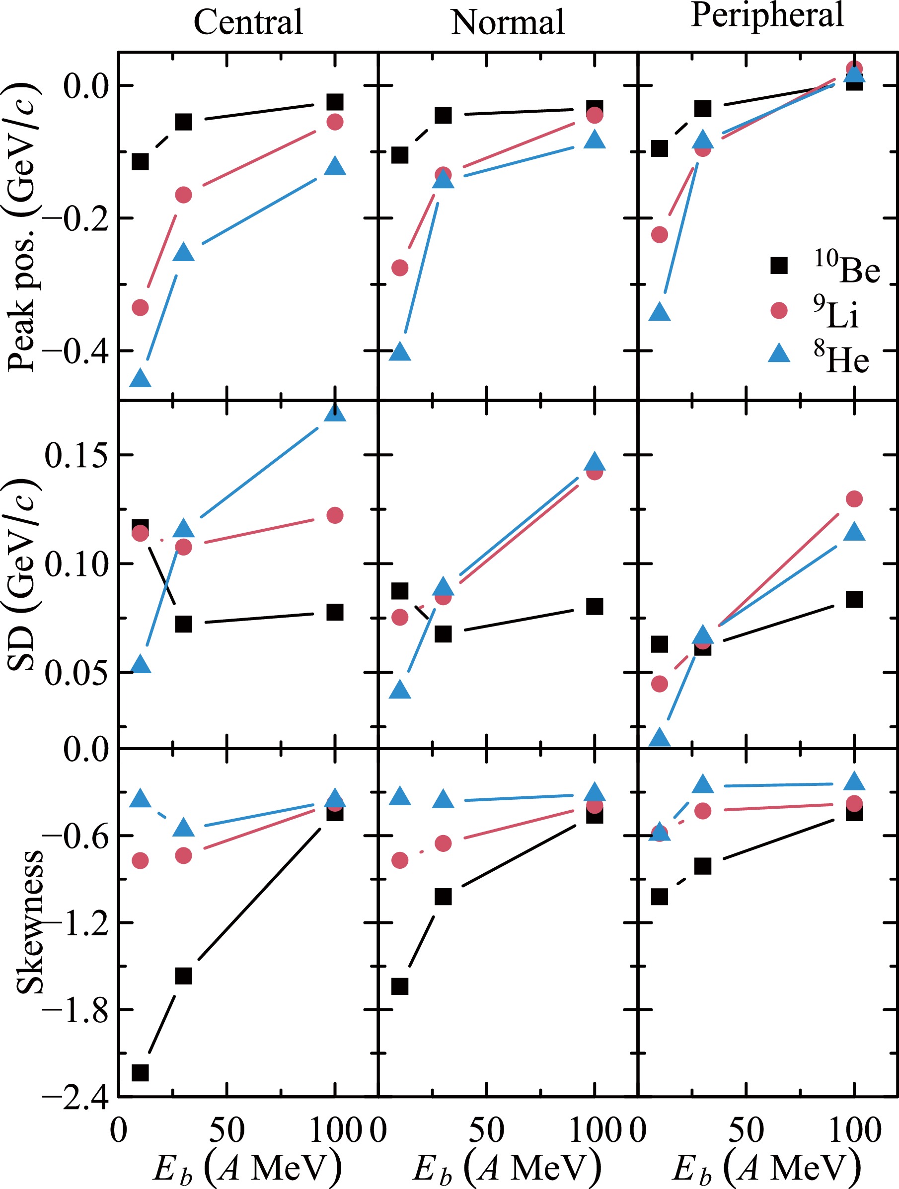

Figure 5.  (color online) Mode (peak position), standard deviation (SD), and skewness for different values of $\langle r_C\rangle$ (see Table 1).

As the mass of the fragment increased, the peak position in the momentum distributions shifted to higher values and the skewness decreased. The standard deviation of the longitudinal momentum distribution varied depending on the type of fragment.

The plots indicate that in peripheral reactions, the fragment moved faster than the projectile. Additionally, the $q_{Cz}$ distribution narrowed. In central interactions, the $q_{Cz}$ distribution became wider and more asymmetric. Thus, more peripheral reactions produced faster fragments, whereas more central reactions produced fragments that were relatively slow compared to the beam velocity.

Finally, Fig. 6 compares the calculated widths of the longitudinal momentum distributions of the fragments to the predictions of the widely used Goldhaber model [7]. Following the approach outlined in this article, the standard deviation can be expressed as

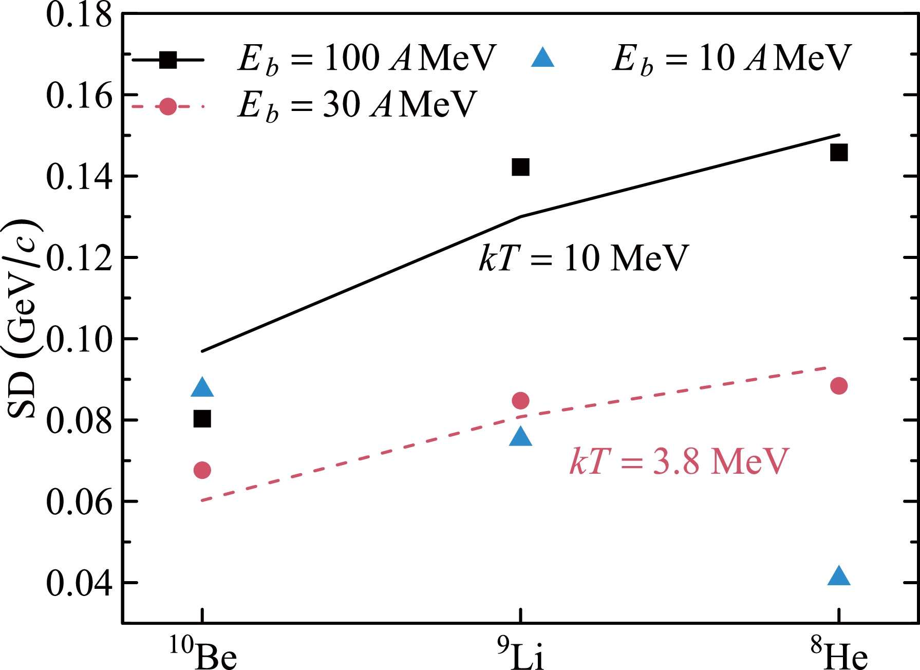
Figure 6.  (color online) Comparison between the standard deviation (SD) of $q_{Cz}$ obtained in our calculations (points) and the predictions of the model from Ref. [7] (lines). The values of $kT$ for the beam energies of $E_b=100$ A MeV and $E_b=30$ A MeV are shown in the panels.

where A is the mass of the incident ¹¹B particle and K is the mass of the fragment (¹⁰Be, ⁹Li, and ⁸He). The temperature T and Boltzmann constant k jointly define $ \sigma^2 $, which describes both the mean excitation energy transferred to the fragment during nuclear decay and the width of the momentum distribution of the fragment.

For high beam energy ($E_b=100 \;\;A\cdot{\rm{ MeV}}$ and $E_b=30 \;\;A\cdot{\rm{ MeV}}$, our results exhibited reasonable agreement with the predictions of Ref. [7]. For low beam energy ($E_b=10 \;\;A\cdot{\rm{ MeV}}$), the dependence of the widths of the longitudinal momentum distributions on the fragment mass number obtained via our calculations qualitatively differed from that in Ref. [7], highlighting the limitations of the Goldhaber model and emphasizing the applicability of our proposed approach.

In this study, we proposed a new nuclear fragmentation model based on the Glauber model, which we modified to account for energy and momentum conservation.

Using the example of ¹¹B fragmentation, we calculated the longitudinal momentum distributions of the ¹⁰Be, ⁹Li, and ⁸He fragments. All results were obtained within the transparent proton limit. At energies above $100 \, A\cdot\text{MeV}$, our model produced results similar to those obtained by the eikonal approximation of the Glauber model in the transparent proton limit ($S_N=1$). Additionally, the precision of the proposed approach improved as the heavy fragment mass increased.

At low energies, the peak position of the longitudinal momentum distribution increased as the core mass decreased. In addition, at energies below $100 \, A\cdot\text{MeV}$, the fragments moved slower than the beam nuclei, as defined by the kinematic locus, whereas at higher energies ($E > 100 \, A\cdot\text{MeV}$), the fragments moved either faster or slower depending on the reaction geometry.

Accounting for energy and momentum conservation led to significant changes (i.e., asymmetry) in the shape of the longitudinal momentum distributions, producing a low-momentum tail owing to the large transferred momentum. Thus, compared to the Glauber model, our approach describes fragmentation over a wider range of momentum transfer values.

A comparison with calculations from other models and parametrizations indicated that at energies below 100 $ A\cdot\text{MeV}$, kinematical loci as well as energy and momentum conservation must be taken into account when planning experiments and determining optimal conditions for fragment production.