Inferring a spinning black hole in an expanding universe via the S2 star around the Galactic Center

As a pivotal prediction of general relativity, black holes have significantly enhanced our grasp of gravitational physics. Over recent decades, major strides in black hole physics research and concrete evidence have firmly established their existence, leading to unparalleled scientific advancements. Penrose masterfully used mathematical methods to validate the widespread presence of black holes across the cosmos [1]. The landmark 2015 detection of gravitational waves from binary black holes merge by LIGO [2], the revealing images of the supermassive compact objects M87$ ^\star $ [3] and Sagittarius A$ ^\star $ (Sgr A$ ^\star $) [4] at the heart of the M87 galaxy and the Milky Way captured by the Event Horizon Telescope Collaboration, and the detailed long-term monitoring of stellar orbits around the supermassive compact object at the Milky Way's center by the GRAVITY collaboration [5, 6], all collectively form a robust array of astronomical evidence underpinning the existence of black holes.

In contemporary astrophysics, the enigmatic nature of black holes presents a profound puzzle, with Sgr A$ ^\star $, the closest known black hole to Earth, standing at the forefront of this exploration. Its intense gravitational field provides a unique opportunity to probe the fundamental mysteries of black holes, making Sgr A$ ^\star $ an exceptional astrophysical laboratory [7]. Research initiatives have focused on exploring phenomena that challenge the conventional framework of general relativity, particularly through the study of orbital motions of S-stars orbiting Sgr A$ ^\star $, which provide critical insights into its intrinsic properties [8]. Among these, the S2 star is particularly interesting due to its short orbital period of approximately 16 years and high eccentricity of around 0.88 [9]. Such a star has a pericentric distance of 120 A.U. $ \approx $ 1400 Schwarzschild radius, and an orbital velocity of 7650 km s$ ^{-1} $ at periapsis, which is close to 2.6% of the speed of light [10]. These special orbital characteristics of S2 stars make it a sensitive probe of the gravitational field in the Galactic center. Extensive research utilizing observational data from S2, including astrometric positions and radial velocities, has been conducted to dark matter [11−13]. Additionally, significant efforts have been dedicated to testing various theories of gravity [14−20]. Most of these studies were done on the basis that Sgr A$ ^\star $ is a non-spinning black hole.

However, certain observations suggest that Sgr A$ ^\star $ is spinning. Near-infrared periodic flares indicate a dimensionless spin parameter of approximately $ \chi = 0.52 $ [21], while X-ray flares suggest a higher spin, with a dimensionless spin close to $ \chi = 0.9939 $ [22, 23]. In recent years, the motion of photons in strong fields near spinning black holes and the black hole shadow have been extensively investigated [24−28]. Driven by these results, it is necessary to consider the black hole spin when exploring stars orbiting Sgr A$ ^\star $. Although the effect of spin is relatively weak, identifying its spin behavior could provide valuable insights for future research. Additionally, our universe is expanding at an accelerating rate [29, 30], making it crucial to account for spin gravitational sources in a dynamic universe when studying the motion of stars near supermassive black holes. However, understanding the universe's overall state through local observations remains extremely challenge.

To address this challenge, the Kerr-de Sitter spacetime background, which incorporates a positive cosmological constant as characterized in the Lambda Cold Dark Matter model, has garnered significant research interest [31−33]. This solution integrates the concept of an expanding universe into black hole physics. Beyond supernova observations, data from the cosmic microwave background also prefer the conclusion that the universe is expanding [34]. The cosmological constant, interpreted as dark energy [35], is one of the explanations for the driving force behind this expansion. Previous researches on the motion of photons in Kerr-de Sitter spacetime have provided clear explanations of photon behavior [36−38]. This paper aims to extend these studies by focusing on the motion of massive particles near a Kerr-de Sitter black hole. Specifically, we treat Sgr A$ ^\star $ as a Kerr-de Sitter black hole to investigate the effects of black hole spin and cosmic expansion on the motion of stars.

Early researchers explored the influence of black hole spin and the cosmological constant on orbital motion, calculating their effects on several specific orbits (S1, S2, S8, S12, S13, S14) [39, 40]. These researches showcased the orbital precession and the Lense-Thirring precession for certain dimensionless spin parameters, specifically $ \chi = 0.52 $ and $ \chi = 0.9939 $. However, the specific range within which black hole spin and the cosmological constant are applicable remains undetermined. Since then, nearly 20 years of additional observations have significantly enriched the data pool [5, 41]. Currently, astrometric position data for over a dozen stars have been published, along with their radial velocities obtained through spectroscopic measurements [41]. Among these stars, the S2 star is particularly notable for having two complete radial periods observed. Recently, the GRAVITY collaboration used the parameterized Newtonian approximation to determine the orbital precession of S2 star [9]. The publication of these data has inspired us to explore spacetime parameters through numerical simulations, applying the latest data to constrain Kerr-de Sitter black holes. In this paper, we focus on the Kerr-de Sitter black hole within the framework of general relativity. We employ Markov Chain Monte Carlo (MCMC) algorithm to investigate the effects of black hole spin and the cosmological constant on stellar orbits. Our findings may pave the way for further research into the dynamics of Kerr-de Sitter spacetime.

This paper is organized as follows. In Sec. 2, we introduce the basic concept of Kerr-de Sitter black hole and study the properties of orbital motions by geodesic equations in this spacetime. In Sec. 3, we explain our orbital model in detail and give corresponding observational corrections. In Sec. 4, we perform MCMC simulations to explore the parameters of the Kerr and Kerr-de Sitter black holes with publicly available astrometric and spectroscopic data of S2 star around Sgr A$ ^\star $. Finally, we summarize the research results in Sec. 5.

Kerr-de Sitter spacetime is a stationary and axially symmetric solution to Einstein's field equations in general relativity that describes the geometry around a spinning massive object in an expanding universe with a positive cosmological constant [42]. The cosmological constant $ \Lambda $ introduces a repulsive gravitational effect on large scales, causing the universe to expand. This expansion modifies the spacetime geometry around the spinning mass, leading to unique features compared to other solutions in general relativity [36, 43].

The Kerr-de Sitter metric in Boyer-Lindquist coordinates with the geometrized units $ (G = c =1) $ can be written in the following form [44, 45]:

where we use abbreviations

in which $ \Lambda > 0 $ is the cosmological constant, $ M $ is the mass of black hole and $ a $ is the spin of black hole per unit mass. For simplicity and clarity, we introduce a dimensionless black hole spin parameter $ \chi $, defined as $ \chi = a/M $. In this notation, $ \chi \in (-1, 1) $, where $ \chi > 0 $ indicates a counterclockwise spinning black hole, $ \chi = 0 $ represents a non-spinning black hole, and $ \chi < 0 $ signifies a clockwise spinning black hole, as viewed along the $ z $-axis. It is easy to find that the Kerr-de Sitter solution includes the Kerr $ (\Lambda = 0) $ solution, the Schwarzschild-de Sitter $ (a = 0) $ solution and the Schwarzschild $ (\Lambda = a = 0) $ solution as special case.

In Kerr-de Sitter spacetime, the horizons can be determined by solving $ \Delta_r=0 $. When $ \Lambda \neq 0 $, there are four horizons: the inner and outer horizons, the cosmological horizons far from the black hole and "inside" the singularity [36]. The detailed analysis of the horizon structure can be found in Refs. [44, 46, 47]. The $ g_{tt} $ component of the metric vanishes to yield the inner and outer infinite redshift surfaces [48]. The spacetime region between the outer event horizon and the outer infinite redshift surface constitutes the ergosphere, from which energy can be extracted via the Penrose process [49].

In stationary, axially symmetric spacetimes, the norm of the four-velocity remains constant due to parallel transport. Additionally, geodesic motion conserves both energy and angular momentum about the symmetry axis. However, these three constants alone are generally insufficient to fully simplify the geodesic equations. Carter resolved this problem by demonstrating the separability of the Hamilton-Jacobi equation and deriving an additional constant of motion [50]. As a result, the time-like geodesic equations in Kerr-de Sitter spacetime are completely integrable. We start with a Lagrangian for a free particle in the Kerr-de Sitter spacetime:

which represents the norm of the four-velocity, with $ 2 {\cal{L}} = 0 $ and $ -1 $ for massless and massive particles, respectively. The overdot here and in the rest of this section denotes differentiation with respect to the proper time $ \tau $. The stellar orbits around Sgr A$ ^\star $ are investigated in this paper, hence the choice of $ 2 {\cal{L}} = -1 $. Following the Lagrangian, the generalized momentum is $ p_\mu = \frac{\partial {\cal{L}}}{\partial \dot{x}^\nu} = g_{\mu \nu} \dot{x}^{\nu} $. Then, we can obtain the energy and $ z $ component of the angular momentum per unit mass of the motion are, respectively:

For the fourth constant, we will use the Hamiltonian to obtain it. In the standard way, the Hamiltonian is given as

substituting $ g^{tt} $, $ g^{\varphi \varphi} $, $ g^{t\varphi} $ into the above equation, we can separate the variables in it, reads as

where $ K $ stands for the constant of separation in the Hamilton-Jacobi equation [50]. By utilizing these four constants, the geodesic equations can be expressed in first-order form:

Due to the spin of Kerr-de Sitter black holes, it induces a dragging effect on spacetime, thereby influencing the orbital motion of celestial bodies around compact celestial objects. The orbital plane of orbiting celestial bodies undergoes precession [51], simultaneously impacting orbital precession as well. In the weak-field approximation, the impact of the black hole spin on orbital precession can be neglected, whereas its influence on the orbital plane precession—namely, Lense-Thirring precession—is quite significant. Stepanian et al. considered the influence of cosmological constant and obtained approximate formulas of orbital precession and Lense-Thirring precession [52, 53]. In the International System of Units, their respective expressions are:

where $ a_\star $ and $ e $ are the semi-major axis and the eccentricity of the orbit, respectively. Here, $ \Delta \omega $ represents the angle that periapsis shifts over one radial period, while $ \langle \dfrac{d \Omega'}{d t} \rangle $ denotes the average shifted rate of longitude of the ascending node defined within the stellar orbital plane with the equatorial plane of the black hole as the reference plane [54], $ \Omega' $ as depicted in Figure 1. Future observations on the orbital precession of other stars around Sgr A$ ^\star $, coupled with the detection of the Lense-Thirring precession, could provide significant constraints on the spin of Sgr A$ ^\star $ and offer substantial limitations on the cosmological constant.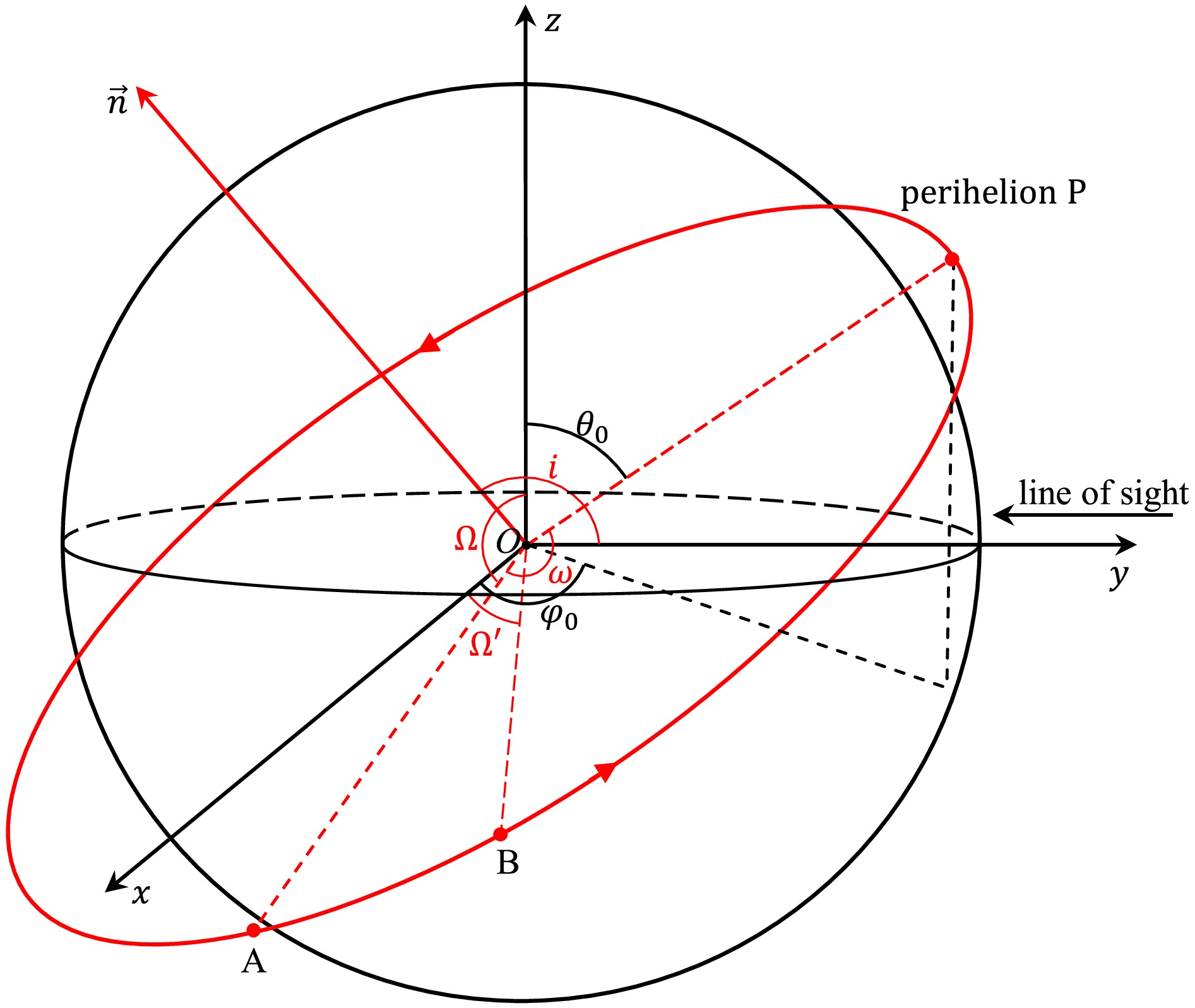

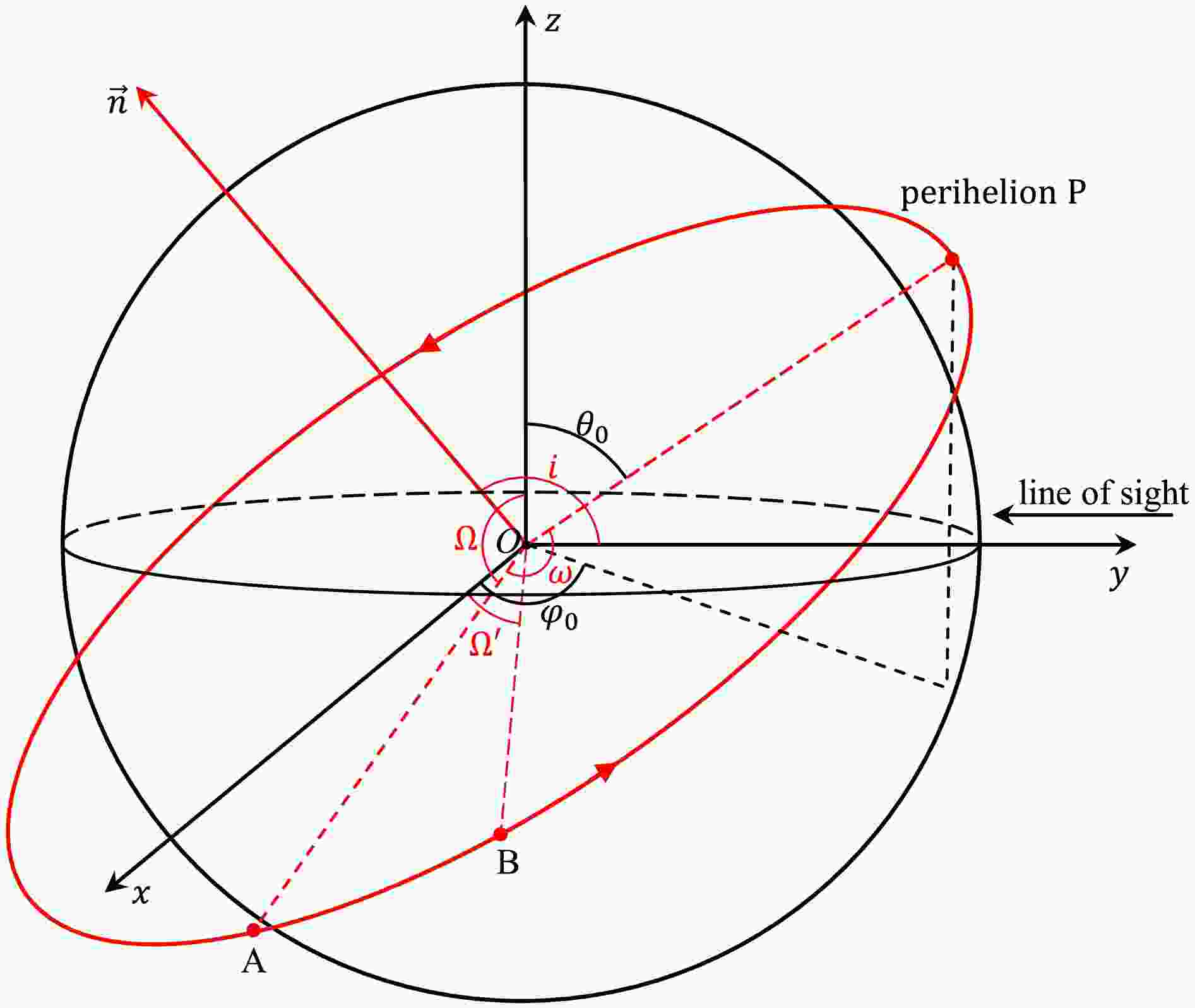
Figure 1.  (color online) Schematic diagram of orbital elements and coordinate [56], $ O $ is the origin of the coordinate. $ \vec{n} $ is the normal vector of the orbital plane. $ i $ is the angle between the line of sight and the normal vector to the orbital plane. $ \Omega $ is the position angle of the ascending node $ A $ in the $ xOz $ plane. $ \Omega' $ is the position angle of the ascending node $ B $ in the $ xOy $ plane. $ \omega $ is the angle between the line of ascending node $ A $ and the semi-major axis. $ (\theta_0, \varphi_0) $ are the spherical coordinates of perihelion $ P $.

In this section, we present the orbital motion of stars around a Kerr-de Sitter black hole and detail the numerical methods used for solving the relevant equations. We address the second-order geodesic equations (17) in a Cartesian coordinate system centered on the Galactic Center (illustrated in Figure 1), with initial conditions derived from Keplerian elements and projected using Thiele-Innes elements. Relativistic corrections, including Römer time delay (35), frequency shifts (38), and the motion of the solar system relative to the Galactic Center (as expressed in Eqs. (36), (37) and (42)), are applied to match observational data. Utilizing publicly available astrometric and spectroscopic data for the S2 star, which consists of 145 astrometric positions [41], 44 radial velocities [41], and orbital precession [9], we estimate the parameters outlined in Eq. (43) as well as spacetime parameters. This estimation is carried out using the MCMC algorithm, implemented through the $\mathrm{EMCEE}$ Python package, with the likelihood function as defined in equation (44).

The trajectory of a star orbiting a Kerr-de Sitter black hole is determined by a specific set of differential equations (11-14). While these equations are concise, the square roots in Eqs. (12) and (13) tend to accumulate errors at turning points during numerical integration. Additionally, manual adjustments to the signs of the $ \frac{dr}{d\tau} $ and $ \frac{d\theta}{d\tau} $ are required at each turning point. To circumvent these problems and harness astronomical observations more effectively, we choose to solve the second-order geodesic equations that take the derivative of $ t $ [16]. Inspired by Ref. [55], the geodesic equations can be converted to

Due to the fact that the Kerr-de Sitter black hole breaks the spherical symmetry, we cannot solve the geodesic equations in the orbital plane and then project the orbit onto the sky plane using Thiele-Innes elements. Therefore, establishing a specific Cartesian coordinate system is essential for numerical integration. A schematic diagram is shown in Fig. 1. The coordinate system is centered at the Galactic Center, with the Galactic plane as the $ xOy $ plane, the $ y $-axis points towards the vernal equinox, and the sky plane as the $ xOz $ plane. Therefore, the $ z $-axis is perpendicular to the Galactic plane. Now we can solve the geodesic equations (17) in this coordinate system, without loss of generality we choose the perihelion as the initial position. It is worth mentioning that the calculation of the initial conditions only involves Kepler-elements, which are a set of data measured by spherical trigonometry, and this step does not take into account the spacetime background. The initial conditions can be computed first in the orbital plane and then projected by Thiele-Innes elements into the coordinate system established earlier. Following the method, the initial conditions of motion of star can be derived from the five orbital elements $ (a_\star, e, i, \Omega, \omega) $, which can be concisely expressed as follows:

where $ v_p = \sqrt{\dfrac{GM}{a_\star} \dfrac{1+e}{1-e}} $ is the periapsis velocity, ArcTan[x, y] is the arctangent of $ y/x $ and taking into account the quadrant in which the point $ (A,B) $ located, the overdot denotes differentiation with respect to coordinate time $ t $ and we use the following abbreviations

In the scope of this study, our focus is solely on cases where the spin axis of the black hole is co-aligned with the $ z $-axis, i.e., $ \vec{\chi} = (0, 0, \chi) $. Given that the stars are generally positioned at a significant distance from the event horizon of Sgr A$ ^\star $ located at the Galactic center, the Cartesian coordinate of the stars in the $ xyz $-frame can be approximately as [54]

In the last subsection we give the numerical solutions of geodesic equations and their form in special Cartesian coordinate system. However, there is still a large gap between the orbits obtained by numerical solutions and the observed ones, which makes it necessary to consider some modifications to translate them into observations [57, 58]. According to the current observational accuracy, we need to consider the effects of the Römer time delay and frequency shift [14, 58]. In addition, the motion of the solar system with respect to the Galactic center cannot be ignored [15, 58]. Below, we discuss in detail the effects of these corrections on orbital motion.

Due to the speed of light is finite, it takes a certain time for the light signal emitted from S2 to be received by a detector on Earth. And due to the inclination between the orbital plane and the sky plane, the distance between S2 and the earth changes, causing the propagation time of the light signal to be different. This difference in the time between the reception and emission of light signals is called the Römer time delay. The time delay can be obtained by solving the [58]

where $ t_{\rm obs} $ is the time when the detector receives the light signal and $ t_{\rm em} $ is the time when S2 emits the light signal. Since the origin of the coordinate system is set at the center of the Milky Way, the distance between S2 and Earth at any given moment can be approximately as $ d(t) = R_0 - y(t) $, where $ R_0 $ represents the distance from Sgr A$ ^\star $ to Earth. In actuality, we use an iteration scheme

to solve the equation (33), where $ t_{\rm em}^{(0)} = t_{\rm obs} $. In this study, only one iteration is required to meet the accuracy requirement [58]:

In this way, we obtain the emission time of signal for the astrometric and spectroscopic data.

According to the measurement method in astrometric observations, the 2D offset $ (x_0, z_0) $ and linear drift $ (v_{x,0}, v_{z,0}) $ between the gravitational center and the reference frame are required to be considered. Based on this, we obtain the observed position of the S2 star on the sky plane [15]:

where $ t_{\rm refer} $ is the reference time for the $ {x_0, z_0, v_{x,0}, v_{z,0}} $. In our simulation, the reference time is set to be $ t_{\rm refer} = 2000 $.

The Earth is too far away from the center of the Milky Way, and the S2 star is in motion, so the frequency of the light signal differs between $ t_{\rm em} $ and $ t_{\rm obs} $, which has an influence on the radial velocity of the S2 star in spectral measurements. The total frequency shift is characterized by

where $ \rm RV $ is related to radial velocity as measured by detector [14]. A fraction of this frequency shift is due to the Doppler shift caused by the high velocity of S2 star [20]:

An important part of the frequency shift is related to the gravitational redshift produced by the curvature of spacetime near the gravitational source. The S2 star is far away from Sgr A$ ^\star $, and the influence of the spin of Sgr A$ ^\star $ can be ignored when calculating its gravitational redshift [57]. Then, one can calculate the gravitational redshift by

Combining the Doppler shift and gravitational redshift, we obtain the total frequency shift satisfies

At the same time, the relative radial velocity $ v_{y,0} $ between the solar system and the galactic center also affect the measurement of the spectrum. The corrected astrometric observation of radial velocity is [15]

In this section, we employ an MCMC algorithm to probe the parameter space. In our analysis, we used the open source package $\mathrm{EMCEE}$ in $\mathrm{PYTHON}$ to implement this simulation [59]. We explore the following parameters

and spacetime parameters in our simulations to fit the theoretical orbit to the publicly available astrometric and spectroscopic data of S2 star in the Galactic center. We will use different spacetime parameters in our investigation, as will be explained later. The first parameter $ M_{\rm BH} $, describes the mass of Sgr A$ ^\star $. $ R_0 $ is the distance from Sgr A$ ^\star $ to the Earth. The observational time when S2 star passes perihelion is recorded as $ t_p $. Among them, $ \{ a_\star,e,i,\Omega,\omega \} $ are the Kepler-elements mentioned above that describe the orbit, which can be converted into the initial position and velocity of the star. $ \{x_0,z_0,v_{x,0},v_{z,0} \} $ indicate the offset and drift between the coordinate frame and the gravitational center. The introduction of $ v_{y,0} $ is to correct the systematic effects on radial velocity measurement [58].

Referring to the works of the pioneers [17−19], in order to weaken the influence of the prior distribution of parameters on the results, the prior distribution of all parameters is set to uniform distribution. The parameters priors are shown in Table 1. In our simulations, we use the following quasi-normal distribution log-likelihood to quantify the consistency between the model predictions and the observational data:

Parameter	Prior	Kerr	Kerr-de Sitter
$ M_{\rm BH} (10^6 M_\odot) $	$ {\cal{U}} $[3, 5]	$ 4.27^{+0.30}_{-0.31} $	$ 4.26^{+0.32}_{-0.31} $
$ R_0 (kpc) $	$ {\cal{U}} $[7, 9]	$ 8.15^{+0.29}_{-0.31} $	$ 8.14^{+0.30}_{-0.31} $
$ t_p-2002.3 (yr) $	$ {\cal{U}} $[-1, 1]	$ 0.03^{+0.01}_{-0.01} $	$ 0.03^{+0.01}_{-0.01} $
$ a_\star (mas) $	$ {\cal{U}} $[115,135]	$ 125.71^{+1.87}_{-1.64} $	$ 125.64^{+1.90}_{-1.66} $
$ e $	$ {\cal{U}} $[0.83, 0.93]	$ 0.88^{+0.00}_{-0.00} $	$ 0.88^{+0.00}_{-0.00} $
$ i (^\circ) $	$ {\cal{U}} $[125,145]	$ 133.87^{+0.67}_{-0.74} $	$ 133.84^{+0.70}_{-0.76} $
$ \Omega (^\circ) $	$ {\cal{U}} $[218,238]	$ 225.99^{+0.99}_{-0.95} $	$ 226.01^{+0.99}_{-0.97} $
$ \omega (^\circ) $	$ {\cal{U}} $[56, 76]	$ 65.07^{+0.98}_{-0.93} $	$ 65.08^{+0.99}_{-0.97} $
$ x_0 (mas) $	$ {\cal{U}} $[-50, 50]	$ 0.11^{+0.64}_{-0.63} $	$ 0.07^{+0.64}_{-0.64} $
$ z_0 (mas) $	$ {\cal{U}} $[-50, 50]	$ -2.03^{+0.94}_{-1.02} $	$ -2.08^{+0.96}_{-1.02} $
$ v_{x,0} (mas/yr) $	$ {\cal{U}} $[-50, 50]	$ 0.12^{+0.06}_{-0.07} $	$ 0.13^{+0.07}_{-0.07} $
$ v_{z,0} (mas/yr) $	$ {\cal{U}} $[-50, 50]	$ -0.00^{+0.10}_{-0.10} $	$ -0.01^{+0.10}_{-0.10} $
$ v_{y,0} (km/s) $	$ {\cal{U}} $[-50, 50]	$ 25.26^{+10.67}_{-11.02} $	$ 25.04^{+10.71}_{-11.12} $
$ \chi $	$ {\cal{U}} $[-1, 1]	$ -0.05^{+0.70}_{-0.65} $	$ -0.03^{+0.68}_{-0.66} $
$ \Lambda (10^{-13} \rm{A.U.^{-2}}) $	$ {\cal{U}} $[0, 2]	——	$ \lesssim0.16 $

Table 1.  Prior and posterior distributions of the parameters used in the analysis, with posterior results reported at the $ 1\sigma $ confidence level. Here, $ {\cal{U}} $ denotes the uniform distribution. The last two rows correspond to the dimensionless spin parameter of Sgr A$ ^\star $ and the cosmological constant. The third and fourth columns present the results from the MCMC analysis of Kerr spacetime and Kerr-de Sitter spacetime, respectively.

where $ \log {\cal{L}}_{\rm P} $ is related to the position of S2 on sky plane, which is defined as

$ \log {\cal{L}}_{\rm RV} $ is related to the radial velocity measured using spectroscopy, it is of the form

the last term $ \log {\cal{L}}_{\rm Pre} $ is introduced due to orbital precession, it is of the form

The subscript "obs" represents observational data, $ \{ X_{\rm obs}, \sigma_{X, \rm obs}, Z_{\rm obs}, \sigma_{Z, \rm obs}, RV_{\rm obs}, \sigma_{RV, \rm obs}\} $ sourced from the Ref. [41], and $ \{ f_{\rm SP, obs}, \sigma_{\rm SP, obs}\} = \{ 1.1, 0.19 \} $ refer to the Ref. [9]. The subscript "the" represents theoretical data, $ \{ X_{\rm the}, Z_{\rm the}, RV_{\rm the}\} $ are given by Eqs. (36), (37) and (42) respectively, $ f_{\rm SP, the} $ is the ratio of the orbital precession obtained by numerical integration with respect to the one predicted in General Relativity [19]. Since the measurement of the $ f_{\rm SP} $ involves the same astrometric and spectroscopic data used here, we have conservatively added $ \sqrt{2} $ to the denominator in order to avoid double counting the data. Only the orbital precession of S2 has been detected, and the publicly available astrometric and spectroscopic data used in this paper are all for S2 star.

As one of the most popular black hole paradigms in astrophysical observations, using the astrometric and spectroscopic data to constrain Kerr black hole is of interesting. Over the past few decades, the observations of near-infrared flares and X-ray flares from Sgr A$ ^\star $ has explored this goal. The results of these observations confirm that Sgr A$ ^\star $ is spinning. However, the analysis results of these two types of flares are quite different. The results of the near-infrared flares show that the dimensionless spin of Sgr A$ ^\star $ is about $ \chi=0.52 $, while the results of the X-ray flares support that dimensionless spin is about $ \chi=0.9939 $. These contradictory results forced us to explore other methods to investigate the spin of Sgr A$ ^\star $. Monitoring of orbital motion of stars orbiting Sgr A$ ^\star $ offers abundant observational data to achieve this goal. The most brightest star S2 has been monitored about three decades, and its orbital precession was obtained a few years ago, making it an excellent subject.

With the preliminary preparations in place, we use the MCMC algorithm to explore the parameter space consisting of Eq.(43) and dimensionless spin $ \chi $ of black hole. The results of our analysis are illustrated in Fig. 2, the shaded areas represent the $ 1\sigma $ and $ 2\sigma $ confidence levels of the posterior probability density distribution for the entire set of parameters. The posterior distribution is well consistent with the expected results. The best-fit values of orbital models, reference frame parameters and spacetime parameters are reported in column 3 of Table 1. Compared with the results obtained by the pioneers, our results are consistent with those for parameters $ \left\{ M_{\rm BH},R_0,t_p,a_\star,e,i,\Omega,\omega,x_0,z_0,v_{x,0},v_{z,0},v_{y,0} \right\} $, which show that our method is correct and the results are reasonable. For our parameters $ \chi $ of interest for the Kerr spacetime, one can find its one-dimensional posterior marginal distribution cannot form a clear peak or semi-peak, and its probability distribution function changes slightly with spin, as showed in Fig. 2. This result coincides unexpectedly with the estimation in the Refs. [8, 17], and confirm a fact that the existing observational data on S2 cannot provide an effective and strong constrains on the spin of Sgr A$ ^\star $. This finding can also be glimpsed from Eq. (15), where the orbital precession is shown to be insensitive to the spin. The dimensionless spin is not constrained due to the current limitations in astrometric and spectroscopic data accuracy, as well as the relatively short monitoring period. In the future, improving observational accuracy and extending the monitoring duration could allow for the detection of black hole spin [60].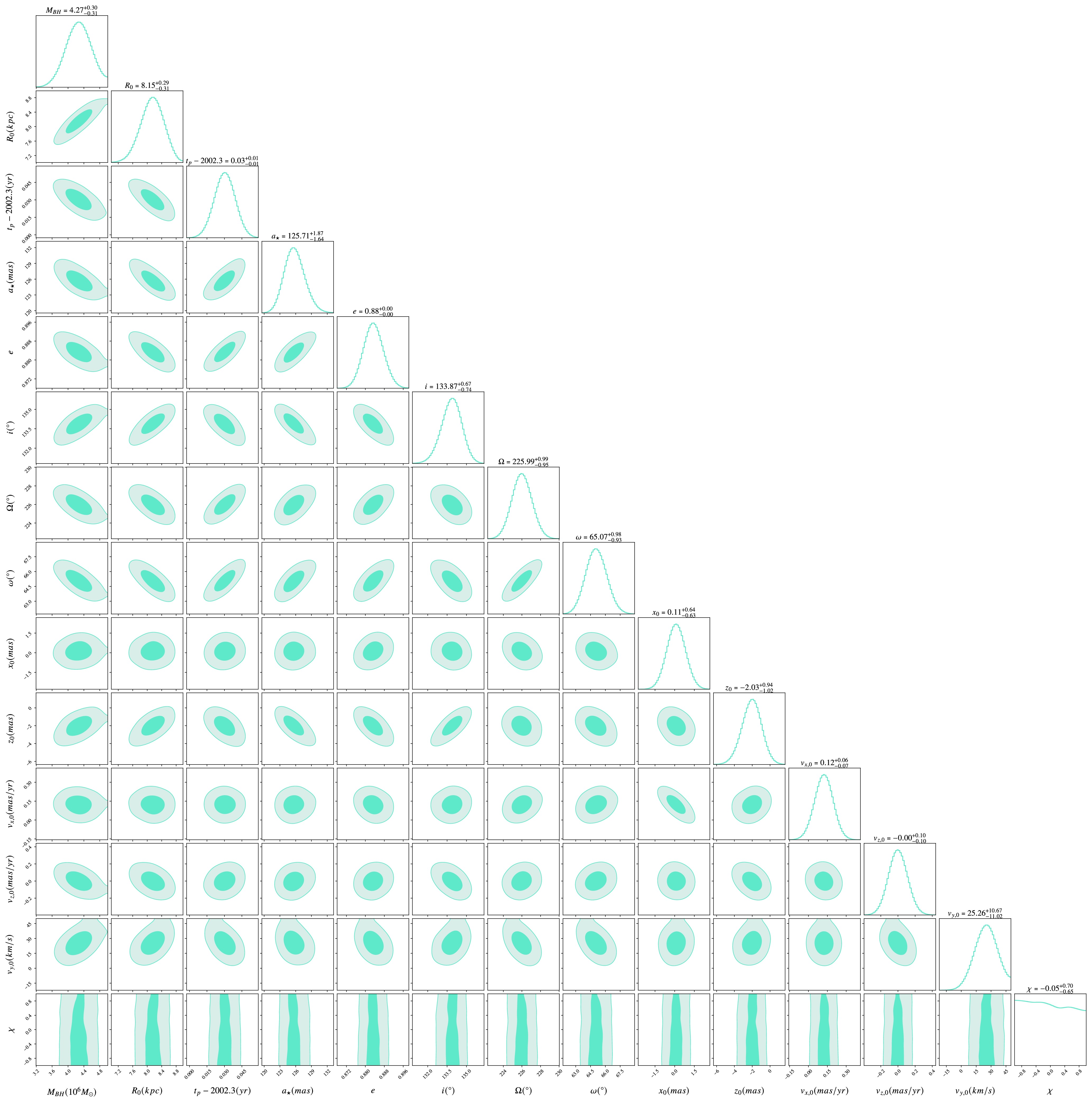

Figure 2.  (color online) The posterior distributions of the 14 parameters $ \left\{ M_{\rm BH},\chi,R_0,t_p,a_\star,e,i,\Omega,\omega,x_0,z_0,v_{x,0},v_{z,0},v_{y,0} \right\} $ in Kerr spacetime. For each pair of parameters, the 2D contour plots embracing (from darker to lighter) the 68% and 95% of the posterior samples in the off-diagonal plots. The marginalized 1D posterior distributions and corresponding $ 1\sigma $ range for each parameter are showed on the diagonal.

If stars are situated in close proximity to Sgr A$ ^\star $, even a shorter monitoring period could be sufficient to examine its spin behavior. However, we have not yet detected such stars. In order to clearly show the effects of spin on the orbit, we assume the presence of some such stars as probes. Meanwhile, we assume that these stars are stable. Based on the best-fit values of orbital elements on S2 star, as shown in column 3 of Table 1, we only change the semi-major axis and eccentricity to simulate these test stars. We simulate a total of 4 stars, whose inclination angle, longitude of the ascending node and argument of pericenter are consistent with S2, namely, $ i = 133.87 $, $ \Omega = 225.99 $ and $ \omega = 65.07 $. The semi-major axis and eccentricity of the simulated stars, labeled with the letter "T", are as follows: (T1) $ a_\star = 10 $ A.U. and $ e = 0.5 $, (T2) $ a_\star = 10 $ A.U. and $ e = 0.8 $, (T3) $ a_\star = 20 $ A.U. and $ e = 0.5 $, and (T4) $ a_\star = 20 $ A.U. and $ e = 0.8 $. Under these orbital elements, these four simulated stars all spin clockwise around the $ z $-axis. The orbital precession and Lense-Thirring precession on simulated stars orbiting different extreme Kerr black holes and Schwarzschild black hole are shown in Table 2. One can find that for same amplitude of spin, the influence on orbital effect for opposite spin are evident. When the orbital motion of simulated star is aligned with the spin direction, the orbital precession is smaller than when they are in opposite directions. Furthermore, changes in the direction of black hole spin will also induce changes in the direction of the Lense-Thirring precession. Interestingly, the direction of Lense-Thirring precession is consistent with the spin direction of the black hole. The drag of a black hole on spacetime originates from its spin, which causes the direction of motion of the orbital plane to change as the spin changes. These differences provide a window to determine the spin of Sgr A$ ^\star $.

Effect	Star	$ a_\star $(A.U.)	$ e $	$ i(^\circ) $	$ \Omega(^\circ) $	$ \omega(^\circ) $	$ \chi=-1 $	$ \chi=0 $	$ \chi=1 $
Orbital Precession	T1	10	0.5	133.87	225.99	65.07	5.78$ ^\circ $	6.16$ ^\circ $	6.48$ ^\circ $
	T2	10	0.8	133.87	225.99	65.07	11.67$ ^\circ $	12.83$ ^\circ $	13.81$ ^\circ $
	T3	20	0.5	133.87	225.99	65.07	2.94$ ^\circ $	3.06$ ^\circ $	3.17$ ^\circ $
	T4	20	0.8	133.87	225.99	65.07	6.03$ ^\circ $	6.37$ ^\circ $	6.71$ ^\circ $
Lense Thirring Precession	T1	10	0.5	133.87	225.99	65.07	-17.86$ ^\prime $	—–	18.99$ ^\prime $
	T2	10	0.8	133.87	225.99	65.07	-52.63$ ^\prime $	—–	57.58$ ^\prime $
	T3	20	0.5	133.87	225.99	65.07	-6.34$ ^\prime $	—–	6.61$ ^\prime $
	T4	20	0.8	133.87	225.99	65.07	-18.89$ ^\prime $	—–	20.11$ ^\prime $

Table 2.  Orbital precession and Lense-Thirring precession of simulated stars orbiting Sgr A$ ^\star $ with different spin. The mass of Sgr A$ ^\star $ is set as $ M_{\rm BH} = 4.27 \times 10^6 M_\odot $. Column 2: the ID of star, where "T" indicates a simulated star.; Column 3-4: the falsified semi-major axis and eccentricity of simulated star; Column 5-7: the orbital inclination angle, longitude of the ascending node and argument of pericenter of simulated star, which are the best fit values of S2 star come from Table 1; Column 8-10: the calculation results of orbital precession and Lense-Thirring precession with different extreme dimensionless spin.

As mentioned earlier, our universe is expanding, and observational data of S2 star provides a valuable tool for conducting this study. Following the methods mentioned earlier in this section, we investigate the Kerr-de Sitter spacetime. In the MCMC simulations here, the parameter space consists of Eq. (43), the dimensionless spin $ \chi $ of black hole and cosmological constant $ \Lambda $, for a total of 15 parameters.

Same as before, here we set a uniform prior, as shown in the column 2 of Table 1. The results of our Bayesian analysis are listed in column 4 of Table 1, where we show the best fit values and the corresponding $ 1\sigma $ ranges. For the same parameters, these result agrees with that of Kerr spacetime within the error range. The confidence regions and posterior distribution of the specific spacetime parameters $ \left\{ \chi, \Lambda \right\} $ we are interested in are shown in Figure 3. In the contour plot, we present the allowed region of interest (at $ 1\sigma $ and $ 2\sigma $ confidence level) for the parameters $ \chi $ and $ \Lambda $ derived from our analysis. The marginalized posterior distributions for these parameters are displayed on the diagonal of the corner plot. For the parameter $ \chi $, its posterior probability distribution is still smooth and approximates its uniform prior. For parameter $ \Lambda $, our orbital model for S2 tends to prefer a small value of $ \Lambda $, generally below $ 0.16\times10^{-13}{\rm A.U.}^{-2} $ $ (\approx 7.3\times10^{-34}{\rm km}^{-2}) $ at $ 1\sigma $ confidence level. Such an upper limit is far from the estimate from observational cosmological analysis. It should be emphasized that our results are based on local observations. The accuracy of the observational data for the S2 star is limited, and the dataset is relatively sparse. Long-term, high-precision observations of the abnormal average motion of Mercury in the solar system yielded $ 1\sigma $ upper bound on cosmological constant is about $ 1\times10^{-34}{\rm km}^{-2} $ [61], which is consistent with our results. Continued observations of S2 and other S-cluster stars in the future may improve the limitation on the cosmological constant by several orders of magnitude. This goal can also be achieved by improving the accuracy of observations.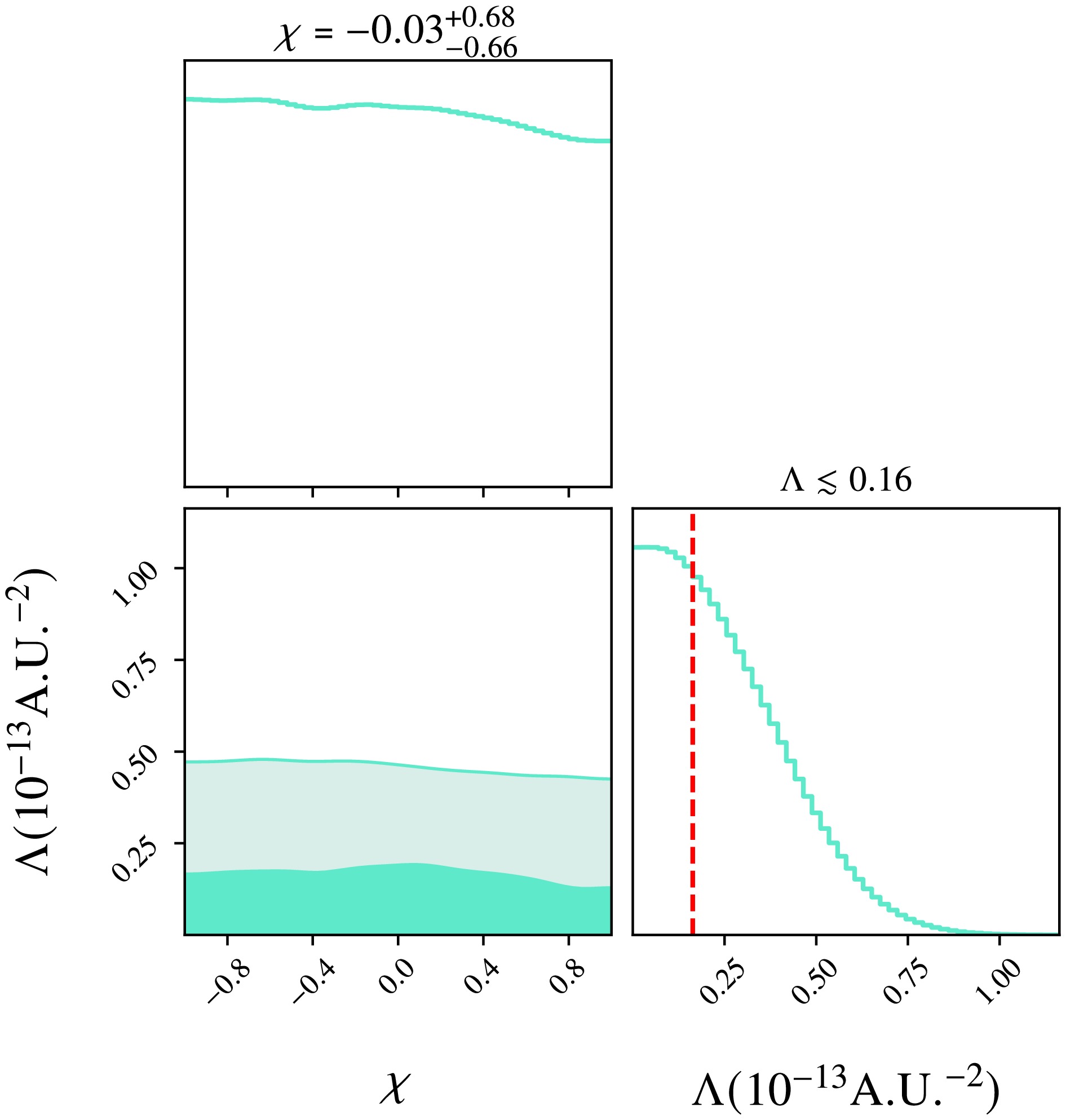

Figure 3.  (color online) The posterior distributions for the parameters mainly studied in our simulations, namely, $ \chi $ and $ \Lambda $. The red dashed lines, corresponding to the value of $ \Lambda \sim 0.16\times10^{-13}{\rm A.U.}^{-2} $, stand for the $ 1\sigma $ confidence level for cosmological constant in our analysis.

In this paper, we have investigated the dynamics of S2 star orbiting the supermassive black hole Sgr A$ ^\star $ at the center of the Milky Way. We primarily investigated the impact of the black hole spin on the orbit of the S2 star as it revolves around Sgr A$ ^\star $. In addition, we discussed the impact of the cosmological constant. Using publicly available astrometric and spectroscopic data of S2 star, we perform an MCMC bayesian analysis to place constraints on the black hole spin and the cosmological constant. The analysis results show that the observational data of S2 star fail to provide an effective and strong limit on the spin of Sgr A$ ^\star $. However, from the changing trend of the posterior probability distribution of the parameter $ \chi $, we can see that it tends to values less than zero, suggesting that Sagittarius A$ ^\star $ spins clockwise around the $ z $-axis. Furthermore, we simulated that some stars are in close proximity to Sgr A$ ^\star $ (with smaller semi-major axis). In the extreme case of black hole spin, we find that the influence of spin on orbital precession and Lense-Thirring precession is obvious and easy to observe. Specifically, the direction of Lense-Thirring precession aligns with the spin direction of the black hole. Additionally, we incorporated the cosmological constant, which accounts for the expansion of the universe, into our analysis. The results show that at the $ 1\sigma $ confidence level, the upper limits of the cosmological constant are set to $ \Lambda \lesssim 7.3 \times 10^{-34}{\rm km}^{-2} $. This limitation is consistent with the consequences within the solar system [61]. It is hoped that in the future we can use higher-precision and more observational data to obtain more precise results on the spin of Sgr A$ ^\star $ to uncover this mystery [20], and we also hope to obtain a more accurate cosmological constant in the region of strong gravitational fields.