


 Abstract
 HTML
HTML Reference
 Related
 PDF
PDF


-
The extreme-gravity regions of the universe, where black holes (BHs) and compact objects (COs) reside, are a treasure trove for testing the theory of gravity and exploring the secrets of spacetime. The detection of gravitational waves (GWs) [1−3] has opened new channels to probe these highly-dynamical, strong-curvature regions by observing binaries of BHs and COs [4−6]. The study of GW astrophysics inspires us with great confidence in fundamental theories and new physics [7, 8]. An important frequency window for GW detections is the extreme mass ratio inspiral (EMRI) [9]. During the inspirals of a stellar mass body (the secondary) orbiting a central supermassive BH (the primary), the EMRI system radiates tens to hundreds of thousands of GW cycles. The accumulated signal provides an effective tool to probe the near-horizon environment of BHs [10−13], source localization [14], massive BH spectrum, and corresponding evolution [15−17]. The space-based GW detectors that are currently under development, such as the Laser Interferometer Space Antenna (LISA) [18, 19], DECIGO [20], Taiji [21, 22], and TianQin [22, 23], will target EMRIs as their primary detection sources.
In general relativity (GR), binary systems emit GWs with tensor polarizations, and the lowest radiative multipole moment is the quadrupole moment. However, in alternative theories of gravity, additional emission channels may exist. For example, in Brans-Dicke theory and some scalar-tensor theories, the additional scalar field activates the dipole gravitational radiation reaction [24−27]. Even if these additional modes physically exist, the milli-Hz low frequency band GWs have significantly lower strength compared to the tensorial polarizations [28, 29], making them more difficult to observe by the planned space-borne missions. The long-time duration characteristics of an EMRI make it a competitive way to detect these additional modes. Typically, the entire process of the inspiral of the secondary in an EMRI lasts tens to hundreds of years. As a result, although the instantaneous strength of the additional radiation is less significant when compared with the tensor modes, the accumulated signal could possibly deviate from that determined by GR, with the dynamics of the EMRI systems modified by the presence of the additional radiation. In Ref. [30], the authors showed that, for specific classes of scalar-tensor alternative gravity theories, the EMRI could be considered as a test particle with a scalar charge inspiraling onto the central supermassive BH. They demonstrated that the corresponding dephasing caused by the scalar radiation should be detectable by LISA. This is an impressive model that offers twofold benefits. On the one hand, it allows studying the extra scalar radiation and how it differs from EMRI waveforms in GR, providing a way to test gravity theories in the strong field regime. The study reported in Ref. [31] investigated LISA's ability to detect the model-independent scalar charge and proposed a GW template for detecting new fundamental fields in our universe. The research has been extended to Kerr spacetime [32], eccentric equatorial orbits [33, 34], and the massive scalar field case [35]. Additionally, in Ref. [36], the extra radiation of the electromagnetic field was considered for the first time, and the detectability of the electromagnetic charge by EMRI GW signals from LISA was analyzed. Several recent studies have focused on this topic [37, 38]. On the other hand, the approach proposes an EMRI model that allows investigating the properties of binaries in this modified gravity. One particular property of interest is the effect of the secondary spin during inspirals, which has been extensively studied in EMRIs [39−41].
Many astrophysically relevant BHs or COs have nonzero angular momentum [42, 43], and to obtain a highly accurate theoretical waveform, it is reasonable to take into account the spin of the secondary in EMRIs [39, 44, 45]. Furthermore, precise detection of the secondary spin can help us study the properties of the secondary objects, which is an initial step in building a spectrum of stellar-mass to intermediate-BH-mass compact objects [15]. However, most studies on the effect of the secondary spin in EMRIs have been limited to GR (see recent works [46−50]), and it would be valuable to extend this research to modified gravity. First, the spin-curvature interaction will deviate the secondary from the geodesic motion in GR. Then, the secondary spin contributions may also arise from the additional radiation of the GW signal in the modified gravitational EMRI model. With these considerations, the extra scalar energy fluxes potentially enhance the secondary spin effect in GWs, resulting in the improvement of secondary spin detection by space-based GW detectors. Despite this potential, none of the previous studies related to the model in Ref. [30] computed the spin-correction of the secondary to the GW phase. It is interesting to focus our attention on this topic.
In the present study, our objective is to extend the model proposed in Ref. [30] to study the detection of spin-corrections of the secondary. The spin-curvature coupling, described by the MPD equations, is the leading order effect of the finite size of a rapidly rotating compact astrophysical object moving in a curved background. It is a next-to-leading order effect in the phase of GWs emitted by EMRIs and is expected to be comparable to the effect induced by the additional scalar radiation. Therefore, as one aims to detect the scalar charge by studying the additional scalar radiation, it is reasonable to expect secondary spin detection with the additional scalar radiation. In this EMRI model, we calculate the related GW fluxes and GW phases and compare the detectability of LISA, Taiji, and TianQin using the parameter estimation approaches. The results demonstrate that the presence of the scalar field amplifies the secondary spin effect, allowing for the detection of a lower limit value of the secondary spin and an improved resolution of secondary spin detection when the scalar charge is sufficiently large.
The rest of this paper is organized as follows. Sec. II describes the construction of the EMRI system and introduces the orbit motion of the spinning test particle in the Kerr spacetime. Sec. III presents the tensor perturbation and scalar perturbation, and the energy fluxes are obtained by solving the perturbation equations. In Sec. IV, we discuss the orbital evolution, total energy fluxes, dephasing, and related faithfulness of the GW signals. Finally, we summarize our results and present concluding remarks in Sec. V. Throughout the paper, we use geometric units as
$ c=G=1. $ -
Recent research has revealed that, in a broad range of gravity theories involving scalar fields with non-minimal coupling, the scalar charge of the secondary object can significantly influence the emission observed in EMRIs [30−33]. This influence is expected to be detectable with the future space-based GW projects such as LISA, Taiji, and TianQin. Using an effective field theory approach, it has been observed in some types of modified gravity theories when the scalar charge of the primary object can be considered negligible at the leading order, whereas the charge of the secondary remains finite. Consequently, this simplifies the treatment of EMRIs beyond GR, allowing the primary object to be effectively described by the Kerr metric, whereas any deviations from GR are primarily determined by the scalar charge of the secondary object. With this consideration, we examine the case of a spinning secondary spiraling into a central supermassive Kerr BH with the inclusion of a scalar field coupling to higher-order curvature instants during the quasi-circular orbital evolution in the equatorial plane. We begin by outlining the model framework and then provide a brief overview of the orbital motion of the spinning particle.
-
We consider the EMRIs described by the action [30]
$\begin{aligned}[b] S[g_{\mu\nu},\phi,\Psi]=\;&S_0[g_{\mu\nu},\phi]+\alpha S_c[g_{\mu\nu},\phi]\\&+S_m[g_{\mu\nu},\phi,\Psi],\end{aligned} $

(1) with
$ S_0=\int d^4x \frac{\sqrt{-g}}{16\pi}\left(R-\frac{1}{2}\partial_{\mu}\phi\partial^{\mu}\phi\right), $

(2) where R is the Ricci scalar.
$ S_c $ describes the nonminimal coupling between the scalar field$ \phi $ and the metric tensor, and$ \alpha $ is the coupling parameter with dimensions$ [\alpha]=(mass)^n $ . The matter field action$ S_m[g_{\mu\nu},\phi,\Psi] $ describes the spinning secondary. Varying the action in Eq. (1), one obtains the equations of motion$ G_{\mu \nu}=R_{\mu \nu}-\frac{1}{2} g_{\mu \nu} R=T_{\mu \nu}^{\text{scal}}+\alpha T_{\mu \nu}^{c}+T_{\mu \nu}^{p}, $

(3) $ \square \phi+\frac{16 \pi \alpha}{\sqrt{-g}} \frac{\delta S_{c}}{\delta \phi}=16 \pi\ {\cal{T}}_{\rm scalar} , $

(4) where
$ T_{\mu \nu}^{\text{scal}}=\dfrac{1}{2} \partial_{\mu} \phi \partial_{\nu} \phi-\dfrac{1}{4} g_{\mu \nu}(\partial \phi)^{2} $ is the stress-energy tensor of the scalar field,$ \alpha T_{\mu \nu}^{c} $ is the stress-energy of the coupling term, and$ T_{\mu\nu}^p $ represents the stress-energy tensor of the spinning secondary.${\cal{T}}_{\rm scalar}$ is the source term, which is obtained by varying$ S_m $ with respect to$ \phi $ .By using the skeletonization approximation, the scalar field can be approximated to
$\phi=\phi_0+{m_p d}/{r}+...$ far away from the matter source, where$ \phi_0 $ represents the background value of the scalar field, d denotes the dimensionless scalar charge of the test body, and$ m_p $ is the mass of the secondary. Note that the scalar field in spacetime is directly coupled to the geometry, and the interaction between the scalar field and the secondary is reflected by a mass function$ m(\phi) $ . After simplification, it is convenient to obtain the relation$ m(\phi_0)=m_p $ and$m^{\prime}(\phi_0)/ m(\phi_0) = -d/4$ .Therefore, the gravitational perturbation is described by a spinning secondary with mass
$ m(\phi_0)=m_p $ spiraling into a supermassive Kerr BH. Following the discussion in [47], the stress-energy tensor$ T_{\mu\nu}^p $ reduces to the stress-energy tensor of a spinning test particle$\begin{aligned}[b] T_{\mu\nu}^p=\;&8\pi\,m_{p}\int {\rm{d}} \lambda\left[\frac{\delta^{(4)}\left(x-y_{p}(\lambda)\right)}{\sqrt{-g}} u^{(\mu} v^{\nu)}\right.\\&\left.-\nabla_{\sigma}\left(S^{\sigma(\mu} v^{\nu)} \frac{\delta^{(4)}\left(x-y_{p}(\lambda)\right)}{\sqrt{-g}}\right)\right].\end{aligned} $

(5) As we neglect the directive interaction between the scalar field and the secondary spin, which is a higher-order infinitesimal interaction in this model, the scalar perturbation is sourced by the trajectory motion of the spinning secondary. Consequently, considering the result mentioned in [30, 32], the source term of the scalar field reduces to
$ {\cal{T}}_{\rm scalar}=-\frac{d}{4}m_p\int\frac{{\rm d} t}{v^t} \frac{\delta^{(4)}\left(x-y_{p}(t)\right)}{\sqrt{-g}}. $

(6) As a result, the equations of motion can be expressed as
$\begin{aligned}[b] G_{\mu\nu}=\;&T^{\rm p}_{\mu\nu}=8\pi\, m_{p}\int {\rm{d}} \lambda\left[\frac{\delta^{(4)}\left(x-y_{p}(\lambda)\right)}{\sqrt{-g}} u^{(\mu} v^{\nu)}\right.\\&\left.-\nabla_{\sigma}\left(S^{\sigma(\mu} v^{\nu)} \frac{\delta^{(4)}\left(x-y_{p}(\lambda)\right)}{\sqrt{-g}}\right)\right] ,\end{aligned} $

(7) $ \square\phi=-4\pi d\,m_{\rm p}\int\frac{{\rm d} t}{v^t} \frac{\delta^{(4)}(x-y_{\rm p}(t))}{\sqrt{-g}}\,. $

(8) where
$ y_p $ is the worldline of the secondary, and$ \lambda $ is the affine parameter, which is set as the proper time. The 4-velocity and normalized momenta of the secondary are represented by$ v^\mu $ and$ u^\mu $ , respectively. Additionally, we use a skew-symmetric tensor$ S^{\mu\nu} $ to derive the spin parameter, which can be obtained using$ S^{2} \equiv \frac{1}{2} S^{\mu \nu} S_{\mu \nu} $ . To simplify our discussion, we introduce the reduced spin parameter$ \chi=\sigma/q $ , where$ \sigma=S/(m_p M) $ is the related dimensionless spin parameter and the mass ratio is$ q=m_p/M $ . For a more detailed discussion of the spinning orbital evolution, please refer to subsection II.B.In this study, we investigate a spinning secondary adiabatically spiraling into the central supermassive Kerr BH with a quasi-circular orbital evolution in the equatorial plane. The background Kerr metric reads
$\begin{aligned}[b] {\rm d} s^{2}=\;&-\left(1-\frac{2 M r}{\Sigma}\right) {\rm d} t^{2}+\frac{\Sigma}{\Delta} {\rm d} r^{2}-\frac{4 M a r \sin ^{2} \theta}{\Sigma} {\rm d} t {\rm d} \varphi\\&+\Sigma {\rm d} \theta^{2}+\frac{\sin ^{2} \theta}{\Sigma}\left(\varpi^{4}-a^{2} \Delta \sin ^{2} \theta\right) {\rm d} \varphi^{2},\end{aligned} $

(9) where
$\Sigma \equiv r^{2}+a^{2} \cos ^{2} \theta,~ \Delta \equiv r^{2}-2 M r+a^{2}, ~ \varpi \equiv \sqrt{r^{2}+a^{2}}$ . M and a are the mass and spin of the Kerr BH, respectively. Here, we introduce the dimensionless parameters as$\hat{a}=a/M,~ \hat{t}=t/M,~ \hat{r}=r/M$ , and thus, we have$\{\hat{\Sigma},\hat{\Delta}, \hat{\varpi}\}= \{\Sigma, \Delta, \varpi\}/M^2$ . The inner and outer horizons are given by$ \hat{r}_{\pm}=1\pm\sqrt{1-\hat{a}^2} $ , and the tortoise coordinate is defined by${\rm d} \hat{r}/\hat{r}_*=\hat{\Delta}/(\hat{r}^2+\hat{a}^2)$ . -
In this EMRI system, the size of the secondary is significantly smaller than that of the central BH; therefore, its stress-energy tensor
$ T_{\mu\nu} $ can be approximated by a multipolar expansion within gravitational skeletonization. Treating the secondary as a spinning particle corresponds to retaining only the first two multipoles. The covariant conservation of the energy-momentum tensor results in the Mathisson-Papapetrou-Dixon (MPD) equations [47]$ \begin{aligned}[b] {\frac{{\rm{d}} y_p^{\mu}}{{\rm{d}} \lambda}} &{=v^{\mu}}, \\ {\nabla_{\vec{v}} p^{\mu}} &{=-\frac{1}{2} R_{\nu \alpha \beta}^{\mu} v^{\nu} S^{\alpha \beta}}, \\ {\nabla_{\vec{v}} S^{\mu \nu}} &{=2 p^{[\mu} v^{\nu]}}, \\ {\mathfrak{m}} & {\equiv-p_{\mu} v^{\mu}}, \end{aligned} $

(10) where the 4-velocity
$ v^\mu $ is defined by the worldline$ y_p^\mu(\lambda) $ , and$ \nabla_{\vec{v}} \equiv v^{\mu} \nabla_{\mu} $ . The spin parameter S is defined by the skew-symmetric tensor as$S^{2} \equiv S^{\mu \nu} S_{\mu \nu}/2$ , and the linear momentum and 4-velocity are not aligned with$p^{\mu}= {v^{-2}}\left(\mathfrak{m} v^{\mu}-v_{\sigma} \nabla_{\vec{v}} S^{\mu \sigma}\right)$ because$ \mathfrak{m} $ represents the monopole rest-mass. Here, we introduce the dynamical rest mass of the point particle as$ m_p^2=-p^\sigma p_\sigma $ . Thus, the normalized momenta is given by$ u^\mu=p^\mu/m_p $ , which satisfies$ u^\mu u_\mu=-1 $ .We take the spin-supplementary condition by the Tulczyjew-Dixon equation
$ S^{\mu \nu} p_{\nu}=0. $

(11) By incorporating the Kerr metric into these equations, the MPD equations can be expressed as exact formulas in Boyer-Lindquist coordinates:
$ \Sigma_{\sigma} \Lambda_{\sigma} \frac{{\rm{d}} \hat{t}}{{\rm{\; d}} \hat{\lambda}}=\hat{a}\left(1+\frac{3 \sigma^{2}}{\hat{r} \Sigma_{\sigma}}\right)\left[\hat{J}_{z}-\hat{E}(\hat{a}+\sigma)\right]+\frac{\hat{r}^{2}+\hat{a}^{2}}{\hat{\Delta}} P_{\sigma} $

(12) $ \left(\Sigma_{\sigma} \Lambda_{\sigma}\right)^{2}\left(\frac{{\rm{d}} \hat{r}}{{\rm{\; d}} \hat{\lambda}}\right)^{2}=R_{\sigma}^{2}$

(13) $ \Sigma_{\sigma} \Lambda_{\sigma} \frac{{\rm{d}} \phi}{{\rm{d}} \hat{\lambda}}=\left(1+\frac{3 \sigma^{2}}{\hat{r} \Sigma_{\sigma}}\right)\left[\hat{J}_{z}-\hat{E}(\hat{a}+\sigma)\right]+\frac{\hat{a}}{\hat{\Delta}} P_{\sigma} $

(14) with
$ \begin{aligned}[b] \Lambda_{\sigma}=\;&1-\dfrac{3 \sigma^{2} \hat{r}\left[-(\hat{a}+\sigma) \hat{E}+\hat{J}_{z}\right]^{2}}{\Sigma_{\sigma}^{3}} \\ R_{\sigma}=\;&P_{\sigma}^{2}-\hat{\Delta}\left(\dfrac{\Sigma_{\sigma}^{2}}{\hat{r}^{2}}+\left[-(\hat{a}+\sigma) \hat{E}+\hat{J}_{z}\right]^{2}\right) \\ P_{\sigma}=\;&\left[\left(\hat{r}^{2}+\hat{a}^{2}\right)+\dfrac{\hat{a} \sigma}{\hat{r}}(\hat{r}+1)\right] \hat{E}-\left[\hat{a}+\dfrac{\sigma}{\hat{r}}\right] \hat{J}_{z}, \end{aligned} $

(15) where
$ \Sigma_{\sigma}=\hat{r}^{2}\left(1-\dfrac{\sigma^{2}}{\hat{r}^{3}}\right)>0 $ . It is convenient to demonstrate that the geodesic equations given by Eqs. (12)−(14) reduce to nonspinning geodesic motion when$ \sigma\rightarrow 0 $ . In this EMRI model, we focus on the circular orbital motion on the equatorial plane, which implies that both the radial velocity and radial acceleration are zero. The details of the calculation are omitted here but can be found in [47]. After simplification, we can determine the orbital frequency as measured by a static observer located at infinity:$ \hat{\Omega}=M\Omega=\frac{(2 \hat{a}+3 \sigma) \hat{r}^{3}+3\left(2 \hat{a}^{2} \sigma+\hat{a} \sigma^{2}\right) \hat{r}+4 \hat{a} \sigma^{2} \mp \hat{r} {\cal{D}}}{2\left(\hat{a}^{2}+3 \hat{a} \sigma+\sigma^{2}\right) \hat{r}^{3}+6 \sigma(\hat{a}+\sigma) \hat{a}^{2} \hat{r}+4 \hat{a}^{2} \sigma^{2}-2 \hat{r}^{6}}, $

(16) where
$ {\cal{D}}=\sqrt{4 \hat{r}^{7}+12 \hat{a} \sigma \hat{r}^{5}+13 \sigma^{2} \hat{r}^{4}+6 \hat{a} \sigma^{3} \hat{r}^{2}-8 \sigma^{4} \hat{r}+9 \hat{a}^{2} \sigma^{4}}. $

(17) The first integrals of the spinning particle's motion, which are the orbital energy
$ \hat{E} $ and orbital angular momentum$ \hat{J}_z $ , can be expressed by$ \hat{E} =\frac{E}{M}=\frac{\hat{r} \sqrt{\hat{\Delta}}+(\hat{a} \hat{r}+\sigma) U_{\mp}}{\hat{r}^{2} \sqrt{1-U_{\mp}^{2}}} , $

(18) $ \hat{J}_{z} =\frac{J_z}{m_pM}=\frac{\hat{r} \sqrt{\hat{\Delta}}(\hat{a}+\sigma)+\left[\hat{r}^{3}+\hat{r} \hat{a}(\hat{a}+\sigma)+\hat{a} \sigma\right] U_{\mp}}{\hat{r}^{2} \sqrt{1-U_{\mp}^{2}}} , $

(19) with
$ U_{\mp}=-\frac{2 \hat{a} \hat{r}^{3}+3 \sigma \hat{r}^{2}+\hat{a} \sigma^{2} \mp {\cal{D}}}{2 \sqrt{\hat{\Delta}}\left(\hat{r}^{3}+2 \sigma^{2}\right)}, $

(20) where the sign
$ \mp $ represents prograde and retrograde orbits, respectively. The expressions of the conserved quantities (18) and (19), as well as the orbital frequency (16), will be useful when studying the adiabatic evolution of the spinning orbital motion. -
The wave equation of the metric perturbation can be obtained by the Teukolsky formalism, which is governed by the
$ \psi_4 $ Weyl scalar:$ \psi_{4}=\rho^{4} \sum\limits_{\ell=2}^{\infty} \sum\limits_{m=-\ell}^{\ell} \int_{-\infty}^{\infty} {\rm d} \hat{\omega} R_{\ell m \hat{\omega}}(\hat{r})_{-2} S_{\ell m}^{\hat{a} \hat{\omega}}(\theta) {\rm e}^{{\rm i} (m \varphi-\hat{\omega} \hat{t})}, $

(21) where
$\rho=(\hat{r}- {\rm i} \hat{a}\cos\theta)^{-1}$ . The$ s=-2 $ spin weighted orthonormal spheroidal harmonics is$ _{-2} S_{\ell m}^{\hat{a} \hat{\omega}} $ with its eigenvalue$ \lambda_G $ . At infinity, the GW polarizations are given by the relation$ \psi_4=\frac{1}{2}\frac{\partial^2}{\partial \hat{t}^2}(h_+- {\rm i} h_\times). $

(22) The radial Teukolsky equation is
$ \hat{\Delta}^{2} \frac{\rm d}{{\rm d} \hat{r}}\left(\frac{1}{\hat{\Delta}} \frac{{\rm d} R_{\ell m \omega}(\hat{r})}{{\rm d} \hat{r}}\right)-V_G(\hat{r}) R_{\ell m \hat{\omega}}(\hat{r})={\cal{T}}^T_{\ell m \hat{\omega}}, $

(23) with its effective potential
$ V_G(\hat{r})=-\frac{K^{2}+4 {\rm i} (\hat{r}-1) K}{\hat{\Delta}}+8 {\rm i} \hat{\omega} \hat{r}+\lambda_G, $

(24) where
$ K=\left(\hat{r}^{2}+\hat{a}^{2}\right) \hat{\omega}-\hat{a} m $ . The homogeneous Teukolsky equation has two linearly independent solutions that satisfy pure ingoing boundary conditions near horizon$ R_{\ell m\hat{\omega}}^{\rm in} $ and pure outgoing boundary conditions at infinity$ R_{\ell m\hat{\omega}}^{\rm out} $ . Through the Green's function method, the solution of the inhomogeneous Teukolsky equation is obtained by$\begin{aligned}[b] R_{\ell m \hat{\omega}}(\hat{r}) =\;&\frac{1}{W_{G }}\left\{R_{\ell m \hat{\omega}}^{\rm{out}}(\hat{r}) \int_{\hat{r}_+}^{\hat{r}} {\rm{\; d}} \hat{r}^{\prime} \frac{R_{\ell m \hat{\omega}}^{\rm{in}}\left(\hat{r}^{\prime}\right) {\cal{T}}^{T}_{\ell m \hat{\omega}}\left(\hat{r}^{\prime}\right)}{\hat{\Delta}^{2}}\right.\\&\left.+R_{\ell m \hat{\omega}}^{\rm{in}}(\hat{r}) \int_{\hat{r}}^{\infty} {\rm{d}} \hat{r}^{\prime} \frac{R_{\ell m \hat{\omega}}^{\rm{out}}\left(\hat{r}^{\prime}\right) {\cal{T}}^{T}_{\ell m \hat{\omega}}\left(\hat{r}^{\prime}\right)}{\hat{\Delta}^{2}}\right\}, \end{aligned}$

(25) with the constant Wronskian
$W_G\equiv R^{\rm in}_{\ell m\hat{\omega}}{\rm d}R^{\rm out}_{\ell m\hat{\omega}}/{\rm d}\hat{r}_*- R^{\rm out}_{\ell m\hat{\omega}}{\rm d}R^{\rm in}_{\ell m\hat{\omega}}/{\rm d}\hat{r}_*$ . The source term$ {\cal{T}}^T_{\ell m \hat{\omega}} $ is obtained by the stress-energy tensor in Eq. (7) by the Newman-Penrose formalism; further details can be found in [47, 51].The solution of the inhomogeneous Teukolsky equation also satisfies pure ingoing boundary conditions near the horizon and pure outgoing boundary conditions at infinity
$ \begin{aligned}[b] R_{\ell m \hat{\omega}}\left(\hat{r} \rightarrow \hat{r}_+\right) =\;&Z_{\ell m \hat{\omega}}^{\infty} \hat{\Delta}^{2} {\rm e}^{-{\rm i} \hat{\kappa} \hat{r}_{*}}, \\ R_{\ell m \hat{\omega}}(\hat{r} \rightarrow \infty) =\;&Z_{\ell m \hat{\omega}}^{H} \hat{r}^{3} {\rm e}^{{\rm i} \hat{\omega} \hat{r}_{*}}, \end{aligned} $

(26) with the coefficients
$ \begin{aligned}[b]Z_{\ell m \hat{\omega}}^{\infty}=\;&C_{\ell m \hat{\omega}}^{\infty} \int_{\hat{r}_+}^{\infty} {\rm{d}} \hat{r}^{\prime} \frac{R_{\ell m \hat{\omega}}^{\rm{out}}\left(\hat{r}^{\prime}\right)}{\hat{\Delta}^{2}} {\cal{T}}^{T}_{\ell m \hat{\omega}}\left(\hat{r}^{\prime}\right), \\ Z_{\ell m \hat{\omega}}^{H}=\;&C_{\ell m \hat{\omega}}^{H} \int_{\hat{r}_+}^{\infty} {\rm{d}} \hat{r}^{\prime} \frac{R_{\ell m \hat{\omega}}^{\rm{in}}\left(\hat{r}^{\prime}\right)}{\hat{\Delta}^{2}} {\cal{T}}^{T}_{\ell m \hat{\omega}}\left(\hat{r}^{\prime}\right), \end{aligned} $

(27) where
$ C_{\ell m \hat{\omega}}^{H,\infty} $ can be found by Eq. (86) in [47]. For simplicity,$ \varphi(\hat{t})=\hat{\Omega} \hat{t} $ with a equatorial circular orbit, and we have$ Z_{\ell m \hat{\omega}}^{H, \infty}=\delta(\hat{\omega}-m \hat{\Omega}) {\cal{A}}_{\ell m \hat{\omega}}^{H, \infty}. $

(28) The scalar perturbation is expanded by the scalar spheroidal harmonics
$ \phi(\hat{t}, \hat{r}, \theta, \varphi)=\sum\limits_{\ell, m} \int {\rm d} \hat{\omega}\; {\rm e}^{{\rm i}(m \varphi-\hat{\omega}\hat{t})}\frac{X_{\ell m\hat{\omega}}(r)}{\sqrt{\hat{r}^{2}+\hat{a}^{2}}} {}_0 S_{\ell m}(\theta), $

(29) and the
$ s=0 $ orthonormal spheroidal harmonics is$ {}_0 S_{\ell m}(\theta) $ with the eigenvalue$ \lambda_s $ . Here, we write the radial scalar perturbation equation,$ \left[\frac{{\rm d}^{2}}{{\rm d} \hat{r}_{*}^{2}}+V_{s}(\hat{r})\right] X_{\ell m \hat{\omega}}(\hat{r})=\frac{\hat{\Delta}}{\left(\hat{r}^{2}+\hat{a}^{2}\right)^{3 / 2}} {\cal{T}}^s_{\ell m \hat{\omega}}, $

(30) with its effective potential
$ V_{s}=\left(\hat{\omega}-\frac{\hat{a} m}{\vartheta}\right)^{2}-\frac{\hat{\Delta}}{\vartheta^{4}}\left[\lambda_s \; \vartheta^{2}+2 \hat{r}^{3}+\hat{a}^{2}\left(\hat{r}^{2}-4 \hat{r}+\hat{a}^{2}\right)\right], $

(31) where
$ \vartheta=\hat{r}^2+\hat{a}^2 $ , and$ {\cal{T}}^s_{\ell m\hat{\omega}} $ is constructed from the source term on the right-hand side of Eq. (8). Similar to the case of gravitational perturbations, the homogeneous scalar perturbation equation has two linearly independent solutions, namely,$X_{\ell m\hat{\omega}}^{\rm in,out}$ , that satisfy pure ingoing boundary conditions near the horizon and pure outgoing boundary conditions at infinity. Using the Green's function method, the solution of the inhomogeneous equation can be constructed by$\begin{aligned}[b] X_{\ell m \hat{\omega}}(\hat{r}) =\;&X_{\ell m \hat{\omega}}^{\rm out}(\hat{r}) \int_{\hat{r}_+}^{\hat{r}} \; {\rm d} r^{\prime} \frac{X_{\ell m \hat{\omega}}^{\rm in}\left(r^{\prime}\right) {\cal{T}}^s_{\ell m \hat{\omega}}\left(r^{\prime}\right)}{W_{s}}\\&+X_{\ell m \hat{\omega}}^{\rm in}(\hat{r}) \int_{\hat{r}}^{\infty} {\rm d} r^{\prime} \frac{X_{\ell m \hat{\omega}}^{\rm out}\left(r^{\prime}\right) {\cal{T}}^s_{\ell m \hat{\omega}}\left(r^{\prime}\right)}{W_{s}}. \end{aligned}$

(32) Likewise, the constant Wronskian is
$W_s\equiv X^{\rm in}_{\ell m\hat{\omega}}{\rm d}X^{\rm out}_{\ell m\hat{\omega}}/{\rm d}\hat{r}_*- X^{\rm out}_{\ell m\hat{\omega}}{\rm d}X^{\rm in}_{\ell m\hat{\omega}}/{\rm d}\hat{r}_*$ . The inhomogeneous solution of the scalar perturbation can also give the boundary condition so that$ X_{\ell m \hat{\omega}}\left(\hat{r} \rightarrow \hat{r}_+\right) ={\cal{Z}}_{\ell m \hat{\omega}}^{\infty} {\rm e}^{-{\rm i} \hat{\kappa} \hat{r}_{*}}, $

(33) $ X_{\ell m \hat{\omega}}(\hat{r} \rightarrow \infty) ={\cal{Z}}_{\ell m \hat{\omega}}^{H} {\rm e}^{{\rm i} \hat{\omega} \hat{r}_{*}}, $

(34) with the coefficients
$ {\cal{Z}}_{\ell m \hat{\omega}}^{H, \infty}=-4\pi dq\frac{X_{\ell m \hat{\omega}}^{\rm in,up}\left(\hat{r}_{\rm p}\right)}{W_s\ u^{t}}\ \frac{{}_0 S_{\ell m}^{*}(\pi / 2)}{\sqrt{\hat{r}_{\rm p}^{2}+\hat{a}^{2}}}, $

(35) where
$ {}_0S_{\ell m}(\theta)^* $ is its complex conjugation and$\hat{\kappa}= m\hat{\Omega}- m\hat{a}/(2\hat{r}_+)$ .After we obtain the solution for both the gravitational perturbation and scalar perturbation, we can compute the energy fluxes of this model [52, 53]. From the gravitational perturbation part, the energy fluxes at the horizon and at infinity are
$ \dot{E}_{T}^{H}=\sum\limits_{\ell=2}^{\infty} \sum\limits_{m=1}^{\ell} \alpha_{\ell m} \frac{\left|{\cal{A}}_{\ell m \hat{\omega}}^{\infty}\right|^{2}}{2\pi(m \hat{\Omega})^{2}}, $

(36) $\dot{E}_{T}^{\infty}=\sum\limits_{\ell=2}^{\infty} \sum\limits_{m=1}^{\ell} \frac{\left|{\cal{A}}_{\ell m \hat{\omega}}^{H}\right|^{2}}{2\pi(m \hat{\Omega})^{2}}, $

(37) with the coefficients
$ \alpha_{\ell m}=\frac{256\left(2 \hat{r}_+\right)^{5} \hat{\kappa}\left(\hat{\kappa}^{2}+4 \epsilon^{2}\right)\left(\hat{\kappa}^{2}+16 \epsilon^{2}\right)(m \hat{\Omega})^{3}}{\left|C_{\ell m}\right|^{2}}, $

(38) $ \begin{aligned}[b]\left|C_{\ell m}\right|^{2}=\;&\left[\left(\lambda_G+2\right)^{2}+4 \hat{a}(m \hat{\Omega})-4 \hat{a}^{2}(m \hat{\Omega})^{2}\right]\\&\times\left[\lambda_G^{2}+36 m \hat{a}(m\hat{\Omega})-36\hat{a}^{2}(m \hat{\Omega})^{2}\right]\end{aligned} $

(39) $\begin{aligned}[b]\quad\quad&+\left(2 \lambda_G+3\right)\left[96 \hat{a}^{2}(m \hat{\Omega})^{2}-48 m \hat{a}(m \hat{\Omega})\right]\\&+144(m \hat{\Omega})^{2}\left(1-\hat{a}^{2}\right),\end{aligned} $

(40) where
$ \epsilon=\sqrt{1-\hat{a}^2}/(4\hat{r}_+) $ . From the scalar perturbation part, the energy fluxes are$ \dot{E}_{s}^{H}=\frac{1}{16\pi}\sum\limits_{\ell=1}^{\infty} \sum\limits_{m=-\ell}^{\ell} m \; \hat{\Omega} \; \hat{\kappa}\left|{\cal{Z}}_{l m \omega}^{\infty}\right|^{2},$

(41) $ \dot{E}_{s}^{\infty}=\frac{1}{16\pi}\sum\limits_{\ell=1}^{\infty} \sum\limits_{m=-\ell}^{\ell} m^2 \; \hat{\Omega}^2\left|{\cal{Z}}_{\ell m \omega}^{H}\right|^{2}. $

(42) By utilizing the code from the Black Hole Perturbation Toolkit [47, 54], we can numerically solve these perturbation equations. The total energy fluxes of the EMRI system are obtained from the numerical solutions
$ {\cal{F}}_{\rm tot}=\dot{E}_{T}+\delta\dot{E}_{s}=\dot{E}^H_T+\dot{E}^\infty_T+\delta\dot{E}^H_s+\delta\dot{E}^\infty_s, $

(43) where the subscript ''T'' stands for tensor modes, and the subscript ''s'' represents scalar modes. The superscripts ''H'' and ''
$ \infty $ '' refer to horizon and infinity, respectively.$ \dot{E}_T $ and$ \delta\dot{E}_s $ are the total gravitational energy flux and total scalar energy flux, respectively.Using the calculated total energy fluxes, we can now determine the adiabatic evolution of the spinning secondary, which is balanced by energy emissions:
$ \frac{{\rm d} r}{{\rm d}t}=-{\cal{F}}_{\rm tot}(t)\left(\frac{{\rm d} E}{{\rm d}r}\right)^{-1}\, , \frac{{\rm d}\varphi}{{\rm d}t}=\Omega(r(t)). $

(44) Here, orbital energy E is given by Eq. (18), and orbital frequency
$ \Omega $ is obtained from Eq. (16).$ \varphi $ represents the orbital phase, and for the dominant mode, the GW phase is given by$N_{\chi}^d=\varphi_{\rm GW}(t_{\rm end})=2\varphi(t_{\rm end})$ , where$ t_{\rm end} $ denotes the exit time when the evolution ends. -
In the following numerical calculations, we set the parameters as follows: without loss of generality, the primary spin is
$ a=0.9M $ , the primary mass is$ M=4\times 10^5M_{\odot} $ , and the secondary mass is$ m_p=10M_{\odot} $ . Thus, the mass ratio is$ q=2.5\times 10^{-5} $ . In the parameter space, we calculate the secondary spin in the range$ \chi\in[0,0.5] $ and the scalar charge in the range$ d\in[0,0.5] $ , while maintaining generality. All the multipole contributions are summed up to$ \ell=18 $ .Different from the original approach of simulating a one-year orbital evolution before plunging into ISCO, we adopt the modified approach commonly used in detecting the secondary spin [46−50]. In our approach, the spinning secondary starts at
$ r_{\rm start}=11.53M $ and spirals inwards the central BH. After evolution of one year, the simulation is terminated near$ r_{\rm ISCO} $ . Although our simulation ensures that the position of the secondary after one-year evolution is as close as possible to the ISCO, the accumulated phase obtained from our calculation will still be smaller than that of the original approach. However, we add an extra constraint on the initial position of the simulation, which greatly improves the results of the dephasing, enhancing the detection of GWs.For instance, we can contrast the amount of dephasing resulting from two distinct simulation methods. One approach involves a year-long orbital evolution followed by a plunge into the ISCO, whereas the other approach involves starting from the same initial position and undergoing a year-long evolution. We define
$ N_{\chi}^d $ as the total GW phase of our model, so$ N_{\chi=0}^d $ and$ N^{d=0}_{\chi} $ are the GW phases caused by the scalar charge and secondary spin, respectively, and$ N^{d=0}_{\chi=0} $ is the pure GR GW phase. In Appendix A, we present the data of dephasing$ |N_{\chi}^d-N_{\chi=0}^d| $ , describing the dephasing caused by the secondary spin. Table 1 presents the data simulated by our modified approach, whereas Table 2 summarizes the results obtained using the original approach. The first column contains the data in GR, and the subsequent columns show the results in modified gravity with scalar charge d. The modified approach exhibits significant advantages over the original approach. It can obtain a larger dephasing than the original approach for each parameter. Even in the GR case, the modified approach improves the dephasing to a larger extent than the original approach. It also shows a larger increase in dephasing for each secondary spin$ \chi $ with the increase in scalar charge d, indicating a significant improvement in the resolution and accuracy for the secondary spin$ \chi $ . Further details are presented in the next section.dephasing $d=0 $ 

$d=0.001 $ 

$d=0.01 $ 

$d=0.1 $ 

$d=0.2 $ 

$d=0.3 $ 

$d=0.4 $ 

$d=0.45 $ 

$d=0.5 $ 

$ \chi $ =0

0 0 0 0 0 0 0 0 0 $ \chi $ =0.01

0.72382 0.72382 0.72394 0.73645 0.77790 0.86221 1.03381 1.20007 1.55652 $ \chi $ =0.016

1.15811 1.15811 1.15831 1.17833 1.24463 1.37952 1.65410 1.92011 2.49041 $ \chi $ =0.018

1.30288 1.30288 1.30310 1.32562 1.40021 1.55196 1.86086 2.16012 2.80171 $ \chi $ =0.02

1.44764 1.44764 1.44789 1.47291 1.55579 1.72440 2.06762 2.40013 3.113 $ \chi $ =0.06

4.34288 3.34289 3.34362 4.41867 4.66732 5.17315 6.20275 7.20023 9.33856 $ \chi $ =0.1

7.23806 7.23808 7.23930 7.36438 7.77878 8.62181 10.3377 12.0001 15.5636 $ \chi $ =0.2

14.4748 14.4758 14.4783 14.7284 15.5572 17.2431 20.6746 23.9988 31.1235 $ \chi $ =0.3

21.7132 21.7132 21.7169 22.0921 23.3351 25.8638 31.0105 35.9961 46.6799 $ \chi $ =0.4

28.9502 28.9503 28.9552 29.4554 31.1127 34.4840 41.3456 47.992 62.2327 $ \chi $ =0.5

36.1869 36.187 36.1931 36.8184 38.8898 43.1037 51.6798 59.9865 77.8919 Table 1. Data on dephasing
$ |N_{\chi}^d-N_{\chi=0}^d| $ with different values of secondary spin$ \chi $ and scalar charge d. Here, we use the modified data processing method by setting$r_{\rm start}=11.53M$ with one-year evolution.dephasing $d=0 $ 

$d=0.001 $ 

$d=0.01 $ 

$d=0.1 $ 

$d=0.2 $ 

$d=0.3 $ 

$d=0.4 $ 

$d=0.45 $ 

$d=0.5 $ 

$ \chi $ =0

0 0 0 0 0 0 0 0 0 $ \chi $ =0.01

0.25049 0.25049 0.25049 0.25048 0.25044 0.25038 0.25030 0.25025 0.25019 $ \chi $ =0.016

0.40078 0.40078 0.40078 0.40076 0.40071 0.40061 0.40048 0.40040 0.40030 $ \chi $ =0.018

0.45088 0.45088 0.45088 0.45086 0.45080 0.45069 0.45054 0.45045 0.45034 $ \chi $ =0.02

0.50098 0.50098 0.50098 0.50095 0.50088 0.50077 0.50060 0.50050 0.50038 $ \chi $ =0.06

1.50293 1.50293 1.50293 1.50286 1.50265 1.5023 1.50179 1.50149 1.50114 $ \chi $ =0.1

2.50488 2.50488 2.50488 2.50477 2.50442 2.50383 2.50299 2.50248 2.5019 $ \chi $ =0.2

5.00977 5.00977 5.00977 5.00954 5.00884 5.00766 5.00599 5.00496 5.0038 $ \chi $ =0.3

7.51466 7.51466 7.51466 7.51431 7.51326 7.51149 7.50898 7.50744 7.50571 $ \chi $ =0.4

10.0196 10.0196 10.0196 10.0191 10.0177 10.0153 10.012 10.0099 10.0076 $ \chi $ =0.5

12.5245 12.5245 12.5245 12.5239 12.5221 12.5192 12.515 12.5124 12.5095 Table 2. Data on dephasing
$ |N_{\chi}^d-N_{\chi=0}^d| $ with different values of secondary spin$ \chi $ and scalar charge d. Here, we use the data processing method with one-year evolution before the plunge into the ISCO.Additionally, it is necessary to indicate that the total GW phase of this model is not simply the summation of all contributions from the model parameters. The total phase summation is determined by
$ N_{\chi=0}^d+N^{d=0}_{\chi}-N^{d=0}_{\chi=0} $ , whereas the third term removes the extra GR GW phase$ N^{d=0}_{\chi=0} $ calculated in the first two terms. The GW phase difference between the total GW phase of this model and the GW phase summation is expressed by$ |N_{\chi}^d-N_{\chi=0}^d- N^{d=0}_{\chi}+ N^{d=0}_{\chi=0}| $ , and the data are presented in Table 3 of Appendix A. The results reveal that the GW phase difference resulting from the phase summation is more pronounced in the region with large values of$ \chi $ and d.dephasing $d=0 $ 

$d=0.001 $ 

$d=0.01 $ 

$d=0.1 $ 

$d=0.2 $ 

$d=0.3 $ 

$d=0.4 $ 

$d=0.45 $ 

$d=0.5 $ 

$ \chi $ =0

0 0 0 0 0 0 0 0 0 $ \chi $ =0.01

0 $ 4.30\times10^{-7} $ 

$ 4.35\times10^{-5} $ 

0.00439 0.018124 0.043099 0.08337 1.11160 0.14744 $ \chi $ =0.016

0 $ 6.93\times10^{-7} $ 

$ 6.95\times10^{-5} $ 

0.00703 0.02300 0.06896 0.13340 0.17856 0.23591 $ \chi $ =0.018

0. $ 7.78\times10^{-7} $ 

$ 7.82\times10^{-5} $ 

0.00790 0.03262 0.07758 0.15007 0.20088 0.26540 $ \chi $ =0.02

0 $ 8.66\times10^{-7} $ 

$ 8.69\times10^{-5} $ 

0.00878 0.03625 0.08620 0.16674 0.22320 0.29489 $ \chi $ =0.06

0 $ 2.61\times10^{-6} $ 

$ 2.61\times10^{-4} $ 

0.02634 0.10874 0.25859 0.50023 0.66959 0.88465 $ \chi $ =0.1

0 $ 4.35\times10^{-6} $ 

$ 4.35\times10^{-4} $ 

0.04391 0.18124 0.43097 0.83370 1.11597 1.47439 $ \chi $ =0.2

0 $ 8.69\times10^{-6} $ 

$ 8.69\times10^{-4} $ 

0.08781 0.36246 0.86192 1.66734 2.23187 2.94867 $ \chi $ =0.3

0 $ 1.30\times10^{-5} $ 

0.001304 0.13171 0.54368 1.29284 2.50093 3.34769 4.42284 $ \chi $ =0.4

0 $ 1.74\times10^{-5} $ 

0.001738 0.17561 0.72488 1.72374 3.33447 4.46343 5.89691 $ \chi $ =0.5

0 $ 2.17\times10^{-5} $ 

0.002173 0.21950 0.90607 2.15461 4.16795 5.57910 7.37087 Table 3. Data on dephasing
$ |N_{\chi}^d-N_{\chi=0}^d-N^{d=0}_{\chi}+N^{d=0}_{\chi=0}| $ with different values of secondary spin$ \chi $ and scalar charge d. Here, we use the modified data processing method by setting$r_{\rm start}=11.53M$ with one-year evolution. -
In this section, we present the main findings of our modified gravity model and their implications for detecting the secondary spin in an EMRI system. Unlike pure GR, our model incorporates a scalar field to explain effects of the scalar charge and the secondary spin on GW.
It is worth noting that the contribution of the scalar charge to the GW phase is comparable to that for the GR phase with
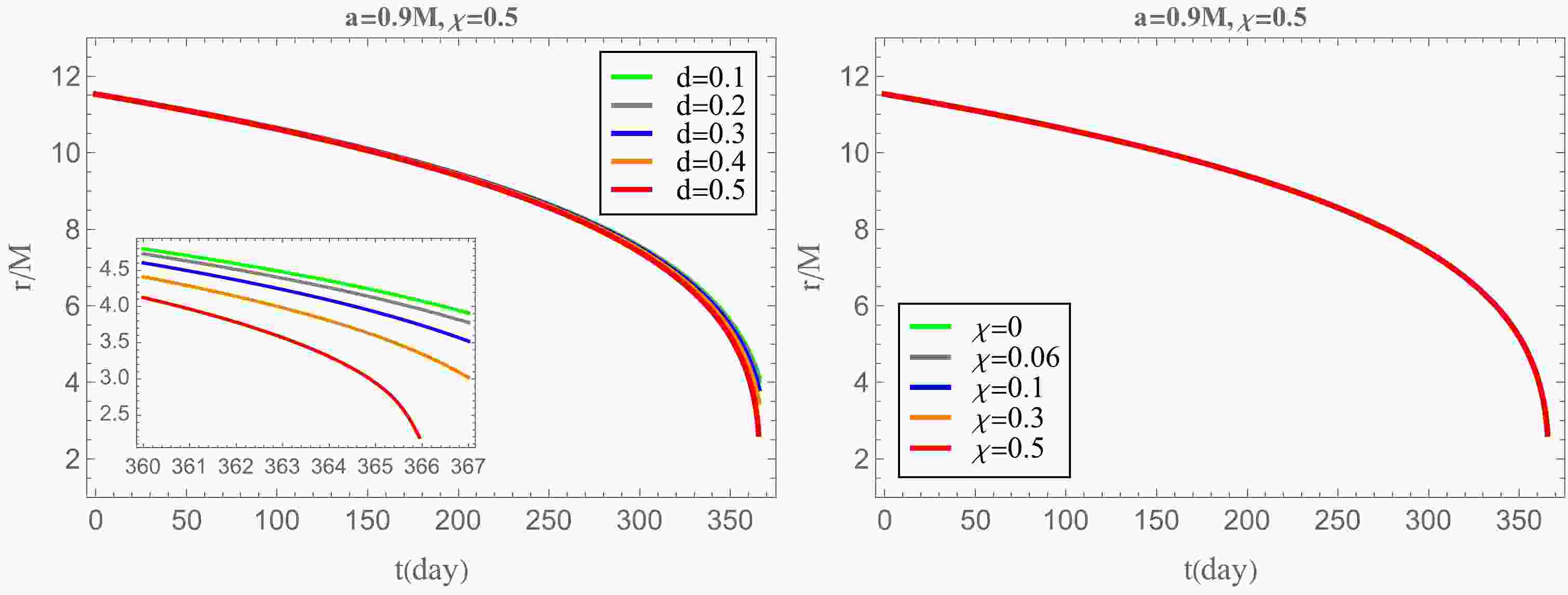
$ {\cal{O}}(1/q) $ [30], whereas the effect of the secondary spin is of higher-order with a factor of$ {\cal{O}}(q^2) $ [55]. This is demonstrated by the scalar perturbation Eq. (8), where the scalar charge appears directly in the source term, leading to a scalar radiation proportional to$ d^2 $ . In contrast, the effect of the secondary spin on scalar radiation is only reflected in the 4-velocity in Eq. (8).The adiabatic evolution of the secondary, as shown in Fig. 1, corroborates our discussion. Notably, the presence of the scalar charge d accelerates the fall of the spinning secondary into the BH, whereas the changes in the secondary spin have a negligible impact on the orbital evolution. This conclusion also applies to the behavior of the energy fluxes, as illustrated in Fig. 2 and Fig. 3. In Fig. 2, setting scalar charge
$ d=0.5 $ , an increasing secondary spin$ \chi $ has little effect on the total energy flux${\cal{F}}_{\rm tot}$ . This phenomenon becomes even more apparent when observing the ratio of total energy flux to the GR energy flux${\cal{F}}_{\rm tot}/\dot{E}_T$ in the figure at the right. However, the presence of additional scalar radiation can amplify the orbital deviations and dephasing caused by the secondary spin, as evident in Fig. 3. By fixing the secondary spin$ \chi=0.5 $ , the growth of scalar charge leads to an enlargement of the total energy flux${\cal{F}}_{\rm tot}$ , which is particularly noticeable in the ratio of total energy flux to GR${\cal{F}}_{\rm tot}/\dot{E}_T$ .
Figure 1. (color online) Fixing
$ a=0.9M $ , the radial location of the secondary$ r(t) $ as a function of the evolution time t. Left: effect of different values of scalar charge on the orbital evolution when we set$ \chi=0.5 $ . Right: effect of different values of secondary spin$ \chi $ on the orbital evolution when we set$ d=0.5 $ .
Figure 2. (color online) Fixing
$ a=0.9M $ , the total energy flux${\cal{F}}_{\rm tot}$ and relative difference between the total energy flux and gravitational energy flux${\cal{F}}_{\rm tot}/\dot{E}_T$ as a function of the orbital velocity$ v=(M\Omega)^{1/3} $ with different values of secondary spin$ \chi $ for scalar charge$ d=0.5 $ .
Figure 3. (color online) Fixing
$ a=0.9M $ , the total energy flux${\cal{F}}_{\rm tot}$ and relative difference between the total energy flux and gravitational energy flux${\cal{F}}_{\rm tot}/\dot{E}_T$ as a function of the orbital velocity$ v=(M\Omega)^{1/3} $ with different values of secondary scalar charge d for secondary spin$ \chi=0.5 $ .As we discussed earlier, the secondary spin in the EMRI system is a secondary effect that does not impact the detection of the scalar charge. Therefore, it is appropriate to overlook the influence of the secondary spin when designing the GW template for the detection of the scalar charge [56]. Interestingly, the existence of the scalar field would amplify both the deviation in the orbital evolution and the total energy radiation caused by the secondary spin, thereby improving the ability to detect the secondary spin.
This motivates us to further study GW dephasing to facilitate the detection of the secondary spin in this model. By solving the equations of adiabatic evolution (Eq. (44)), we obtain the total GW phase
$ N_{\chi}^d $ during the entire evolution. The dephasing is then calculated by$ |N_{\chi}^d-N_{\chi=0}^d| $ as a function of the secondary spin$ \chi $ for different scalar charge d. As shown in Fig. 4, the red line represents the result in GR, where the dephasing linearly increases with the secondary spin, which is consistent with the discussion in [47]. The presence of scalar charges significantly amplifies the dephasing in the model, particularly in regions where the secondary spin$ \chi $ is relatively large. This suggests that the scalar charge d can effectively improve the model's detection limit for the secondary spin$ \chi $ , as illustrated in the right figure. The phase resolution of a space-based GW detector is limited to$ \Delta\varphi\lesssim 1 $ rad by matched-filter search and parameter estimation [57]. Taking$ \Delta\varphi= 1 $ rad as a limit for the discussion, when the scalar charge is$ d=0 $ , the minimum detectable value for the secondary spin is$ \chi=0.014 $ . However, when the scalar charge is increased to$ d=0.5 $ , we can detect a spin of$ \chi=0.006 $ , which is a 133% improvement in the detection limit. The detailed data for dephasing can be found in Table 1 in Appendix A.
Figure 4. (color online) Fixing
$ a=0.9M $ , the behavior of dephasing$ |N_{\chi}^d-N_{\chi=0}^d| $ as a function of secondary$ \chi $ . The right figure is a local enlargement of the left figure in the small$ \chi $ area. The black horizontal dashed line represents the limit$ \Delta\varphi= 1 $ rad.Furthermore, the presence of the scalar field amplifies dephasing, which leads to a systematic improvement in the spin resolution of this model [47]. Considering two waveforms that differ only by the secondary spin,
$ \chi_1 $ and$ \chi_2 $ , we can evaluate the minimum detectable spin difference using the phase resolution [46, 47]:$ |\Delta \chi|=|\chi_1-\chi_2|>\frac{\Delta\varphi}{\left|\delta \varphi_{\rm{GW}}\right|}, $

(45) where
$ \Delta\varphi=1 $ rad, as constrained eailer;$ \delta\varphi_{\rm{GW}} $ can be replaced by$ N_{\chi}^d-N_{\chi=0}^d $ in this model. Figure 5 shows that the spin resolution is effectively improved by the scalar charge. As the scalar charge increases to$ d=0.5 $ , the improvement exceeds 100%. Moreover, we observe that the slope of the resolution becomes more skewed as d exceeds$ d\approx 0.45 $ . This suggests that a larger scalar charge is more beneficial for improving the spin resolution.
Figure 5. (color online) Fixing
$ a=0.9M $ , we show the spin resolution as a function of the scalar charge d for different values of secondary spin$\chi=0.1,~ 0.3,~ 0.5$ as an example.Previously, we derived exact results on how the presence of the scalar field amplifies the detection of the secondary spin in terms of detection limit and spin resolution. We now focus on assessing the detection capabilities of space-based GW detectors, particularly LISA, Taiji, and TianQin. Additional details on the calculations and related detector configurations are provided in Appendix B. In this setup, the secondary body has a mass of
$ m_p=10M_{\odot} $ with a scalar charge of$ d=0.5 $ , whereas the primary mass is$ M=4\times10^5M_{\odot} $ with spin$ a=0.9M $ .One way to quantitatively assess the detectability of a GW detector is through the faithfulness
$ {\cal{F}} $ , which compares two GW signals with and without the presence of the secondary spin. The faithfulness measures the difference between these two signals weighted by the noise spectral density of the GW detector. For example, with a signal-to-noise ratio (SNR)$ \rho=30 $ , the GW detector requires faithfulness$ {\cal{F}}\leq 0.988 $ to determine the parameter resolution of the secondary spin. Here, we calculate the faithfulness as a function of the secondary spin for two scalar charge values,$ d=0.001 $ and$ d=0.5 $ .The results illustrated in Fig. 6 demonstrate that, after one-year evolution, the faithfulness decreases with increasing secondary spin for all three GW detectors, namely, LISA, Taiji, and TianQin. In most regions of the secondary spin, the faithfulness is sufficiently small for all three GW detectors to distinguish between GW signals with and without a secondary spin. Interestingly, the value of faithfulness for
$ d=0.5 $ is consistently lower than that for$ d=0.001 $ , indicating that the GW signal for$ d= $ 0.5 is generally more favorable than that for$ d=0.001 $ . By setting the threshold at$ {\cal{F}}=0.988 $ , we can observe that the existence of the scalar charge d improves the resolution of the secondary spin. For example, for the GW detector TianQin, the resolution improves from$ \chi=0.025 $ when$ d=0.001 $ to$ \chi<0.01 $ when$ d=0.5 $ . These results support our conclusion that the presence of the scalar field enhances the detectability of the secondary spin and improves the resolution of the secondary spin for space-based detectors.
Figure 6. (color online) Faithfulness as a function of the secondary spin with
$ d=0.5 $ and$ d=0.001 $ for LISA, Taiji, and TianQin, respectively. Here, the parameters are set as$ a=0.9M $ ,$ M=4\times10^5M_\odot $ ,$ m_p=10M_\odot $ , and$r_{\rm start}=11.53M$ with one-year evolution.Moreover, when considering
$ M=4\times 10^{5}M_{\odot} $ , the faithfulness of TianQin is found to be better than that of the other two GW detectors, LISA and Taiji, as shown in Fig. 6. This is expected because the TianQin detector exhibits higher sensitivity in the high-frequency range [22]. In addition, we observe an increase in faithfulness with the growth of the primary BH mass when comparing the faithfulness of the three space-based GW detectors with primary masses of$ M=1\times10^6M_\odot $ and$ M=1\times10^7M_\odot $ in Fig. 7 and Fig. 8, respectively. Notably, for$M=1\times 10^6M_\odot$ , the presence of the scalar charge d has little effect on improving the resolution of the secondary spin$ \chi $ , whereas for$ M=1\times10^7M_\odot $ , the secondary spin$ \chi $ is indistinguishable from that in GR. This implies that the scalar radiation is more efficient in the far-field zone than in the near-field zone, as illustrated in Fig. 3, when considering gravitational radiation. When the mass of the primary BH is moderate, the evolution of the secondary begins far away from the primary BH. However, when the mass of the primary BH is considerable, the one-year evolution of the secondary occurs in the near-field zone, as noted in the captions of Fig. 7 and Fig. 8. In conclusion, the secondary spin$ \chi $ is more suitable for detection in the required region when the mass of the primary BH M is not large, and TianQin is the optimal choice for detection of the secondary spin.
Figure 7. (color online) Faithfulness as a function of the secondary spin with
$ d=0.5 $ and$ d=0.001 $ for LISA, Taiji, and TianQin, respectively. Here, the parameters are set as$ a=0.9M $ ,$ M=1\times10^6M_\odot $ ,$ m_p=10M_\odot $ , and$r_{\rm start}=7.2M$ with one-year evolution.
Figure 8. (color online) Faithfulness as a function of the secondary spin with
$ d=0.5 $ and$ d=0.001 $ for LISA, Taiji, and TianQin, respectively. Here, the parameters are set as$ a=0.9M $ ,$ M=1\times10^7M_\odot $ ,$ m_p=10M_\odot $ , and$r_{\rm start}=3.0M$ with one-year evolution. -
In this paper, we discuss the detectability of the secondary spin in the EMRI system within a modified gravity model coupled with a scalar field. The central BH, which reduces to a Kerr one, is circularly spiraled by a scalar-charged spinning secondary body on the equatorial plane. In contrast to GR, the presence of the scalar field supports an additional radiation channel for the GW, offering a modified GW template that could potentially shed light on the properties of binary systems.
This model considers a one-year adiabatic evolution starting at
$r_{\rm start}=11.53M$ for the Kerr BH with a primary spin$ a=0.9M $ and mass$ M=4\times10^5M_{\odot} $ , whereas the secondary has a mass of$ m_p=10M_{\odot} $ . By numerically solving the inhomogeneous Teukolsky equation and scalar perturbation equation, we calculate the total energy fluxes and dephasing for a range of model parameters including$ d\in[0,0.5] $ and$ \chi\in[0,0.5] $ . Our analysis of the orbital evolution and total energy fluxes confirms that the secondary spin plays a relatively secondary role in the EMRI system, suggesting a limited influence on detecting the scalar charge. Nonetheless, we determined that the inclusion of scalar radiation may enhance the detection threshold and spin resolution, as evidenced by our analysis of its overall dephasing. As shown in Fig. 4, an increase in scalar charge leads to a lower detection limit, with an improvement from$ \chi=0.014 $ for$ d=0 $ to$ \chi=0.006 $ for$ d=0.5 $ . Moreover, the spin resolution, determined by Eq. (45), is enhanced by over 100% if the scalar charge is increased to$ d=0.5 $ . A more pronounced tilt in the spin resolution slope, as depicted in Fig. 5, corroborates that a greater scalar charge confers a more substantial enhancement to the spin resolution.To validate our theoretical analysis, we calculate the faithfulness to compare the results of GW signals with and without a secondary spin. It is proved that the presence of the scalar field enhances the detectability of the secondary spin by all three space-based GW detectors. In Fig. 6, our results show that the faithfulness decreases with the growth of the scalar charge and is sufficiently small to distinguish the GW signals from GR in most regions of the secondary spin. Moreover, the value of faithfulness for
$ d=0.5 $ is always lower than that for$ d=0.001 $ , indicating an improved spin resolution that will be more precise in regions with a large secondary spin. The secondary spin detection limit of space-based detectors can be determined by the threshold at a faithfulness${\cal{F}}= 0.988$ , which is found to be improved by the scalar charge. For TianQin, as an example, the detection limit improves from$ \chi=0.025 $ when$ d=0.001 $ to$ \chi<0.01 $ when$ d=0.5 $ .Furthermore, our results show that TianQin is a better choice for detecting the secondary spin using this model, as its behavior of faithfulness is better than those of LISA and Taiji when considering the primary mass
$ M=4\times10^5M_\odot $ . This occurs because TianQin has greater sensitivity in the high-frequency region. However, as we increase the primary mass, the presence of the scalar charge has little effect on improving the resolution of the secondary spin when$ M=1\times10^6M_\odot $ , as shown in Fig. 7. Finally, the secondary spin is indistinguishable from that in GR when$ M=1\times10^7M_\odot $ , as shown in Fig. 8. This is reasonable because the scalar radiation is more effective than the gravitational radiation in the far-field zone, but the entire one-year evolution is completed in the near-field zone where the gravitational radiation grows faster [30, 32].In summary, our study investigated the detectability of the secondary spin in the modified gravity model coupled with a scalar field. We found that the presence of the scalar field amplifies the secondary spin effect, allowing for the detection of a lower limit value of the secondary spin and an improved resolution of secondary spin detection when the scalar charge is sufficiently large. Our findings suggest that the secondary spin is more suitable for detection when the primary mass is not large, and TianQin is the optimal choice for detection.
The implications of our results are crucial for future observations of EMRIs and for testing modified gravity theories in the strong field regime. They suggest that the presence of scalar fields could substantially impact the dynamics of compact objects in the vicinity of supermassive BHs, leading to important consequences for interpreting GW signals. Moreover, our study supports that the EMRI model in modified gravity theories can enable investigations onto the properties of binaries. This is an important direction for future research, as alternative theories of gravity may offer a better tool for exploring the universe than GR. Consequently, we can further discuss the constraints on cosmological parameters [58, 59] and detection of model parameters [60, 61]. In addition, the interaction between the secondary spin and the scalar field should be considered for further precise discussion on the detection of the secondary spin (we considered only the simplest case in this study). Finally, other modified gravities may have additional radiations, making the study of EMRI systems in these models valuable for future research.
This study represents an initial step toward detecting the spin of secondary objects with the extra contribution from scalar radiation of GWs in EMRIs. Future extensions to the generic orbital motion represent a crucial direction for achieving consistency with the exact astrophysical environment and the facts of complex dynamics of the secondary objects. One way to consider the dynamic characteristics of spin particles deviating from the equatorial plane is by keeping the linear-in-spin approximation of the MPD equations, considering
$ \sigma\ll 1 $ for the secondary spin [62, 63]. Under this assumption, integrability is approximately maintained at$ {\cal{O}}(\sigma) $ owing to the approximately conserved quantities [64], at least for the Tulczyjew-Dixon equation (Eq. (11)). A Carter-like constant remains conserved at order$ {\cal{O}}(\sigma) $ [65, 66]. However, a challenge arises due to the absence of a strict flux-balance law for this approximately conserved quantity [44]. Further, a precise assessment of the detectability of the secondary spin by upcoming interferometers would necessitate a statistical analysis grounded in Bayesian inference. Owing to the intricacy and slow generation of EMRI waveforms computed by BH perturbation theory, the discussion of faithfulness is a preliminary analysis of the parameter estimation for this model. EMRI detection and parameter estimation with the future interferometers require accurate waveform models that include the relevant self-force terms. It is thus reasonable to discuss the parameter estimation through a Monte Carlo simulation or Fisher matrix. The parameter degeneracy can be further explored in the future, especially with an account of the leading-order conservative corrections from the self-force [55, 67, 68] as well as the dissipative effects [44, 69, 70] sourced by second order metric perturbations. -
We can obtain the inspiral trajectory from adiabatic evolution in Eq. (44). Then, it is convenient to compute GW waveforms in the quadrupole approximation. The metric perturbation in transverse-traceless (TT) gauge is
$ h_{i j}^{\rm{TT}}=\frac{2}{d_L}\left(P_{i l} P_{j m}-\frac{1}{2} P_{i j} P_{l m}\right) \ddot{I}_{l m} , $

(A1) where
$ d_L $ is the source luminosity distance,$ P_{ij}=\delta_{ij}-n_i n_j $ is the projection operator on the wave unit direction$ n_j $ , and$ \delta_{ij} $ is the Kronecker delta function.$ \ddot{I}_{ij} $ is the second time derivative of the mass quadrupole moment, which is given in terms of the source stress-energy tensor$ I_{i j}=\int d^{3} x T_p^{t t}\left(t, x^{i}\right) x^{i} x^{j}=m_p y_p^{i}(t) y_p^{j}(t), $

(A2) where the stress-energy tensor component
$ T_p^{tt} $ is as expressed in Eq. (5). Thus, the strain produced by the GW, as measured by the detector, is given by$ h(t)=h_+(t) F^+(t)+h_\times(t) F^\times(t), $

(A3) where
$ h_+(t)={\cal{A}}\cos\left[2\varphi_{\rm orb}+2\varphi_0\right]\left(1+\cos^2\iota\right) $ ,$ h_\times(t)= -2{\cal{A}}\sin\left[2\varphi_{\rm orb}+2\varphi_0\right]\cos\iota $ , and$ \iota $ is the inclination angle between the binary orbital angular momentum and the line of sight. The GW amplitude$ {\cal{A}}=2m_{\rm p}\left[M\Omega(t)\right]^{2/3}/d_L $ , where$ d_L $ is the luminosity distance. The interferometer pattern functions$ F^{+,\times}(t) $ and$ \iota $ can be expressed in terms of four angles, which specify the source orientation$ (\theta_s,\phi_s) $ and orbital angular direction$ (\theta_1,\phi_1) $ . -
In the time domain, we can use twelve parameters
$\vec{\xi}=({\rm ln}\; M, {\rm ln}\; m_p, a, \chi, d, r_0, \varphi_0, \theta_s, \phi_s, \theta_1, \phi_1, d_L)$ to determine the GW waveform (B3). Here, we fix the source angles$ \theta_s=\pi/3,\; \phi_s=\pi/2 $ , and$ \theta_1=\phi_1=\pi/4 $ . The initial phase is set as$ \varphi_0=0 $ , the initial orbital separation is set to$r_{\rm start}=11.53M$ , and one-year adiabatic evolution is considered before the plunge$r_{\rm ISCO}$ . As mentioned above, we consider the model with$ m_p=10M_{\odot} $ ,$ M=4\times10^5M_{\odot} $ , and$ a=0.9M $ . Here, we choose$ d=0.5 $ to vary the secondary spin$ \chi $ , and the luminosity distance$ d_L $ is a free scale factor for$ h(t) $ .The noise-weighted inner product between two templates is introduced:
$ \langle h_{1} \mid h_{2}\rangle=4 \Re \int_{f_{\min }}^{f_{\max }} \frac{\tilde{h}_{1}(f) \tilde{h}_{2}^{*}(f)}{S_{n}(f)} {\rm d} f, $

(A4) $ \tilde{h}_{1}(f) $ is the Fourier transform of the time domain signal, and its complex conjugate is$ \tilde{h}_{2}^{*}(f) $ .$ S_n(f) $ is the noise spectral density, the value of which is provided in the next subsection for LISA, Taiji, and TianQin.Notice that the signal (B3) is sampled in the time domain, which will be applied by a discrete Fourier transform evaluating the integral (B4) between
$f_{\min}=10^{-4}$ Hz and$f_{\max}=f_{N}$ . Here,$ f_N $ is the Nyquist frequency. The component related to the latter is set to zero, and only$f\geq f_{\min}$ Fourier components are included. Before passing to the frequency space, we taper$ h(t) $ with a Tukey window with cosine fraction$ \tau = 0.05 $ . The signal-to-noise ratio (SNR) can be obtained by$ \rho=\langle h|h \rangle^{1/2} $ . The faithfulness between two GW signals is determined by$ {\cal{F}}\left[h_1, h_2\right]=\max _{\left\{t_c, \phi_c\right\}} \frac{\langle h_1 \mid h_2\rangle}{\sqrt{\langle h_1 \mid h_1\rangle\langle h_2 \mid h_2\rangle}}, $

(A5) where
$ (t_c, \varphi_c) $ are time and phase offsets. -
As discussed above, the GW strain signal detected in a space-based GW detector is expressed in Eq. (B3), where the antenna pattern functions
$ F^{+,\times} $ describing the detector response to sources with different locations and polarizations are given by$ \begin{aligned}[b]F^+_1\left(\theta_{s}, \phi_{s}, \psi_{s}\right)=\;&\frac{\sqrt{3}}{2}\left[\frac{1}{2}\left(1+\cos ^{2} \theta_{s}\right) \cos 2 \phi_{s} \cos 2 \psi_{s}\right.\\&\left.-\cos \theta_{S} \sin 2 \phi_{s} \sin 2 \psi_{s}\right], \\ F^\times_1\left(\theta_{s}, \phi_{s}, \psi_{s}\right)=\;&\frac{\sqrt{3}}{2}\left[\frac{1}{2}\left(1+\cos ^{2} \theta_{s}\right) \cos 2 \phi_{s} \sin 2 \psi_{s}\right.\\&\left.+\cos \theta_{s} \sin 2 \phi_{s} \cos 2 \psi_{s}\right], \end{aligned} $

(A6) and the antenna pattern function of the second orthogonal Michelson interferometer can be written as
$ \begin{aligned}[b]F_{2}^+\left(\theta_{s}, \phi_{s}, \psi_{s}\right)=\;&F_{1}^+\left(\theta_{s}, \phi_{s}-\frac{\pi}{4}, \psi_{s}\right), \\ F_{2}^\times\left(\theta_{s}, \phi_{s}, \psi_{s}\right)=\;&F_{1}^\times\left(\theta_{s}, \phi_{s}-\frac{\pi}{4}, \psi_{s}\right). \end{aligned} $

(A7) Here,
$ (\theta_s,\phi_s) $ describes the source location of EMRIs in the sky, and the polarization angle function can be expressed as$ \tan \psi_{S}=\frac{\hat{L} \cdot \hat{z}-(\hat{L} \cdot \hat{N})(\hat{z} \cdot \hat{N})}{\hat{N} \cdot(\hat{L} \times \hat{z})}, $

(A8) where
$ \hat{L} $ and$ -\hat{N} $ are the unit vector along the orbital angular momentum and direction of GW propagation, respectively. Then, the Doppler phase due to the detector's orbital motion into the GW signal is$ \varphi_{\text {orb}}(t) \rightarrow \varphi_{\text {orb }}(t)+\frac{d \varphi_{\text {orb }}(t)}{d t} R_{\rm{AU}} \sin \theta_{s} \cos \left(2 \pi t /(1 \text { year })-\phi_{s}\right). $

(A9) Now, we introduce the power spectral density (PSD) values of LISA and Taiji, which consist of the instrumental and confusion noise produced by unresolved galactic binaries [71, 72]:
$\begin{aligned}[b] S_{n}^{\rm LISA,Taiji}(f)=\;& \frac{10}{3 (L^{L,T})^{2}}\left[P_{\rm{OMS}}^{\rm LISA,Taiji}+2\left(1+\cos ^{2}\left(f / f_{*}\right)\right) \right.\\&\times\left.\frac{P_{\rm{acc}}}{(2 \pi f)^{4}}\right] \left[1+\frac{6}{10}\left(\frac{f}{f_{*}}\right)^{2}\right],\end{aligned} $

(A10) where
$f_*=c/(2\pi L^{\rm LISA,Taiji} )$ is the transfer frequency, and the arm length of the space-borne GW detector is given by$ L^{L}=2.5\times10^6 $ km for LISA and$ L^{T}=3\times10^6 $ km for Taiji. We have$\begin{aligned}[b] P_{\rm{acc}}=\;&(3 \times 10^{-15} {\rm{m}} / {\rm{s}}^{2})^2 \left[1+\left(\frac{0.4 {\rm{mHz}}}{f}\right)^{2}\right]\\&\times \left[1+\left(\frac{f}{8 {\rm{mHz}}}\right)^{4}\right]{\rm{Hz}}^{-1}\end{aligned} $

(A11) $ \begin{aligned}[b]& P_{\rm{OMS}}^{\rm{LISA}}=(1.5 \times 10^{-11} {\rm{m}})^2 \left[1+\left(\frac{2 {\rm{mHz}}}{f}\right)^{4}\right]{\rm{Hz}}^{-1}, \\& P_{\rm{op}}^{\rm{Taiji}}=(8 \times 10^{-12} {\rm{m}})^2 \left[1+\left(\frac{2 {\rm{mHz}}}{f}\right)^{4}\right] {\rm{Hz}}^{-1}. \end{aligned} $

(A12) The sky averaged sensitivity of TianQin is in [73]
$ \begin{aligned}[b]& S_{n}^{\rm TianQin}(f)=\frac{S_{N}^{\rm TianQiin}(f)}{\bar{R}(2 \pi f)} \\& S_{N}(f)=\frac{1}{(L^{TQ})^{2}}\left[\frac{4 S_{a}}{(2 \pi f)^{4}}\left(1+\frac{10^{-4}\;{\rm Hz}}{f}\right)+S_{x}\right] \\& \bar{R}(w)=\frac{3}{10} \times \frac{g(w \tau)}{1+0.6(w \tau)^{2}} , \end{aligned} $

(A13) where
$ L^{TQ}=\sqrt{3}\times10^5 $ km,$ S_{a}^{1 / 2}=1 \times 10^{-15} \; {\rm{m}} \; {\rm{s}}^{-2} \; {\rm{Hz}}^{-1 / 2}, S_{x}^{1 / 2}=1 \times 10^{-12} \; {\rm{m}} \; {\rm{Hz}}^{-1 / 2} $ .$ \tau=L^{TQ}/c $ is the travel time for the TianQin arm length and$\begin{aligned}[b]& g(x)=\\&\left\{\begin{array}{cc} {\sum\nolimits_{i=0}^{11} a_{i} x^{i} }& {: \quad x<4.1} \\ {\exp [-0.322 \sin (2 x-4.712)+0.078]} & {: 4.1 \leq x<\dfrac{20 \pi}{\sqrt{3}}} \end{array}\right. \end{aligned}$

(A14) with
$ (a_0,a_1,a_2,a_3,a_4,a_5,a_6,a_7,a_8,a_9,a_{10},a_{11})$ =$(1,10^{-4}, 0.2639,\;4.62\times10^{-3},\;-0.16744,\;2.173\times10^{-2},\;2.101\times10^{-3}$ ,$1.5135\times 10^{-2},-8.4746\times10^{-3},1.76087\times10^{-3},-1.6046\times10^{-4}, 5.169\times10^{-6}) $ .
Detecting secondary spin with extreme mass ratio inspirals in scalar-tensor theory
- Received Date: 2024-04-13
- Available Online: 2024-09-15
Abstract: In this study, we investigate the detectability of the secondary spin in an extreme mass ratio inspiral (EMRI) system within a modified gravity model coupled with a scalar field. The central black hole, which reduces to a Kerr one, is circularly spiralled by a scalar-charged spinning secondary body on the equatorial plane. The analysis reveals that the presence of the scalar field amplifies the secondary spin effect, allowing for a lower limit of the detectability and an improved resolution of the secondary spin when the scalar charge is sufficiently large. Our findings suggest that secondary spin detection is more feasible when the primary mass is not large, and TianQin is the optimal choice for detection.


 DownLoad: