Quasinormal modes and isospectrality of Bardeen (Anti-) de Sitter black holes

Over the years, the gravitational wave searches for the coalescence of compact binaries [1] and the shadow images captured by the Event Horizon Telescope [2, 3] explicitly provide evidence of the existence of BHs. In general relativity, essential singularities, which cannot be eliminated by coordinate transformation, are present in BHs. Modern physics tries to construct a complete theory of quantum gravity and understand the microscopic mechanism of BHs. However, the description of the essential singularity has encountered enormous difficulties. To overcome this problem, one can consider that the BHs without essential singularities are known as regular black holes. Compared with those of singular black holes, regular black holes exhibit some new phenomena, which have recently attracted significant attention [4]. This kind of solution was first proposed by Bardeen [5]. Ayón-Beato and García found that, to obtain a regular black hole solution, the energy-momentum tensor should be the gravitational field of some magnetic monopole generated by a specific form of nonlinear electrodynamics [6−8]. Since then, numerous researchers have contributed various singularity-free solutions [9−14], which have attracted increasing attention in recent years [15−17].

In the context of binary black hole coalescence, the process can be divided into three distinct stages: inspiral, merge, and ringdown, each calculated using different methods. The inspiral can be discussed by the post-Newtonian approximation, and the merge is always calculated using numerical calculation. The final stage is equivalent to making a perturbation to the equilibrium state of the black hole. This stage corresponds to damped oscillations with complex frequencies, which always depend only on the black hole properties, such as mass, charge, and angular momentum. These modes are called quasinormal modes (QNMs). The gravitational perturbation equations for the axial sector of Schwarzschild spacetime were initially formulated by Regge and Wheeler [18] and later extended to the polar sector by Zerilli [19, 20]. Extensive research has been dedicated to numerically determining the quasinormal frequencies (ω) for various scenarios. It is well-established that the axial and polar gravitational perturbations of asymptotically flat spacetime, such as those associated with Schwarzschild or Reissner-Nordström BHs, exhibit isospectrality [21]. Conversely, the investigation of quasinormal modes in asymptotically Anti-de Sitter (AdS) spacetime has attracted significant interest owing to the AdS/CFT duality [22, 23]. Numerical investigations have revealed a distinct parity splitting phenomenon for Schwarzschild-AdS BHs [24]. Furthermore, in addition to their classical properties, quasinormal modes also exhibit intriguing quantum characteristics inherent to BHs [25, 26].

After the Bardeen solution was presented, many studies focused on the perturbation problem of the Bardeen BHs. The QNMs due to the neutral or charged scalar field perturbation for regular black holes have been discussed in Refs. [27, 28]. Ulhoa investigated the axial gravitational perturbations of a regular black hole [29]. To investigate the stability of nonlinear electrodynamic black holes, Moreno and Sarbach derived the perturbation equations [30]. Based on this result, Chaverra et al. calculated the QNMs of black holes in nonlinear electrodynamics and discovered that parity splitting exists for the alternative model to the Bardeen black hole [31]. Further, Toshmato et al. studied the electromagnetic perturbation of black holes coupled with nonlinear electrodynamics, and their results show a correspondence between the axial and polar parts of electromagnetic perturbations of electrically charged or magnetically charged black holes [32, 33]. The Dirac QNMs of regular black holes were also investigated in [34].

The Bardeen BH with cosmological constant was initially introduced by Fernando [35]. In this study, we derive the master variables and corresponding master equations for the gravitational perturbations of Bardeen (Anti-) de Sitter BHs, employing the so-called A-K notation. Our analysis encompasses both the axial (odd-parity) and polar (even-parity) sectors. Subsequently, we numerically compute the QNMs with the necessary analysis. The structure of the paper is outlined as follows: In the subsequent section, we provide a brief overview of the Bardeen BH solutions and the construction of master equations for (axial and polar) gravitational perturbations. Section III focuses on the study of QNMs for the Bardeen de Sitter BH utilizing the 6th-order WKB approach. Additionally, we present a comparative discussion regarding the quasinormal frequency splitting phenomenon. Moving on to Section IV, we employ the HH method to calculate the QNMs of the Bardeen Anti-de Sitter BH. Finally, Section V is dedicated to summarizes our findings and provides a comprehensive discussion. Throughout our study, we chose $ c=G=1 $ and ignored the factor $ \kappa=8\pi $ in gravitational equations.

First, we briefly introduce the Bardeen de Sitter BH following the work in Ref. [35]. The action is given by

where $ \mathcal{L}(F)=\dfrac{3}{2 \alpha q^2}\left(\frac{\sqrt{2q^{2}F}}{1+\sqrt{2q^2F}}\right)^{5/2} $ is the Lagrangian of the nonlinear electromagnetic field strength F, and R and Λ are the scalar curvature and cosmological constant, respectively. The parameter α in $ \mathcal{L}(F) $ is related to the magnetic charge q and the mass M of the space time as follows: $ \alpha=q/2M $. The field strength F can be written as

where $ F_{\mu\nu}=\nabla_{\mu}A_{\nu}-\nabla_{\nu}A_{\mu} $. The only non-vanishing component of $ F_{\mu\nu} $ for spherically symmetric spacetime is $ F_{23}=q\sin\theta $, and then $ F=q^2/2r^4 $.

Taking the variation of the action, the equation of motion can be expressed as

The static spherically symmetric solution is given by [35]

where $ f(r)=1-\dfrac{2Mr^2}{(r^2+q^2)^{\frac{3}{2}}}-\dfrac{\Lambda r^{2}}{3} $. Here, M and q are the total mass and the magnetic charge of the Bardeen de Sitter BH. The $ \Lambda>0 $ case represents the Bardeen de Sitter BH, and the $ \Lambda<0 $ case represents the Bardeen Anti-de Sitter BH.

The decomposition of perturbed metric was first presented by Regge and Wheeler. The perturbed metric can be written as

where $ \bar g_{ab} $ denotes the metric of the background spacetime. For spherically symmetric spacetime, $ h_{ab} $ can be decomposed to the axial part and polar part under the Regge-Wheeler gauge. In this study, we use the A-K notation to decompose $ h_{ab} $ [36], which helps to give the perturbed source terms. Note that when calculating the QNMs, we do not need the source term. However, here, we present the master equation with the source term to provide some basis for studying the self-force or extreme mass ratio inspiral problems for Bardeen (Anti-)de Sitter black holes. As such, the complete basis on the two-sphere is constructed by a 1-scalar spherical harmonic, $ Y_{lm}=Y_{lm}(\theta,\varphi) $, three pure-spin vector harmonics, and six tensor harmonics [37]. The vector harmonics are defined as

and the tensor harmonics are defined as

where $ v_a=(-1,0,0,0) $ and $ n_a=(0,1,0,0) $ are two orthogonal co-vectors, $ \Omega_{ab} $ is the projection operator defined as $ \Omega_{ab}=r^2 \text{diag}(0,0,1,\sin^2\theta) $, $ \epsilon_{abc} $ represents the spatial Levi-Civita tensor $ \epsilon_{abc}\equiv v^d\epsilon_{dabc} $, and $ \epsilon_{tr\theta\varphi}=r^2\sin\theta $. Now, $ h_{ab} $ can be decomposed as

where the coefficients of each term in the above equation are all scalar functions of t and r. Hence, the polar and axial parts of $ h_{ab} $ can be written as

where

Assuming that the value of charge q is fixed, taking the variation of Eq. (3), we obtain

where

Projecting the above equations to the A-K directions, one can get the projection equations $ E_\mathrm{A}-E_\mathrm{K} $. The explicit expression of $ E_\mathrm{A}-E_\mathrm{K} $ will be placed in Appendix A.

For spherically symmetric spacetimes, there are several gauge choices [18]. In this study, we choose the RW gauge, i.e., the gauge vector $ \xi_a $ , as

which yields $ \mathrm{B}=\mathrm{F}=\mathrm{H}=\mathrm{G}=0 $. Then, the polar and axial sectors of $ h_{ab} $ become

Then, we construct the master variables and master equations for the axial or polar part, respectively. For the axial part, let

and $ \psi^{(-)} $ be satisfied

with

and

where $ \lambda=l(l+1) $.

For the polar part, we choose the gauge invariants χ and φ, defined as [38]

Note that here, $ \Lambda(r) $ is the metric function mentioned in [38], rather than the cosmological constant. Then, the master variable $ \psi^{(+)} $ can be constructed as

which satisfies the polar sector equation as

with

where the parameters N, σ, τ, $ c_1 $, and $ c_0 $ as well as $M_{\rm F}$, $N_{\rm A}$, and $N_{\rm F}$ are all the functions of background. The explicit expression of these functions can be found in Appendix B. It is easy to check that the above results can be reduce to those of GR when $ q=0 $.

Calculating the QNM, we set the source term to vanish and consider the variable $ \psi^{(\pm)}=\psi^{(\pm)}(r) {|rm e}^{-{\rm i}\omega t} $. The axial sector Eq. (18) can be directly written as the Schrödinger-like equation with an effective potential,

with

where ω is the quasinormal frequency, which indicates that the black hole will oscillate under gravitational perturbations. However, for the polar sector, Eq. (23) can be denoted as

where

and following the standard steps presented in [39], the standard Schrödinger-like equation is given by

where

and

meanwhile the potential in Eq. (29) reads as

In this section, we calculate the QNMs of the gravitational perturbation of the Bardeen de Sitter spacetime as a function of the magnetic charge q and the cosmological constant by applying the sixth-order WKB approach. The WKB approximation is one of the most widely used methods for calculating the QNMs of BHs. This method, which employs a semianalytic technique, is designed to solve the problem of scattered waves near the peak of the potential barrier $ V(r_0) $ in quantum mechanics [40−45]. Since the complete expression of the potential $ V^{(+)} $ in Eq. (29) is too complex, we expand the wave equations up to the fourth order of q in the following calculations. Hence, $ f(r) $ and $ \mathcal{L} $ can be rewritten as

In the following subsection, the numerical results show that the 4th order expansion of q has enough accuracy for our discussion. However, in order to improve the computational accuracy, we expand $ f(r) $ and $ \mathcal{L} $ to the 10th order of q in our calculation program.

Here, we use the sixth-order WKB approach to calculate the QNMs for the Bardeen de Sitter BH. For general potential $ V(r) $, the sixth order formula is given by

where

$r_{\max}$, corresponding to the maximum value of the potential V, n, is the overtone number, which can be set as $ n=0,1,2... $. The explicit expressions of $ \Lambda_{2} $ and $ \Lambda_{3} $ can be found in [41, 42], and $ \Lambda_{4} $, $ \Lambda_{5} $, and $ \Lambda_{6} $ can be found in [43].

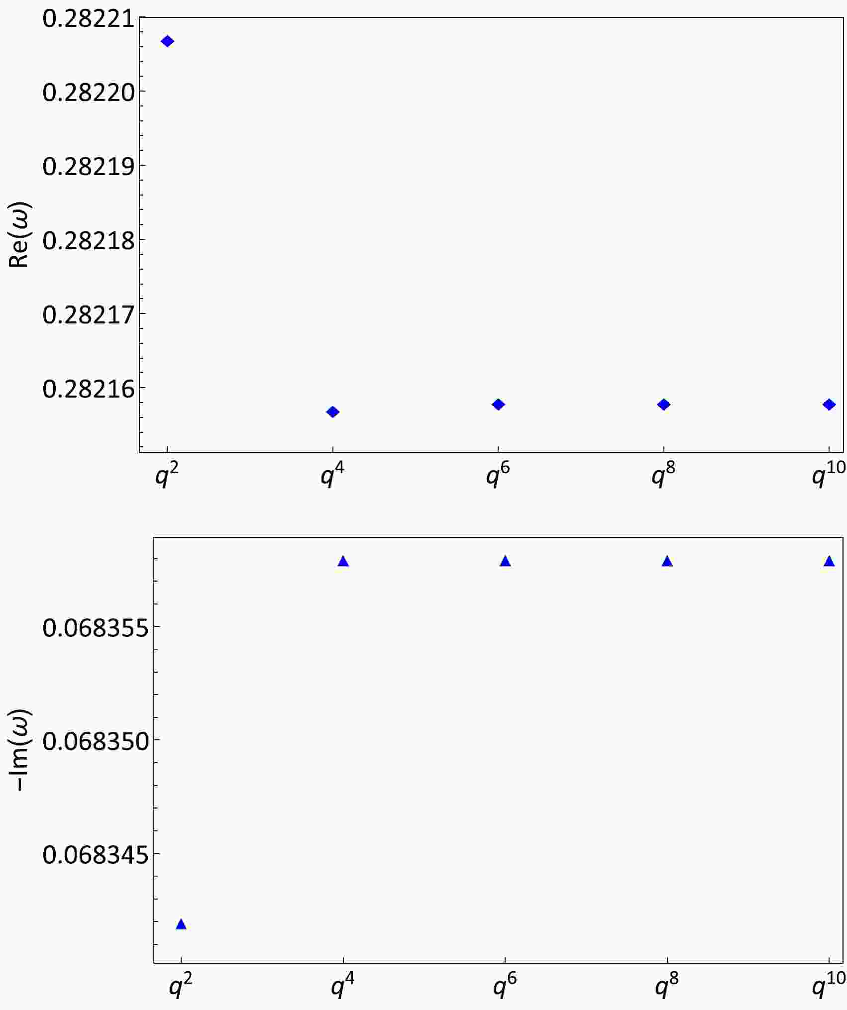
The gravitational modes exist for $ l\geq2 $. In de Sitter spacetime, we set $ M=1 $. Figure 1 describes the QNMs of axial gravitational perturbation when expanding to various orders of q. For polar gravitational perturbation, the results also indicate similar convergent behavior. It shows that expanding to the fourth order of q is sufficient, i.e., Eqs. (33) and (34) are valid in our calculation.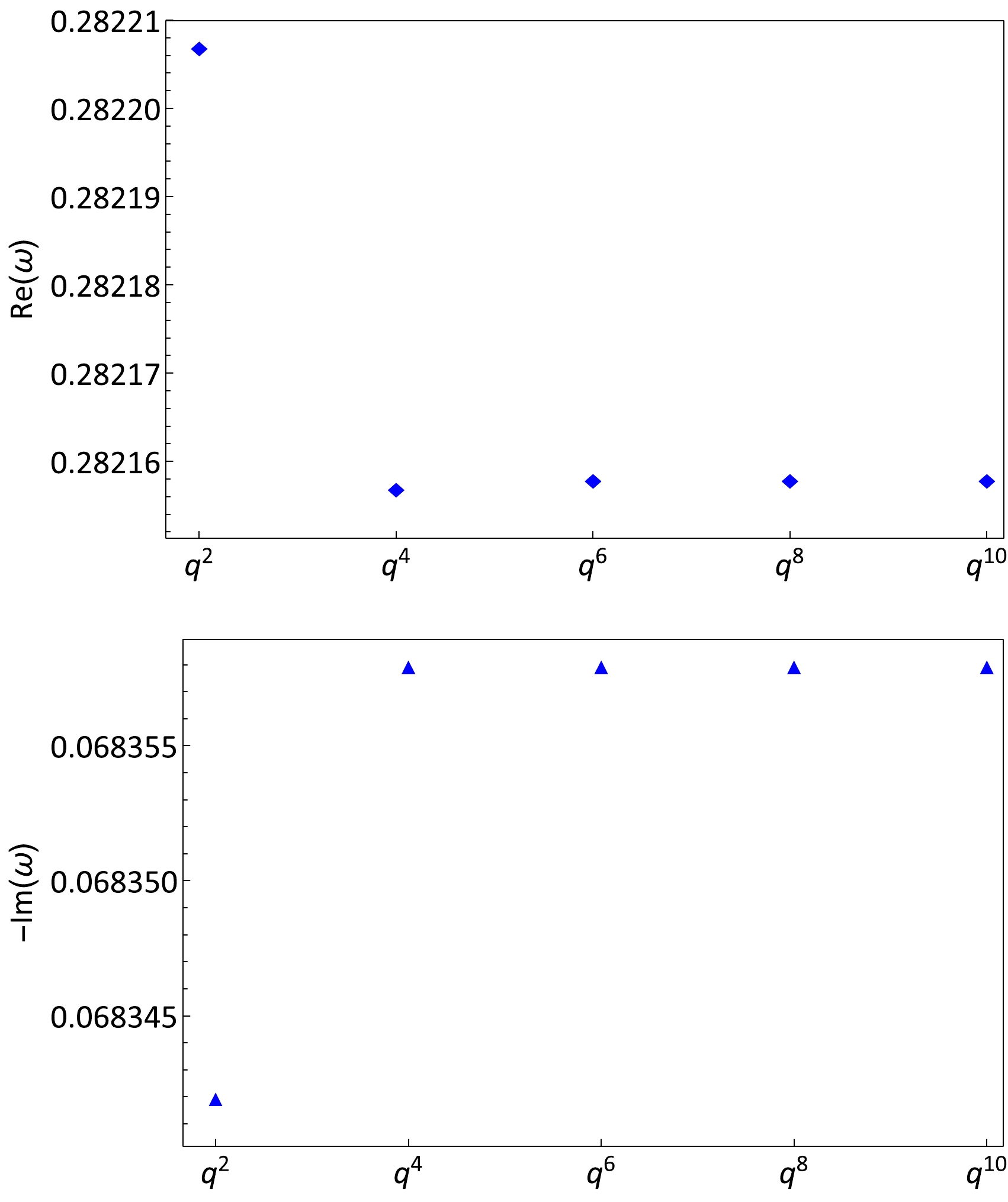

Figure 1.  (color online) QNMs of axial gravitational perturbation for varying the expanding order of q. Here, we set $ l=2 $, $ n=0 $, $ q=0.2 $, and $ \Lambda=0.05 $.

Figure 2 and Fig. 3 show the QNMs of the axial and the polar parts of the gravitational perturbation for $ l=2 $ and $ n=0 $, respectively. The figures reveal that, when q increases, the real part increases, but the magnitude of the imaginary part decreases first and then increases. The specific data for the QNM frequencies are presented in Appendix C. The data in Table 2 indicate that the breaking of isospectrality of QNMs exists in the Bardeen de Sitter BH.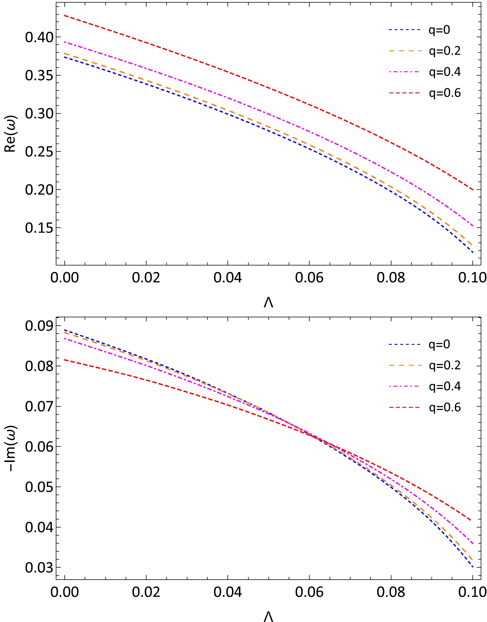

Figure 2.  (color online) QNM frequencies of the axial gravitational perturbation of the Bardeen de Sitter BHs for $ l=2,n=0 $.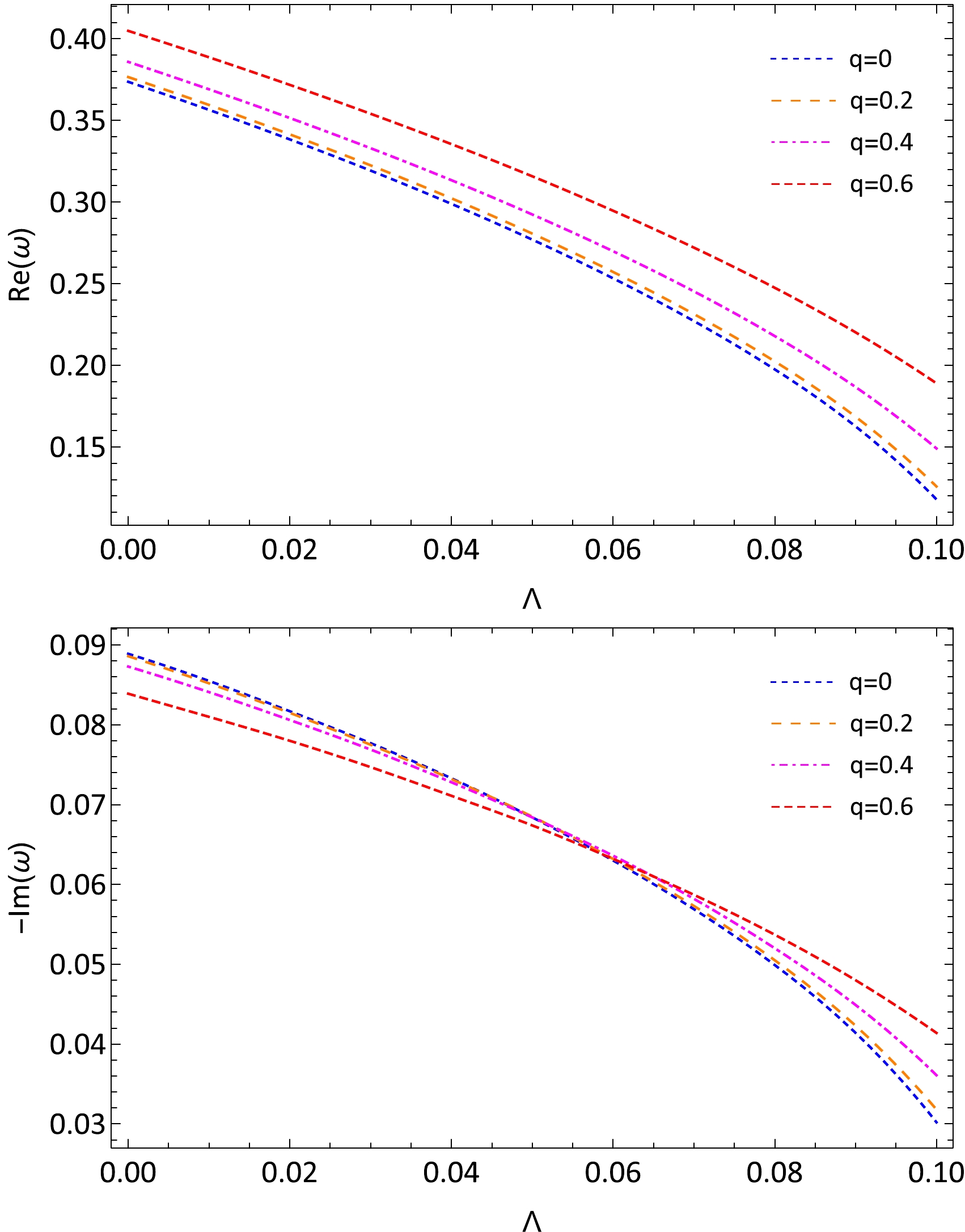

Figure 3.  (color online) QNM frequencies of the polar gravitational perturbation of the Bardeen de Sitter BHs for $ l=2,n=0 $.

One should confirm that the WKB approach does not cause this breaking of isospectrality. We calculate the QNMs using various orders of the WKB approach and find that the error due to considering various orders of the WKB approach is much smaller than the breaking of isospectrality when $ q=0.6 $. Therefore, we consider that the axial and the polar gravitational perturbations of Bardeen de Sitter BHs are not isospectral.

In Fig. 4, we show the relative gap between the axial gravitational and the polar gravitational QNM frequencies, where $ \Delta\omega $ is defined as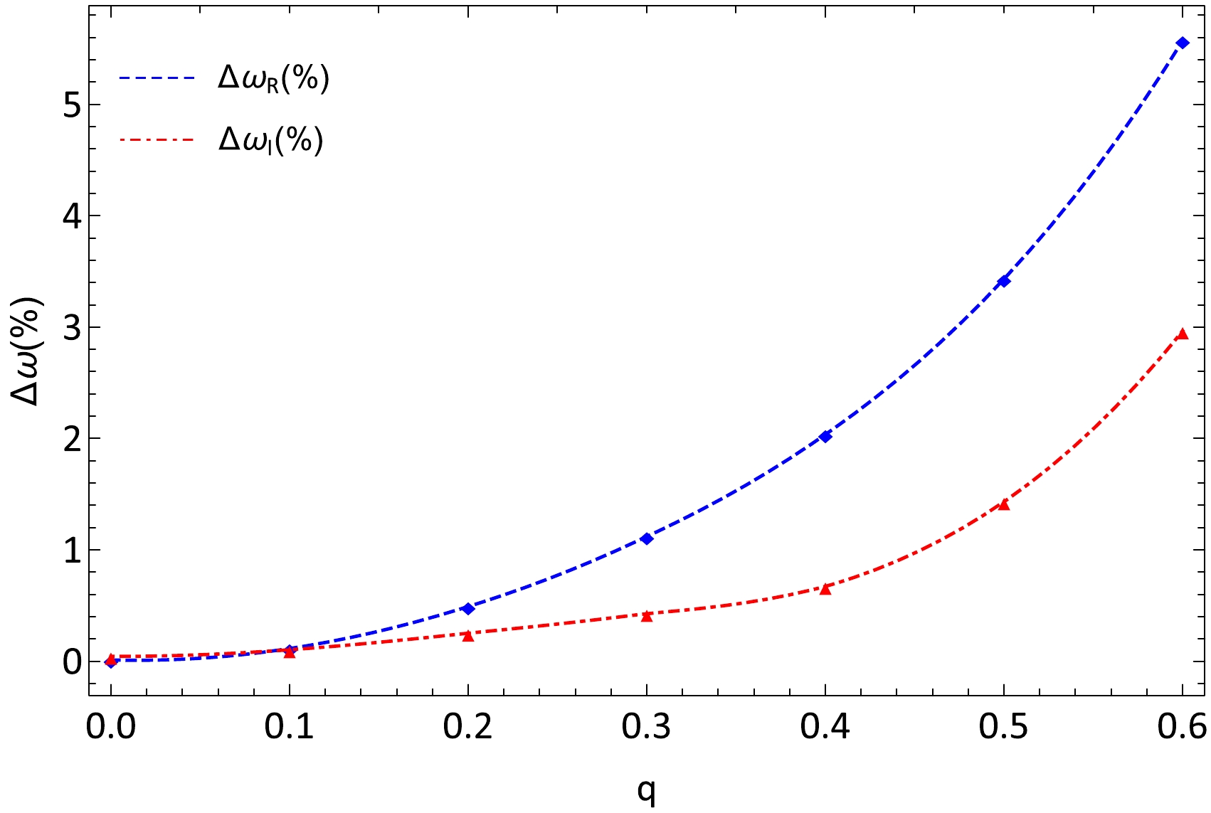

Figure 4.  (color online) The relative gap between the axial and polar QNMs of Bardeen de Sitter BHs with $ \Lambda=0.02 $ and $ l=2, n=0 $.

This result clearly shows that isospectrality will break in Bardeen de Sitter spacetime as charge q increases. However, when l is sufficiently large, our numerical results show that the frequency spectra for the axial and polar gravitational perturbations converge. This implies that isospectrality will tend to be preserved for large l's.

For the Bardeen Anti-de Sitter BH, we use the HH method to calculate the QNMs [23, 24]. A brief introduction to this method is as follows: In the HH method, the condition $ M=1 $ no longer holds. For the axial sector, we write $ \phi^{(-)} $ for a generic wavefunction as

the Schrödinger-like equation becomes

For the polar sector, from Eq. (29), we consider that $ \phi^{(+)} $ can be written as

and satisfied by

where

Then, introducing a transformation $ x=1/r $ to restrict the studied region $ r_{h}<r<\infty $ to a finite region $ 0<x<x_{h} $ and expanding Eqs. (39) and (41) at the horizon $ x_h $, we obtain

The coefficient functions $ s(x) $, $ t(x) $, and $ u(x) $ can be expanded at horizon $ x=x_h $,

and similarly for $ t(x) $ and $ u(x) $. Note that $ u(x_h)=0 $ yields $ u_0=0 $. After that, we consider the solution for Eqs. (39) and (41),

and Eq. (43) gives

where

Using the boundary condition $ \phi=0 $ at infinity, i.e., $ x=0 $,

The problem is now reduced to that of finding a numerical solution of Eq. (48). Since one cannot get a full sum from $ 0 $ to infinity, the summation should be cut off at an appropriate position N. Taking a partial sum from $ 0 $ to N, the numerical roots for $ \omega_N $ of Eq. (48) can be evaluated by some numerical method. Then, we move on to the case that takes a partial sum from $ 0 $ to $ N+1 $, and similarly determine $ \omega_{N+1} $. Comparing $ \omega_N $ and $ \omega_{N+1} $ can help us determine N to achieve a certain computational accuracy. It shows that when $ N=50 $ for axial perturbation or $ N=150 $ for polar perturbation, the calculation accuracy has three significant digits. Note that in Bardeen Anti-de Sitter spacetime, we set $ \Lambda=-3 $.

Here, we use the HH method to calculate the QNMs of the Bardeen Anti-de Sitter BH and study the influence of magnetic charge q on QNMs. The range of $ r_h $ is limited to $ r_{h}\in\left[1,100\right] $. The specific data are placed in Appendix C. Figure 5 and Fig. 6 show the axial and polar parts of the gravitational QNM frequencies for Bardeen Anti-de Sitter spacetime. For the axial gravitational perturbation, we only consider the range $ \log{r_h}\in [0.4, 0.7] $ to obviously show that as the charge q increases, the real part of ω will decrease, and the magnitude of imaginary part of ω will increase. However, for the polar gravitational perturbation, we only consider the range $ \log{r_h}\in [1.5, 2.0] $, where the deviations due to the presence of charge q can be clearly seen.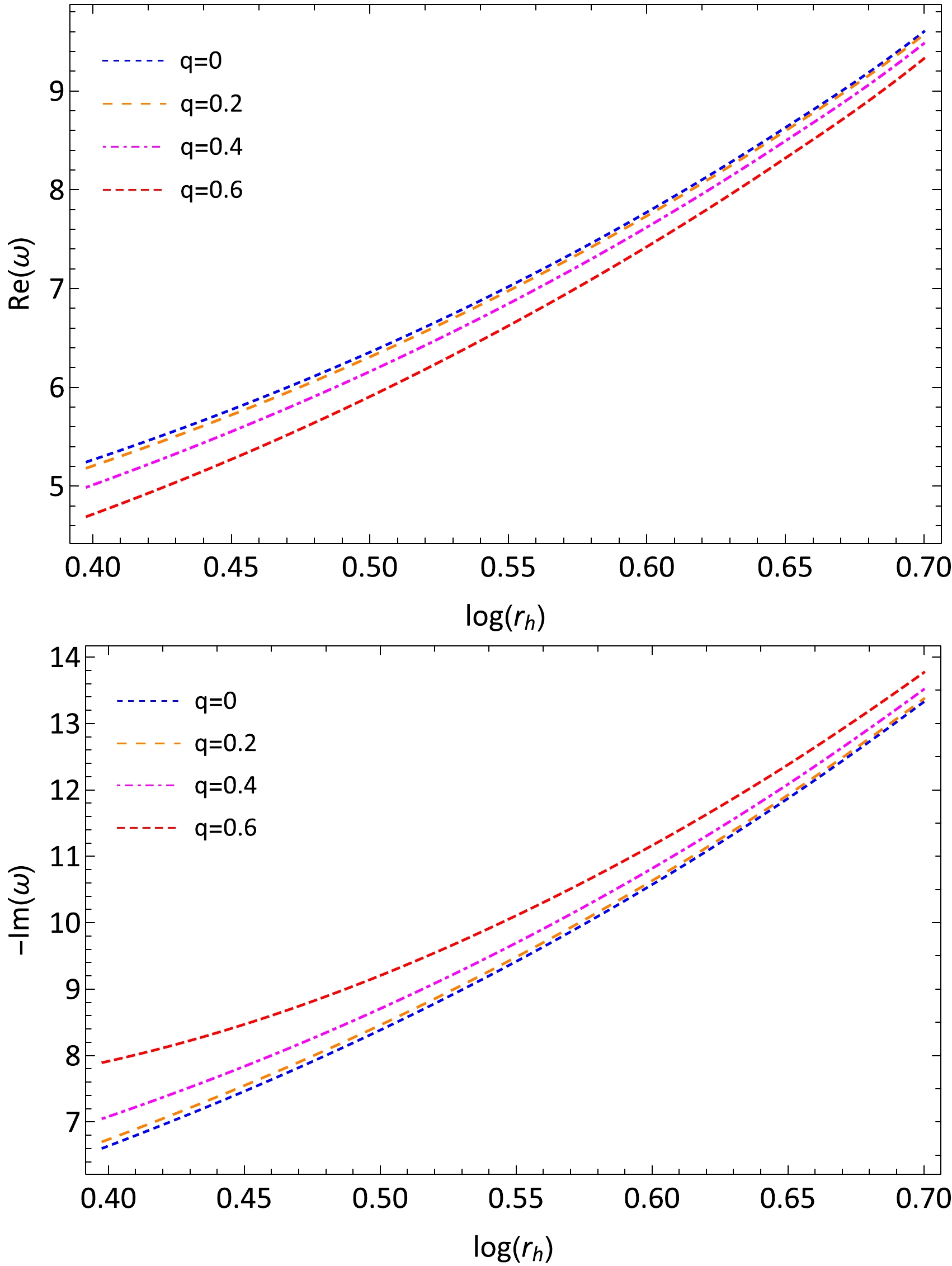

Figure 5.  (color online) QNM frequencies of the axial gravitational perturbation of the Bardeen Anti-de Sitter BHs with $ l=2 $ and $ n=1 $.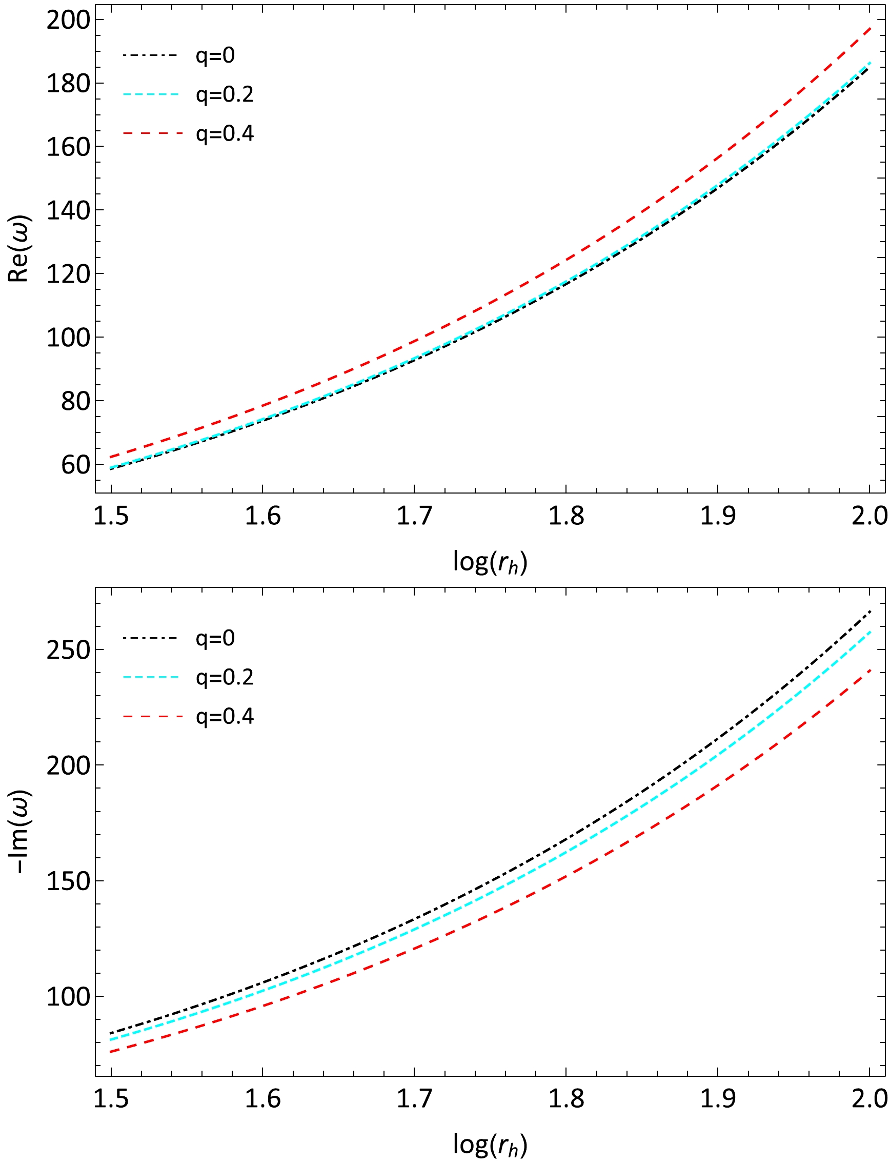

Figure 6.  (color online) QNM frequencies of the polar gravitational perturbation of the Bardeen Anti-de Sitter BHs with $ l=2,n=0 $.

In this study, we investigate the gravitational perturbations of the Bardeen BH in the presence of a cosmological constant. Both the axial (odd-parity) and polar (even-parity) sectors are considered, and we provide the detailed construction process for the decoupled equations with source terms. Then, we derive Schrödinger-type equations with effective potentials given by equations (25) and (29). Subsequently, we apply the WKB approach to analyze the quasinormal modes (QNMs) for the Bardeen de Sitter spacetime. The obtained QNM frequencies are presented in Tables 1 and 2. We explore various combinations of values for q and Λ while fixing l and n, and vice versa. The results reveal deviations between the QNM frequencies in the polar sector and those in the axial sector. We conduct additional calculations using different orders of q and the WKB approach to ensure that these deviations are not due to numerical errors, . Our findings demonstrate convergence, suggesting that the deviations are not due to the order of q or the WKB approach (and the currently used orders are sufficiently high to ensure the required accuracy of our conclusions). Moreover, numerical analysis indicates that the errors arising from different choices of the orders of q and the WKB approach are significantly smaller than the observed deviations. This provides evidence that the deviations are due to the inherent differences in odd and even parities rather than the order of q or the WKB approach.

The results unequivocally demonstrate that, for a fixed nonlinear electromagnetic charge q, the axial and polar gravitational perturbations exhibit distinct QNM frequencies. This observation indicates a violation of isospectrality in the case of Bardeen de Sitter BHs. Unlike linear electromagnetic fields, the presence of nonlinear electromagnetic fields disrupts the isospectrality of gravitational perturbations.

Furthermore, we compute the QNMs of the Bardeen Anti-de Sitter spacetime. To gain a clearer understanding of the impact of varying q on the QNMs, we consider different ranges for the parameter $ r_h $. Our results show the influence of the parameter q on the real and imaginary parts of the QNMs.

Notably, the master equations derived in this study contain source terms. However, owing to the QNM calculations in this study, we impose that the source terms vanish. However, if we consider the extreme mass ratio inspiral model, i.e., a point particle moving around the Bardeen BH, one can calculate the energy flux at infinity or the gravitational wave of inspiral phase using our master equations. In contrast, the Bardeen BH considered in this study is a simple RBH solution. The ABG solution seems to be a more reasonable choice as it approaches the Reissner-Nordström solution at asymptotic infinity [6]. Whether the breaking of isospectrality occurs in all nonlinear electromagnetic theories is worth further exploration. With the improvement of detection sensitivity, the LIGO/Virgo/KAGRA cooperation is expected to accurately measure the QNMs of the BH ringdown phase and confirm/deny the breaking of isospectrality from the QNM signal in the near future.

By projecting the perturbed metric $ h^{lm}_{ab} $ onto these orthogonal tensor bases, the expressions for coefficients A-K can be obtained.

Only the case of $ l\geq 2 $ is considered in this study.

The field equation of ${E}_{\rm A}-{E}_{\rm K}$

Here, we present the explicit expressions of the parameters in Eq. (23), which are given by

and the parameters appearing in the source term Eq. (24) are given by

Here, we have