Effects from hadronic structure of photon on $ {\boldsymbol B\boldsymbol\to\boldsymbol\phi\boldsymbol\gamma }$ and ${\boldsymbol B_{\boldsymbol s}\boldsymbol\to(\boldsymbol\rho^{\bf 0},\boldsymbol\omega)\gamma }$ decays

The B meson system, being a bound state that consists of a b quark and a light antiquark, provides an ideal laboratory for precise study of the Standard Model (SM) of particle physics and thus facilitates the search for new physics (NP). Because the b quark mass is much larger than the typical scale of the strong interaction, the otherwise troublesome long-distance strong interactions are generally less important and are under better control than in other lighter meson systems. Radiative decays $ B \to V \gamma $ are of particular interest in this respect. For example, the isospin-asymmetry parameter $ \Delta^{\pm0}=\Gamma(B^{\pm}\to\rho^{\pm}\gamma)/ [2\Gamma(B^0(\bar{B}^0)\to \rho^0\gamma)]-1 $ and the direct $ CP $ asymmetry parameter $\mathcal{A}_{CP}=[\mathcal{B}(B^-\to\rho^-\gamma)- \mathcal{B}(B^+\to\rho^+ \gamma)]/ [\mathcal{B}(B^-\to \rho^-\gamma) + \mathcal{B}(B^+\to\rho^+\gamma)]$ allow us to extract the angle α of the Cobibbo-Kobayashi-Maskawa (CKM) unitary triangle [1]. The radiative $ B\to K^*\gamma $ decays are usually viewed as probes of the NP [2, 3] because they are induced by the flavor-changing-neutral-current $ b\to s\gamma $that only occurs by loops. Therefore, it is meaningful to improve the theoretical predictions of these radiative decays, so as to match the accurate measurements to be obtained in the ongoing LHCb and Belle II experiments.

In the past few years, many efforts [4–8] have been devoted to improving the theoretical predictions of these exclusive radiative decays by including various corrections, such as next-to-leading order in the strong coupling $ \alpha_s $, non-factorizable corrections, and charm loop contributions. Each correction may affect the experimental observables, such as the branching fractions, $ CP $asymmetries, and forward-backward asymmetries. Some special radiative decays such as $ B\to\phi\gamma $ and $ B_s\to(\rho^0, \omega) \gamma $, where the quarks in the final state are different from those in the initial B meson, are called pure annihilation radiative decays. In particular, the annihilation diagrams are viewed as power suppressed by $ \Lambda/m_B $ with a typical hadronic scale Λ; therefore, the branching fractions are estimated to be small. For the decay $ B^0\to\phi\gamma $, which is induced by penguin operators, the decay amplitude can be factorized into the simple matrix $ \langle \phi|\bar s\gamma_\mu s|0\rangle $ and the transition form factor $ \langle \gamma|\bar{d}\gamma_{\mu}(1-\gamma_5)b|B^0\rangle $ in the naive factorization. Its branching fraction is estimated to be on the order of $ {\cal O}(10^{-13}) $, and it can be $ {\cal O}(10^{-12}) $ [9] by adding the QCD corrections. Within the perturbative QCD (PQCD) approach, its branching fraction has been predicted to be $ 1.6 \times10^{-12} $ [10] by one of us (Li). These predictions are still much smaller than the current available upper limit $ 1.0\times10^{-7} $ [11]. As a decay induced only by the penguin operators, the branching fraction might be enhanced remarkably by the effects of NP, such as in the R-parity violation supersymmetry model [9] and the non-universal $ Z^\prime $ model [12]. In this respect, before judging the effects of NP, we should calculate the branching fractions in the SM as precisely as possible.

As we know, in addition to the high order corrections of $ \alpha_s $, power corrections are important for the finite b quark mass. In the B meson decays, there are many types of power corrections, such as that from the high-twist distribution amplitudes of the B mesons [13–15], the high-twist light-cone distribution amplitudes (LCDAs) of the final state mesons [16, 17], and the hadronic structure of the photon (HSP) [18, 19] in radiative decays. In the framework of PQCD, the power corrections for $ B\to\gamma l \nu $ decay have also been investigated [19], wherein it was indicated that both the contribution from the high-twist B meson wave functions and the HSP can change the leading power result by approximately $ 20 $%. In view of the power counting rules, the corrections from high-twist LCDAs of light mesons are no more than $10$% for nonleptonic B decays [20]. For the radiative nonleptonic B decays that only occur through annihilation diagrams at leading power, when the HSP is considered, the contributions from emission diagrams are involved, and the branching ratio might be enhanced. Hence, the pure annihilation decays are perhaps sensitive to the power corrections. Motivated by this, we employ the PQCD approach to investigate the corrections from the HSP to the $ B\to\phi\gamma $ and $ B_s\to (\rho, \omega) \gamma $ amplitudes, so as to improve the precision of the theoretical prediction.

The outline of this paper is as follows. In Sec. II, we briefly review the theoretical background and summarize the expressions for the $ B\to\phi\gamma $ and $ B_s\to (\rho, \omega)\gamma $ amplitudes. In Sec. III, the numerical results and discussion are presented. We conclude this study in Sec. IV.

It is well known that, when facing annihilation type contributions, in collinear factorization such as QCD factorization, the singularities destroy the perturbative calculations, and then, parametrization is adopted to evaluate this type of contribution, which leads to a decrease in predictive ability. Using the PQCD approach [21, 22] based on $ k_T $ factorization, one can calculate the annihilation diagrams perturbatively, because the end-point singularities are smeared by keeping the intrinsic transverse momenta of the inner quarks. The pure annihilation decay $ B_s\to \pi\pi $ was first calculated in 2004 [23] and the predicted branching fraction was confirmed by LHCb in 2006 [24], which implies that the results of pure annihilation decays based on the PQCD approach are reliable.

In this study, we work in light-cone coordinates. In the B meson rest frame, the momenta of the initial B meson, the final vector meson (V), and the photon are expressed as

with $ r=m_V/m_B $, $ m_V $ and $ m_B $ being the masses of the vector meson and the B meson, respectively. For the light quark in the B meson, we denote its momentum as

where $ x_1 $ is the momentum fraction of the light quark, and $ \mathbf{k}_{1T} $ is the transverse momentum of the light quark. Similarly, the momentum of the quark of the final vector can be written as

In this study, we do not regard the photon as a point-like particle any more and consider its hadronic structure; then, the momentum of the light quark in the photon can be written as

In PQCD, the decay amplitude of the process $ B\to M_1M_2 $ is factorized into the convolution of the Wilson coefficients (WCs) $ C(t) $, the hard kernel $ H(x_i,b_i,t) $, and the wave functions of the initial and final states, which can be expressed as

with $ b_i $ being the conjugate variable of the transverse momentum $ k_{iT} $. The physics above the scale ($ m_b $) have already been absorbed into the WCs $ C(t) $. The hard kernel $ H(x_i,b_i,t) $ is governed by exchanging one hard gluon and can be calculated perturbatively. The parameter t is the largest scale appearing in the hard kernel $ H(x_i,b_i,t) $. The wave functions describing the soft physics below the factorization scale are not perturbatively calculable but universal, which can be studied in some nonperturbative approaches. The last exponential term is the so-called Sudakov form factor, which arises from the resummation on the double logarithmic terms containing the additional energy scale introduced by the transverse momentum.

In PQCD, the most important inputs are the wave functions, which describe the inner dynamics of the initial and final particles. In the past decades, the wave functions of the B meson and vector mesons have been well studied in two-body nonleptonic B decays, such as in Refs. [21–23, 25–28]. In general, the wave function $ \Phi_{M,\alpha\beta} $ with Dirac indices $ \alpha,\beta $ are decomposed into 16 independent components, $ 1_{\alpha\beta} $, $ \gamma^\mu_{\alpha\beta} $, $ \sigma^{\mu\nu}_{\alpha\beta} $, $ (\gamma^\mu\gamma_5)_{\alpha\beta} $, and $ \gamma_{5\alpha\beta} $. For the heavy pseudo-scalar B meson, the structure $ (\gamma^\mu\gamma_5)_{\alpha\beta} $ and $ \gamma_{5\alpha\beta} $ components remain as leading contributions. Therefore, $ \Phi_{B,\alpha\beta} $ is written as

where $ N_c = 3 $ is the color's degree of freedom, and $ \phi_B^{A,P} $ are Lorentz scalar wave functions. According to the heavy quark effective theory, we obtain $ \phi_B^P \simeq m_B \phi_B^A $. Hence, the B meson's wave function can be simplified as

For the Lorentz scalar wave function $ \phi_B(x,b) $, there is a sharp peak at the small x region; we use

which is adopted in Refs. [21, 22]. It is noted that $ \phi_B $ is normalized by the decay constant $ f_B $,

As mentioned above, the parameters $ \omega_b=0.40\pm0.08 $ for the$ B^0 $ meson and $ \omega_b=0.50\pm0.10 $ for the $ B^0_s $ meson are almost best fits from the well measured results of the $ B_{d,s}\to K\pi $, $ \pi \pi $ decays [21, 22, 28, 29], including the branching fractions and the $ CP $ asymmetries. For the vector mesons ϕ, $ \rho^0 $, and ω, we also pursue the same strategy and adopt the same wave functions obtained in QCD sum rules [30]. Very recently, the Gegenbauer moments in the wave functions of the light mesons have been fitted to available data of branching fractions and direct $ CP $ asymmetries globally [31], and the fitted results are in good agreement with those in [30].

When studying the hard exclusive processes involving photon emission in QCD, a specific feature is that a real photon contains both a pointlike, electromagnetic (EM) component and a soft, hadronic component. Similar to a transversely polarized vector meson, the two-particle distribution amplitudes of a final state photon can be defined as [32]

where λ and $ \varepsilon_\gamma $ denote the polarization and the related polarization vector. The Lorentz scalar wave functions $ \phi_\gamma(u,\mu) $ and $ \psi^{(a,v)}_\gamma(u,\mu) $ are twist-2 and twist-3 distribution amplitudes (DAs), respectively. $ \langle\bar q q\rangle $ and $ \chi(\mu) $ are the quark condensate and the corresponding magnetic susceptibility. $ f_{3\gamma} $ is the decay constant of the photon, which appears in the twist-3 DAs. It should be emphasized that $ \langle\bar q q\rangle $, $ \chi(\mu) $ and $ f_{3\gamma} $ are all scale dependent, and their evolution equations can be found in Refs. [18, 19]. Finally, we write the momentum space projector for the two-particle LCDAs (up to twist-3) as

and $ n=(1,0,{\bf 0}_T) $ and $ \bar n=(0,1,{\bf 0}_T) $ are two unit vectors with opposite directions. In our numerical calculations, the contributions from transverse momentum dependence of the photon wave functions are very small, which indicates that the last part in the third term can be neglected safely.

The distribution amplitudes $ \phi_{\gamma}(u,\mu) $, $ \psi^{v}(u,\mu) $ and $ \psi^{a}(u,\mu) $ have been systematically studied in Ref. [32], and their expressions are written as

with $ \xi=2u-1 $. $ C_n^{3/2}(\xi) $ and $ P_n(\xi) $ are Gegenbauer polynomials and Legendre polynomials, respectively. Since the scale dependence of the parameters $ b_n(\mu) $, $ \omega_{\gamma}^{V}(\mu) $ and $ \omega_{\gamma}^{A}(\mu) $ have been well studied in Refs. [19, 32], we do not show them here. Typically, when $\mu=1~ {\rm GeV}$, we have

Because the massless photon is transverse polarized only, the decay amplitude of the radiative decay $ B\to V\gamma $ can only be decomposed into two parts as

with the polarization vectors of the vector meson and the photon $ \varepsilon_V^* $ and $ \varepsilon_{\gamma}^* $, respectively. With the calculated $ \mathcal{A}^S $ and $ \mathcal{A}^P $ in the PQCD approach, the branching fraction of the $ B\to V\gamma $ decay is

where $ \tau_B $ is the lifetime of the B meson. At the leading order and the leading power, the decay amplitudes $ \mathcal{A}^S $ and $ \mathcal{A}^P $ have been calculated in detail in Ref. [10], and we do not present them further.

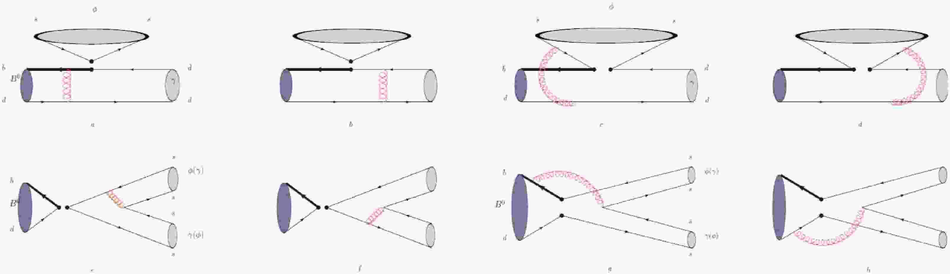
Now, we study the contributions from the HSP to decays $ B\to\phi\gamma $ and $ B_s\to(\rho^0,\omega)\gamma $. In the following, we take $ B^0\to \phi\gamma $ as an example for illustration, which is governed by the $ b\to d \bar s s $ transition. According to the effective Hamiltonian [33], the corresponding diagrams are plotted in Fig. 1. The decay amplitude with the contribution of the HSP can be expressed as

Figure 1.  (color online) Leading order Feynman diagrams of $B^0\to \phi \gamma$ decay with the hadronic structure of the photon in PQCD.

with $ i=S,P $. The combined coefficients $ a_i $ are defined as

The subscripts "$ ef $" and "$ enf $" stand for the factorizable and nonfactorizable diagrams with the emission of a ϕ meson, respectively. Similarly, "$ af1(2) $" and "$ anf1(2) $" mean the factorizable and nonfactorizable annihilation diagrams, where the number "1 (2)" means the case in which the produced strange quark enters the ϕ meson (γ). The superscripts "$ LL $," "$ LR $," and "$ SP $" represent the inserted $ (V-A)\otimes(V-A) $, $ (V-A)\otimes (V+A) $, and $(S-P)\otimes (S+P)$ currents. The expressions of the diagrams with different operators are given in the Appendix. Combining Eqs. (19) and (20), we calculate the branching fraction of this decay.

In this section, we first list some parameters in our numerical calculations as [11, 30]

Using the above input parameters, we calculate the branching fractions of $ B^0 \to \phi \gamma $,$ B_s \to \rho^0\gamma $, and $ B_s \to \omega\gamma $ including corrections from the HSP at leading order and list the results in Table 1. In addition, the results of the leading power are presented for comparison. In our calculations, three types of errors have been studied, which are from uncertainties of the nonperturbative physics, unknown QCD corrections, and CKM matrix parameters. The first errors are from the uncertainties of the parameters in the wave functions, such as the decay constants and the inner parameters in the distribution amplitudes of the initial and final mesons. It should be emphasized that these types of errors are dominant, and more precise results from nonperturbative approaches are needed in future. The second uncertainty comes from the QCD scale $\Lambda_{\rm QCD}$ and the hard kernel scale t, whose variants reflect the effects of the higher order QCD corrections. In this study, we set $\Lambda_{\rm QCD}=(0.25\pm 0.05)~{\rm GeV}$ and vary t from $ 0.8t $ to $ 1.2t $. The final errors are caused by the CKM matrix elements.

Decay modes	LO($ 10^{-12} $)	IBR($ 10^{-11} $)
$ B^0 \to \phi \gamma $	$ 0.9^{+0.2+0.3+0.0}_{-0.2-0.4-0.0} $	$ 3.57^{+2.12+0.25+0.19}_{-1.58-0.31-0.14} $
$ B_s \to \rho^0 \gamma $	$ 72.8^{+26.5+4.6+2.4}_{-21.0-4.4-3.3} $	$ 12.4_{-3.87-0.55-0.60}^{+4.98+1.04+0.70} $
$ B_s \to \omega\gamma $	$ 8.6^{+5.3+6.9+0.2}_{-3.4-4.2-0.2} $	$ 35.1_{-21.2-4.14-1.90}^{+31.8+2.13+1.70} $

Table 1.  Leading order (LO) branching ratios and improved branching ratios (IBR) of the pure annihilation type $ B\to V\gamma $ decays in the PQCD approach.

From Table 1, one finds that, at the leading order, the branching fractions of the $ B_s\to (\rho^0,\omega)\gamma $ decays are much larger than that of $ B^0\to\phi\gamma $; this is because the former decays have the $ \bar uu $component and thus gain contributions from the tree operators with larger WCs. It is important to note that, when the contributions from HSP are included, the branching fractions of all concerned decays are enhanced remarkably, and the branching fraction of $ B\to \phi\gamma $ increases by approximately 40 times compared with that of leading power. At leading power,$ B\to \phi\gamma $ is governed by the transition $ b\to d \bar s s $, and the produced $ \bar s $ and s quarks form the final ϕ meson. The photon can be radiated from any quark participating in the weak interaction. Due to the symmetry, the contributions of the photon radiated from the strange and anti-strange quarks are canceled by each other; therefore, only the diagrams with photons emitted from the beauty and down quarks contribute to the amplitudes. The explicit amplitudes are given in Ref. [10]. When the contributions of the HSP are included, more diagrams contribute to the amplitudes $ \mathcal{A}^S $ and $ \mathcal{A}^P $, as shown in Fig. 1. Compared with diagrams of leading power, both factorizable and nonfactorizable emission diagrams contribute to the amplitudes without cancellations. Furthermore, for the nanfactorizable diagrams, besides the $ (V-A)(V-A) $ operators, the $ (S-P)(S+P) $ operator that results from the Fierz transformation of the $ (V-A)(V+A) $ takes large contributions. This picture is very similar to that of the $ B \to \rho^0\phi $ decay. After summing all contributions, we find that the amplitude from the HSP is much larger than that of the leading power, leading to a larger branching fraction.

Generally, the power expansion ($ 1/m_B $) in B meson decays is an effective expansion in most decay modes, such as two-body non-leptonic decays. As stated in Sec. I, there are many sources of power corrections, such as the high-twist DAs of B and light mesons, the soft corrections to the leading twist contributions, and the subleading power “hadronic” photon correction. For the power corrections from B and light mesons, their contributions are less than $ 20 $%. Such corrections could be plagued by large theoretical uncertainties, and we have not discussed these effects yet in the current work. However, for the pure annihilation radiative $ B\to V\gamma $ decays, the leading power contributions (annihilation diagrams) are already power suppressed compared with decays dominated by the emission type diagrams. When the HSP is taken into account, the emission diagrams are involved, which enhances the next-to-leading power contributions and makes the higher power corrections significantly larger than those of the leading power. All these can be summarized as follows: for some special decay modes, if the leading power contributions are suppressed by some mechanism, the higher power contributions could be larger than those of the leading power, which may lead to the branching fraction being enhanced significantly.

We also note that the branching fractions of $ B_s \to \rho^0\gamma $ and $ B_s \to \omega\gamma $ are on the order of $ {\cal O}(10^{-10}) $, and that of $ B \to \phi\gamma $ is on the order of $ {\cal O}(10^{-11}) $. Unfortunately, such small branching fractions cannot be measured in current experiments. To highlight the effects of the corrections from HSP, we define a ratio as follows:

which can reduce of the dependence on the nonperturbative parameters effectively. At leading power, $ \mathcal{R}_{\rho\omega}\sim 8 $ is much larger than 1, whereas this ratio becomes 0.35 when the HSP is involved. It is apparent that this ratio decreases by approximately 40 times; thus, it may be a good probe for testing the effects of HSP when the data are available. At leading order, because of the interference between the$ u\bar{u} $ and $ d\bar{d} $ components, $ B_s \to \rho^0\gamma $ has larger penguin contributions than $ B_s \to \omega\gamma $, leading to the branching fractions of $ B_s \to \rho^0\gamma $ being much larger than that of $ B_s \to \omega\gamma $. When including the HSP corrections, although they are suppressed by the CKM matrix elements and the power, the newly introduced tree contributions by the $ \bar u u $ component in the photon are comparable with those of penguin contributions, due to the large WCs, especially in the nonfactorizable diagrams. Because the signs of $ \bar dd $ in $ \rho^0 $ and ω are different, the interferences between contributions of tree operators and penguin ones are different for $ B_s \to \rho^0\gamma $ and $ B_s \to \omega\gamma $ decays. Again, due to the interference between the tree and penguin contributions, the HSP corrections to $ B_s\to\rho^0\gamma $ are much smaller than those to $ B_s\to\omega\gamma $, leading to a small $ R_{\rho\omega} $.

As mentioned above, the HSP corrections could increase the branching fractions of these pure annihilation decays remarkably. In Ref. [19], it is found that the contribution of the HSP plays an important role in the $ B\to\gamma l \nu $ decay and the branching faction can be decreased by $20$%. In Ref. [34], the contributions of electromagnetic penguin operators to $ B_s\to (\rho^0,\omega)\gamma $ decays have also been examined in QCDF, and the results indicate that they are suppressed by the electromagnetic coupling constant $ \alpha_e $. Very recently, these three decays have been comprehensively analyzed at leading power in the framework of soft-collinear effective theory in [35], where the authors found that the $ \phi-\omega-\rho^0 $ mixing effect could enhance the branching fractions of $ B^0 \to \phi\gamma $ and $ B_s\to \omega \gamma $ by approximately three orders of magnitude. If their conclusion holds in PQCD, the branching fractions of $ B^0 \to \phi\gamma $ and $ B_s\to \omega\gamma $ are roughly estimated to be on the order of $ 10^{-8} $ and $ 10^{-7} $, respectively, which might be measurable in Belle-II and LHCb experiments. Future measurements on these decays will be helpful in discerning all the above physics mechanisms.

As pure annihilation type radiative B decays suppressed by $ \Lambda/m_B $, the decays $ B\to\phi\gamma $ and $ B_s\to(\rho^0,\omega)\gamma $ governed by flavor changing neutral currents have small branching fractions, which makes them very sensitive to the effects of the new physics beyond the SM. Before studying the effects of new physics, it is necessary for us to calculate the observables in the SM with high precision. In this study, we mainly investigate the power corrections from the HSP in these pure annihilation decays. Because the quark components in photons are taken in account, emission diagrams are involved, which are not suppressed in comparison to the annihilation diagrams. Thus, the branching fraction of $ B\to \phi\gamma $ is enhanced by approximately 40 times, and the branching fractions of $ B_s \to \rho^0\gamma $ and $ B_s \to \omega\gamma $ are on the order of $ {\cal O}(10^{-10}) $. Moreover, to shed light on these types of corrections and reduce theoretical uncertainties, we define a ratio of branching fractions of $ B_s \to \rho^0\gamma $ and $ B_s \to \omega\gamma $, namely $ \mathcal{R}_{\rho\omega} $, and find that this ratio is changed significantly by the HSP. All the above results can be tested in high luminosity accelerators in the future.

The amplitudes of factorizable emission diagrams (a and b) with the $ (V-A)(V-A) $ current are given as

with the color factor $ C_F=4/3 $ and the $ \phi(1020) $ meson decay constant $ f_{\phi}^T $. $ Q_d $ is the charge of the down quark in the hadronic structure of the photon. The Sudakov form factors $ E_{ef} $, hard functions $ h_{ef} $, and scales $ t_{a,b} $ can be found in Ref. [27] because the behaviors of the photon are very similar to a vector.

For the nonfactorizable emission diagrams (c and d), not only the $ (V-A)(V-A) $ current but also the $ (S-P)(S+P) $ current can be inserted, and the corresponding amplitudes are written as

For the annihilation diagrams (e-h), because the produced strange quark can enter not only the ϕ meson but also the photon, we have to discuss two cases. If the strange quark enters the photon, the corresponding factorizable and nonfactorizable annihilation amplitudes with possible currents are given as

When the strange quark enters the ϕ meson, the amplitudes are expressed as