


 Abstract
 HTML
HTML Reference
 Related
 PDF
PDF


-
The image of the M87* supermassive black hole captured by the Event Horizon Telescope (EHT) Collaboration in 2019 indicated a crucial new avenue to probe black holes through electromagnetic signals. The black hole image and its inner shadow carry essential information on the hair, such as mass, electric charge, and angular momentum, that characterizes the black hole [1]. The measurements are performed in terms of the electromagnetic signals, largely dictated by the strong gravitational lensing. The classical geometric-optics limit [2–4] of the electromagnetic waves, referred to as photons, follow the null geodesics of the black hole metric in question. The latter can be derived by analyzing the wavefront propagation at the high frequency limit by treating the amplitude variation as an insignificant quantity. In this regard, light propagation in nonlinear electrodynamics (NLED) is a notable topic, as it presents intriguing features distinct from classical electrodynamics. In particular, in the NLED environment, photons do not propagate along the null geodesics of the background geometry. Instead, they traverse the media in accordance with an effective geometry [5] related to the specific form of the NLED Lagrangian.
In recent decades, many modifications of Einstein's gravitational theory that involve NLED have been proposed, among which the Born-Infeld (BI) theory of gravity [6–8] has aroused much attention. Hoffmann, Infeld, and Perez [9, 10] developed the first black hole solution coupled to a nonlinear electromagnetic field that gives rise to an exact solution to the Einstein Born-Infeld (EBI) theory. Other studies [11–14] have indicated that some difficulties in general relativity can be partly resolved by coupling logarithmic or exponential NLED to the gravity sector. In addition, by studying the charged static black hole solutions in the presence of NLED, it was concluded that the latter has a sizable impact on the properties of black holes [15–19].
Dictated by strong gravitational lensing, in general relativity, the trajectory of a photon is significantly deflected in the vicinity of massive compact objects. For light beams that pass near a black hole, only the geodesics that eventually arrive at an observer's field of view, specified by its celestial coordinates, can be observed. At the other end of the geodesic, if it escapes to infinity, it corresponds to a bright pixel in celestial coordinates. In contrast, if the photon falls into the black hole's horizon, it potentially corresponds to a dark spot. Subsequently, as a silhouette, the black hole shadow is defined as the innermost boundary of the collection of bright pixels (but conceptually, not the outmost boundary of the union of dark spots). In practice, the black hole shadow can be identified by exploring the fundamental photon orbits [20–23]. By studying black hole shadows, one is expected to learn about the physics of the black hole itself and the spacetime structure near the black hole. In the context of NLED, the photon's trajectory is governed by the propagation of the discontinuity in the waveform [5]. In this regard, the study of shadows of black holes in NLED may provide crucial information on the properties of nonlinear electrodynamic fields, which find many implications in modern physics. The present study is motivated by the above considerations and explores black hole shadows associated with logarithmic and exponential nonlinear electrodynamic models for slowly rotating black holes in anti-de Sitter spacetime [16]. The effective geometries are derived, and the resulting black hole images and shadows are investigated. In addition, we also discuss the impact of different metric parameters, particularly the NLED coupling, on the properties of black hole shadows.
The remainder of the paper is organized as follows. In Sec. II, we briefly review the slowly rotating black hole in logarithmic NLED and calculate the effective metric. In Sec. III, the resulting black hole shadows are obtained by numerical ray-tracing simulations. The effects of different metric parameters, such as spin, charge, and nonlinear coupling, on the black hole shadows are elaborated. In Sec. IV, we explore the case of exponential NLED for slowly rotating black holes. Further discussions and concluding remarks are given in the last section.
-
In this study, we consider the Einstein–Hilbert action with a negative cosmological constant Λ, minimally coupled to the NLED. The Lagrangian is expressed as follows:
$ \begin{array}{*{20}{l}} \mathcal{L}=R-2{\Lambda}+L(F), \end{array} $

(1) where R is the Ricci scalar, and
$ L(F) $ possesses a logarithmic form [24],$ L(F)=-8{\beta}^2\ln\left(1+\frac{F}{8{\beta}^2}\right), $

(2) where β measures the nonlinear coupling, and
$ F=F_{\mu\nu}F^{\mu\nu} $ is the Maxwell invariant, where$ F_{\mu\nu} $ is the electromagnetic tensor defined by$ F_{\mu\nu}=\partial_\mu A_\nu-\partial_\nu A_\mu $ .In NLED theory, the static equation is rather complex, and as a result, it is not straightforward to derive a rotational solution from the static one. Nonetheless, the formalism becomes manageable if one considers the slow rotation limit. In previous studies [25–28], some authors employed the perturbation theory by taking the spin parameter as the expansion parameter. Subsequently, the linear order equation of motion was derived, and the rotational black hole solution was obtained. For the present study, we consider the following slowly rotating charged black hole solution [24]:
$ \begin{aligned}[b] {\rm d}s^2=&-G(r){\rm d}t^2+\frac{{\rm d}r^2}{G(r)}-2aG(r)\cos\theta {\rm d}t{\rm d}{\phi}+r^2{\rm d}{\theta}^2\\&+r^2\sin^2{\theta}{\rm d}{\phi}^2,\\ G(r)=&1-\frac{2M}{r}-\frac{\Lambda r^2}{3}+\frac{8\beta^2r^2}{3}-\frac{4q^2}{r}\int{\frac{{\rm d}r}{r^2(\Gamma-1)}}\\&-\frac{4\beta^2}{r}\int{r^2\ln\left(\frac{2}{\Gamma+1}\right){\rm d}r}, \end{aligned} $

(3) where
$ G(r) $ is already known in Einstein-Maxwell gravity with$ \Gamma=\sqrt{1+\left(\dfrac{q^2}{\beta^2r^4}\right)} $ , a is the spin parameter, M gives the black hole mass, and q is related to electric charge.The one-form electromagnetic potential is given by
$ \begin{array}{*{20}{l}} A=h(r)[{\rm d}t+a\cos\theta {\rm d}\phi], \end{array} $

(4) where
$ h'(r)=\frac{2q}{r^2(\Gamma+1)}, $

(5) where the prime indicates the first-order derivative with respect to r.
Using Eq. (4), one obtains the explicit forms of the non-vanishing components of the electromagnetic tensor
$ F_{\mu\nu} $ as follows:$ \begin{aligned}[b] F_{tr}=&-F_{rt}= -h'(r),\\ F_{r\phi}=&-F_{\phi r}= a\cos\theta h'(r),\\ F_{\theta \phi}=&-F_{\phi \theta}= -ah(r)\sin\theta . \end{aligned} $

(6) -
As mentioned before, a photon's trajectory in the NLED medium is not governed by the null-geodesic of the background matric. Instead, it propagates along the null-geodesic of an effective geometry [5]. Such an effective geometry has been employed to study the trajectory of light beams in black hole shadows in several studies, such as [29, 30]. In this section, we study the motion of photons in a slowly rotating charged black hole background given by Eq. (3). Following Novello et al. [5], the trajectory of the photon is governed by the propagation of discontinuity in the first-order derivation of the electromagnetic field, which occurs in the direction of the wave vector. To be specific, the propagation vector
$ k^{\mu} $ satisfies the following equation:$ \begin{array}{*{20}{l}} { } (L_{F}\hat{g}^{\mu\nu}-4L_{FF}F^{\mu\alpha}F_{\alpha}^{\nu})k_{\mu}k_{\nu}=0, \end{array} $

(7) where
$ \hat{g}^{\mu\nu} $ is the metric of the spacetime,$ L_F\equiv\dfrac{\partial L}{\partial F} $ and$ L_{FF}\equiv\dfrac{\partial^2 L}{\partial F^2} $ . From Eq. (7), one can readily extract an effective spacetime metric$ g^{\mu\nu} $ (without "hat") that reads$ \begin{array}{*{20}{l}} { } g^{\mu\nu}=L_F \hat{g}^{\mu\nu}-4L_{FF}F^{\mu}_{\alpha}F^{\alpha\nu} . \end{array} $

(8) Besides the fact that
$ k^{\mu} $ is a null vector in the effective metric, it can be shown that it propagates along the geodesic governed by Eq. (8).Using the non-vanishing metric components given by Eq. (3) and Eq. (8), we obtain the effective metric of the logarithmic NLED model,
$ \begin{array}{*{20}{l}} {\rm d}s^2=g_{tt}{\rm d}t^2+g_{rr}{\rm d}r^2+g_{\theta\theta}{\rm d}{\theta}^2+g_{\phi\phi}{\rm d}{\phi}^2+2g_{t\phi}{\rm d}t{\rm d}{\phi}, \end{array} $

where
$ \begin{aligned}[b] g_{tt}=&\frac{8q^4+30q^2r^4\beta^2-10r^5\beta^2(6M-3r+\Lambda r^3)}{15r^2\Bigg(q^2+r^4\beta^2\Bigg(1+\sqrt{1+\dfrac{q^2}{r^4\beta^2}}\Bigg)\Bigg)},\\ g_{rr}=&\frac{30r^{10}\beta^4}{\Bigg(q^2+r^4\beta^2\Bigg(1+\sqrt{1+\dfrac{q^2}{r^4\beta^2}}\Bigg)\Bigg)(-4q^4-15q^2r^4\beta^2+5r^5\beta^2(6M-3r+\Lambda r^3))},\\ g_{\theta\theta}=&-\frac{2r^2}{1+\sqrt{1+\dfrac{q^2}{r^4\beta^2}}},\\ g_{\phi\phi}=&-\frac{2r^2\sin^2{\theta}}{1+\sqrt{1+\dfrac{q^2}{r^4\beta^2}}},\\ g_{t\phi}=&\frac{2a \cos{\theta}(4q^4+15q^2r^4\beta^2-5r^5\beta^2(6M-3r+\Lambda r^3))}{15r^2\Bigg(q^2+r^4\beta^2\Bigg(1+\sqrt{1+\dfrac{q^2}{r^4\beta^2}}\Bigg)\Bigg)}. \end{aligned} $ 
(9) Due to the hypergeometric functions, we note that these quantities are second-order in q.
The horizons associated with NLED perturbations are given by
$ (g_{rr})^{-1}=0 $ , and one finds$ \begin{array}{*{20}{l}} -4q^4-15q^2r^4\beta^2+5r^5\beta^2(6M-3r+\Lambda r^3)=0. \end{array} $

(10) It is noted that the radius obtained above is related to the propagation of discontinuity in NLED but not necessarily to other types of perturbations. Moreover, it is a function of the nonlinear coupling β. In the remainder of the paper, the word "horizon" refers to the propagation of quanta of NLED and, therefore, the light rings and black hole shadows.
-
In this section, we study the images of the charged, slowly rotating black holes using backward ray tracing [31]. The motion of the photon is described by the Lagrangian
$ L=\frac{1}{2}g_{\mu\nu}\dot{x}^{\mu}\dot{x}^{\nu} , $

(11) where the dot represents the derivative with respect to the affine parameter.
There are two killing vectors
$ \zeta_t $ and$ \zeta_{\phi} $ , related to the time and azimuthal angle translational invariance of the effective metric Eq. (8). In other words, the metric components are independent of t and ϕ, so one has two constants of integration, namely, the energy and angular momentum:$ -P_t=-\frac{\partial{L}}{\partial{\dot{t}}}=-g_{tt}\dot{t}-g_{t\phi}\dot{\phi}\equiv E, $

(12) $ +P_{\phi}=\frac{\partial{L}}{\partial{\dot{\phi}}}=g_{\phi\phi}\dot{\phi}+g_{t\phi}\dot{t}\equiv L_z , $

(13) where E is the energy of the moving photon, and
$ L_z $ corresponds to the z component of angular momentum.In terms of the two conserved quantities, we obtain the motion equation for a photon along a null-geodesic:
$ \begin{aligned}[b] \ddot{r}=&\frac{1}{2}g^{rr}\Bigg[\Bigg(\frac{\partial{g_{tt}}}{\partial{r}}\Bigg)\dot{t}^2+2\Bigg(\frac{\partial{g_{t\phi}}}{\partial{r}}\Bigg)\dot{t}\dot{\phi}+\Bigg(\frac{\partial{g_{\phi\phi}}}{\partial{r}}\Bigg)\dot{\phi}^2\\&-\Bigg(\frac{\partial{g_{rr}}}{\partial{r}}\Bigg)\dot{t}^2-2\Bigg(\frac{\partial{g_{rr}}}{\partial{\theta}}\Bigg)\dot{r}\dot{\theta}+\Bigg(\frac{\partial{g_{\theta\theta}}}{\partial{r}}\Bigg)\dot{\theta}^2\Bigg],\\ \end{aligned} $

$ \begin{aligned}[b] \ddot{\theta}=&\frac{1}{2}g^{\theta\theta}\Bigg[\Bigg(\frac{\partial{g_{tt}}}{\partial{\theta}}\Bigg)\dot{t}^2+2\Bigg(\frac{\partial{g_{t\phi}}}{\partial{\theta}}\Bigg)\dot{t}\dot{\phi}+\Bigg(\frac{\partial{g_{\phi\phi}}}{\partial{\theta}}\Bigg)\dot{\phi}^2\\&+\Bigg(\frac{\partial{g_{rr}}}{\partial{\theta}}\Bigg)\dot{r}^2-2\Bigg(\frac{\partial{g_{\theta\theta}}}{\partial{r}}\Bigg)\dot{r}\dot{\theta}-\Bigg(\frac{\partial{g_{\theta\theta}}}{\partial{\theta}}\Bigg)\dot{\theta}^2\Bigg],\\ \dot{t}=&\frac{Eg_{\phi\phi}+L_{z}g_{t\phi}}{g_{t\phi}^2-g_{tt}g_{\phi\phi}},\\ \dot{\phi}=&\frac{Eg_{t\phi}+L_{z}g_{tt}}{g_{tt}g_{\phi\phi}-g_{t\phi}^2}. \end{aligned} $

(14) Eq. (14) is then solved by numerical integration.
In order to evaluate the celestial coordinate, one makes use of the relation
$ {e_{\hat{\mu}}}={e_{\hat{\mu}}^{\nu}}\partial_{\nu} $ to transform the observer basis ($ {e_{\hat{t}}} $ ,$ {e_{\hat{r}}} $ ,$ {e_{\hat{\theta}}} $ ,$ {e_{\hat{\phi}}} $ ) into the coordinate basis ($ \partial_{t} $ ,$ \partial_{r} $ ,$ \partial_{\theta} $ ,$ \partial_{\phi} $ ) in a Zero-Angular-Moment-Observers (ZAMOs) reference frame. The transform matrix$ {e_{\hat{\mu}}^{\nu}} $ follows$ g_{\mu\nu}{e_{\hat{\alpha}}^{\nu}}{e_{\hat{\beta}}^{\nu}}=\eta_{\hat{\alpha}\hat{\beta}} $ , where$ \eta_{\hat{\alpha}\hat{\beta}} $ is the metric of flat spacetime. For the model we are studying, the transform matrix possesses the following form:$ \begin{array}{*{20}{l}} {e_{\hat{\mu}}^{\nu}}= \left[{\begin{array}{cccc} \zeta&0&0&\gamma\\ 0&A^r&0&0\\ 0&0&A^{\theta}&0\\ 0&0&0&A^{\phi}\\ \end{array}}\right], \end{array} $

(15) where ζ, γ,
$ A^r $ ,$ A^{\theta} $ , and$ A^{\phi} $ are real coefficients. By the normalization$ {e_{\hat{\mu}}}{e^{\hat{\nu}}}={\delta_{\hat{\mu}}}^{\hat{\nu}} $ , one has$ \begin{aligned}[b] A^r=&\frac{1}{\sqrt{g_{rr}}},\;\; A^{\theta}=\frac{1}{\sqrt{g_{\theta\theta}}},\;\; A^{\phi}=\frac{1}{\sqrt{g_{\phi\phi}}}, \end{aligned} $

$ \begin{aligned}[b] {\zeta}=&\sqrt{\frac{g_{\phi\phi}}{g_{t \phi}^2-g_{tt} g_{\phi\phi}}},\;\; \gamma=-\frac{g_{t \phi}}{g_{\phi\phi}}\sqrt{\frac{g_{\phi\phi}}{g_{t \phi}^2-g_{tt} g_{\phi\phi}}}. \end{aligned} $

By projecting a photon's four momentum
$ p^{\mu} $ onto the observer coordinate base$ e_{\hat{\mu}} $ , we can obtain the corresponding local four momentum$ p^{\hat{\mu}} $ $ \begin{array}{*{20}{l}} p^{\hat{t}}=-p_{\hat{t}}=-{e_{\hat{t}}}^{\nu}p_{\nu},~~ p^{\hat{i}}=p_{\hat{i}}={e_{\hat{i}}}^{\nu}p_{\nu}. \end{array} $

(16) The components can be further simplied to read
$ \begin{aligned}[b] p^{\hat{t}}=&\zeta E-\gamma L,\quad p^{\hat{r}}=\frac{1}{\sqrt{g_{rr}}}p_r,\\ p^{\hat{\theta}}=&\dfrac{1}{\sqrt{g_{\theta\theta}}}p_\theta,\quad p^{\hat{\phi}}=\frac{1}{\sqrt{g_{\phi\phi}}}L. \end{aligned} $

Subsequently, the celestial coordinates of a received photon, from the observer's perspective, can be readily expressed as [32]
$ \begin{aligned}[b] x=&-r\frac{p^{\hat \phi}}{p^{\hat r}}\bigg|_{(r_\mathrm{obs},\theta_\mathrm{obs})}=-\frac{r_\mathrm{obs}L_z}{\sqrt{g_{rr}}\sqrt{g_{\phi\phi}}\dot{r}},\\ y=&r\frac{p^{\hat \theta}}{p^{\hat r}}\bigg|_{(r_\mathrm{obs},\theta_\mathrm{obs})}=\frac{r_\mathrm{obs}\dot{\theta}\sqrt{g_{\theta\theta}}}{\dot{r}\sqrt{g_{rr}}}. \end{aligned} $

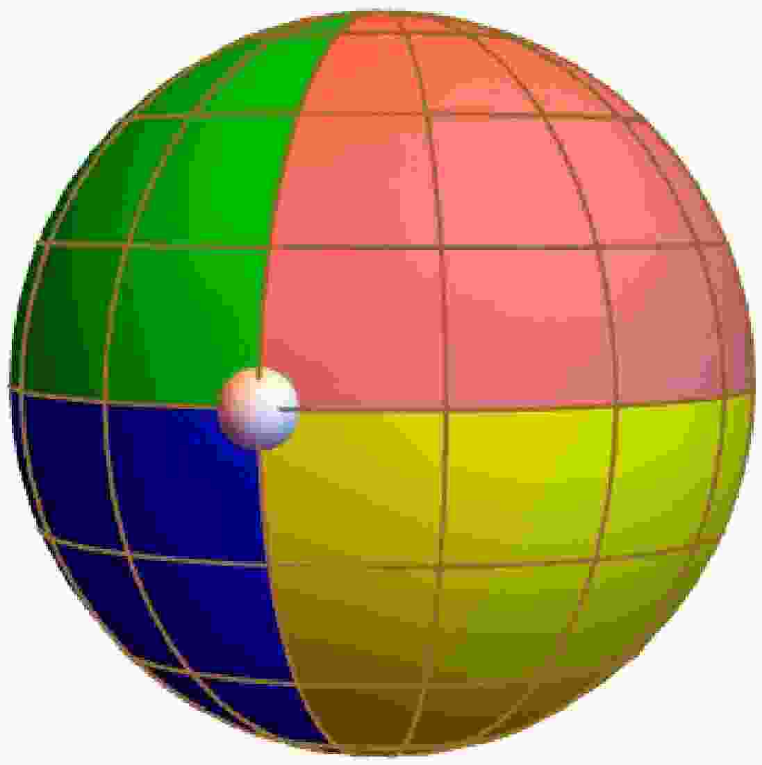
(17) In practice, we backwardly track the photons, from the observer's perspective, by considering their motions in the opposite direction of time. To be specific, a photon is effectively emitted from the observer, and it either ends up at the celestial sphere or falls into the black hole horizon. Following [33–38], we divide the celestial sphere into four color-coded quadrants. As shown in Fig. 1, the colors of the four quadrants are green, pink, blue, and yellow. Brown is used to mark the warp and weft. For convenience, we place the observer at the intersection of the four quadrants of the celestial sphere (not shown in Fig. 1), and therefore, we have
$ r_\mathrm{obs}=r_\mathrm{sphere} $ . The white dot shown in Fig. 1 is located at another intersection of the four-color quadrant, precisely opposite to the observer. In practice, it contributes primarily to the (first) Einstein ring. Based on the above configurations, the image of the black hole is then generated by integrating null geodesics emanated from the observer. If it falls into the horizon, it is marked as a black pixel. Roughly speaking, the collection of the black pixels forms the black hole shadow. Otherwise, a color is assigned to the pixel according to its specific location on the celestial sphere. In our study, the position of the observer is chosen to be$ r_\mathrm{obs} = 50M $ with the inclination angle$ \theta_\mathrm{obs} = 90^{\circ} $ .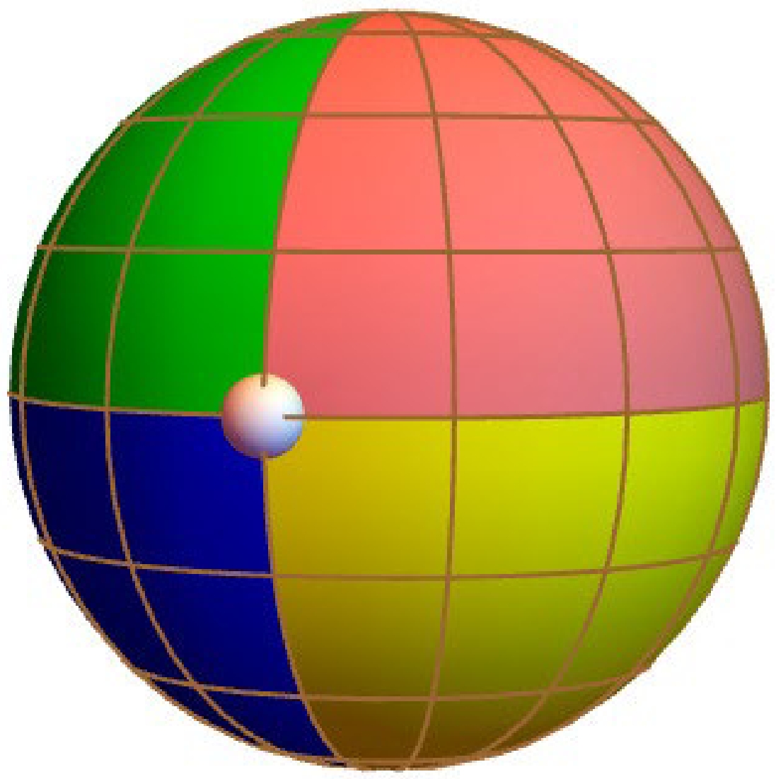
Figure 1. (color online) Painted celestial sphere. The colors assigned to different solid angles are visualized by the observer in their local celestial coordinates, obtained by numerical calculaions.
In what follows, we present the resulting black hole image and shadow obtained by numerical simulations. Then, we investigate the impact of different spin parameters a, charge q, and nonlinear coupling β on the size and shape of the black hole. We divide our discussions of the black hole image into three subsections.
-
In Fig. 2, we present the image and shadow cast by slowly rotating black holes for different spin parameters a. Here, we have chosen the parameters
$ M=2 $ ,$ q=1 $ , Λ= –1, and$ \beta=1 $ . The white dot on the celestial sphere turns into the (visually feasible, the first) Einstein ring due to the strong gravitational lensing. The effect is particularly apparent for the static black hole with$ a=0 $ , shown in the top-left plot of Fig. 2. The region inside the Einstein ring corresponds to photons that are deflected more than those associated with the Einstein ring. This implies that these photons must enter from the opposite side and travel for at least an additional half circle to reach the observer. This, in turn, explains why the colors of the image are inverted (for integer times) inside the ring.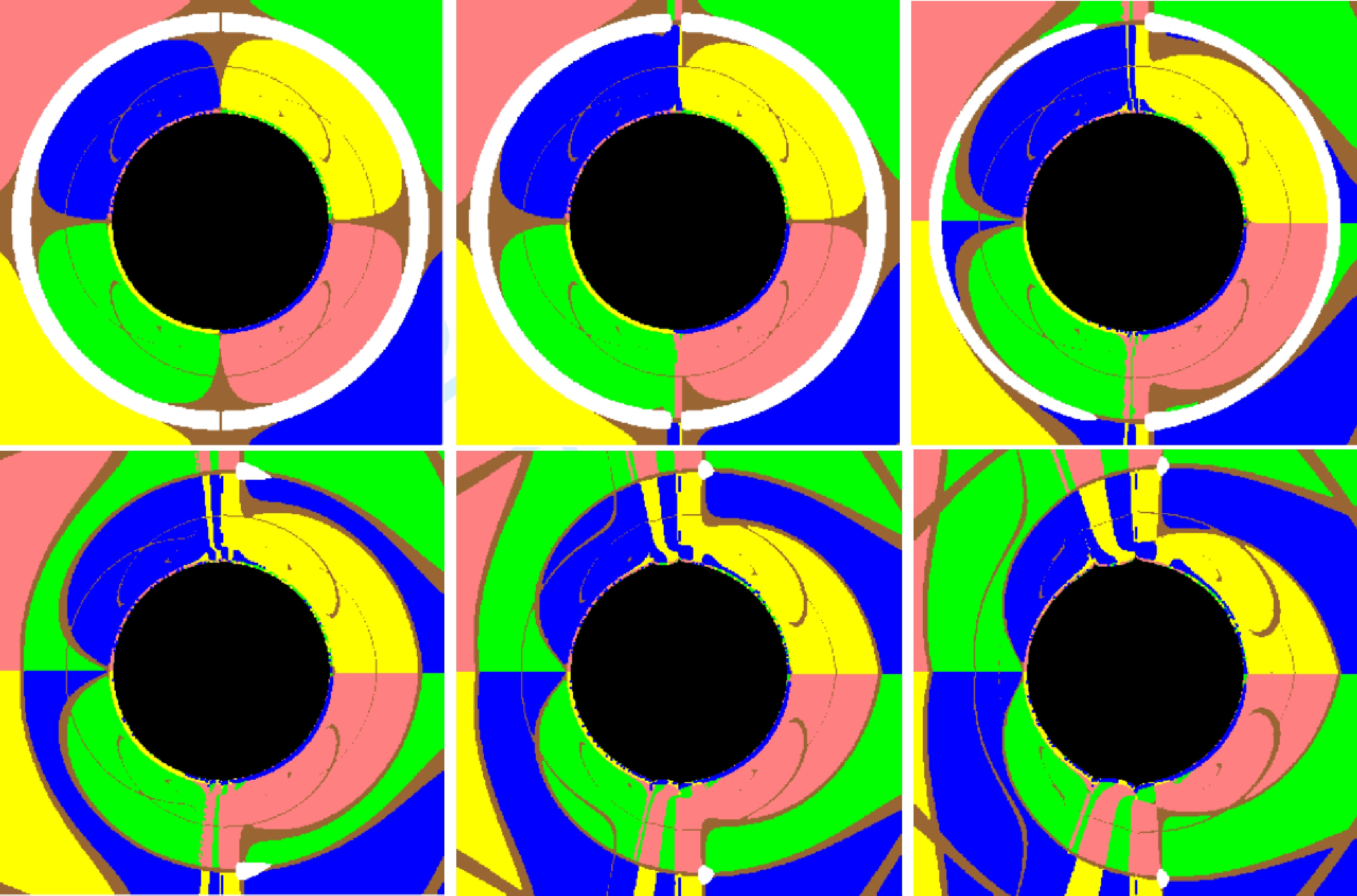
Figure 2. (color online) Black hole images obtained for different spin parameters a. From left to right and then from top to bottom, the values of the spin parameters are 0, 0.01, 0.05, 0.1, 0.2, and 0.3, respectively. The four colors (pink, yellow, blue, and green) correspond to those of the four painted quadrants of the celestial sphere shown in Fig. 1. Brown is associated with the evenly spaced grid lines, and the white Einstein ring is formed by the white dot on the celestial sphere. The dark area mostly located at the center of the image corresponds to the shadow of the black hole.
It is well-known that the spin of the black hole causes a frame-dragging effect. As the spin increases, the frame-dragging effect becomes more apparent. This can be seen by observing how the deformation of the grid lines (brown) becomes more significant with increasing spin. As the direction of the spin is pointing upward, the resulting black hole images and shadows are symmetric about the equator. In contrast, the shape of the black hole shadow is significantly affected by the spin. These results are consistent with those obtained for Kerr black holes.
-
In Fig. 3, we investigate the impact of the black hole charge on its image. The calculations are carried out by taking
$ a=0.05 $ ,$ M=2 $ , Λ= –1, and$ \beta=1 $ , while varying the charge q. For a given value of spin, the frame-dragging effect is apparent. However, the degree of deformation stays mostly the same as the charge of the black hole increases. Moreover, as the charge q gradually increases, the size of the shadow decreases. This is not evident in Fig. 3. In particular, the shadow is surrounded by a complete ring, which decreases with the size of the image, the shape of which largely remains unchanged. This can be understood in terms of Eq. (10), which indicates that the size of the horizon decreases with increasing charge. Although they are two distinct quantities, it is intuitively understood that the size of the shadow is closely associated with that of the horizon.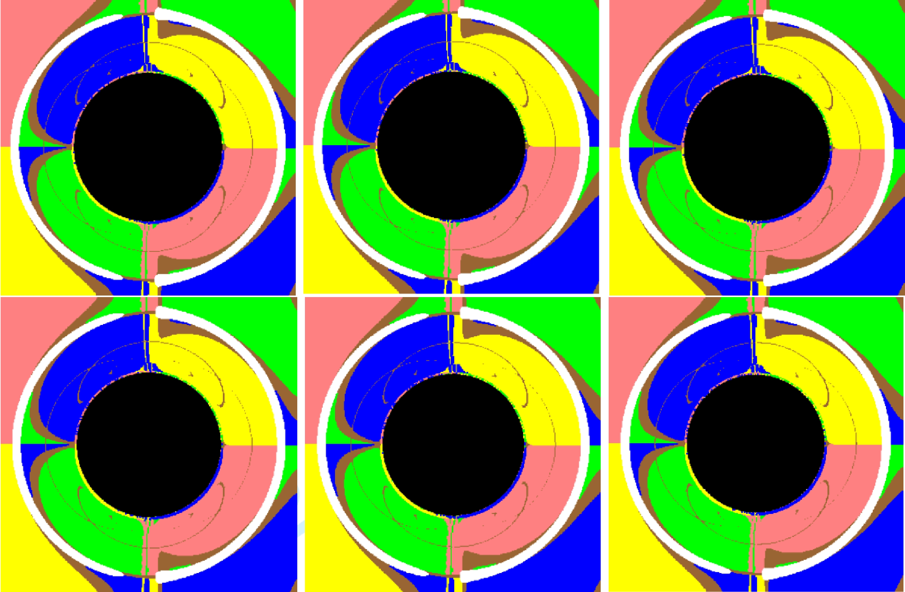
Figure 3. (color online) Black hole images obtained for different charges q. From left to right and then from top to bottom, the values of the charges are 0.4, 0.6, 0.8, 1, 1.2, and 1.4, respectively. The convention of the colors is the same as that in Fig. 2.
-
In Fig. 4, we present the resulting black hole image and shadow for different β values. Here, the calculations are carried out by taking
$ a=0.05 $ ,$ M=2 $ ,$ \Lambda=-1 $ , and$ q=0.01 $ . By varying the nonlinear coupling, one observes some intriguing phenomena. For small values of the coupling, the impact on the frame-dragging is apparent; moreover, it significantly affects the size of the black hole shadow. When the value of the nonlinear coupling parameter is from approximately 0.001 to 0.01, the variation in the black hole shadow is evident. However, as the coupling increases further, both the frame-dragging and the size of the shadow do not significantly change as they converge to given values. In other words, when the value of the nonlinear coupling parameter exceeds approximately 0.01, the change in the black hole shadow is not evident.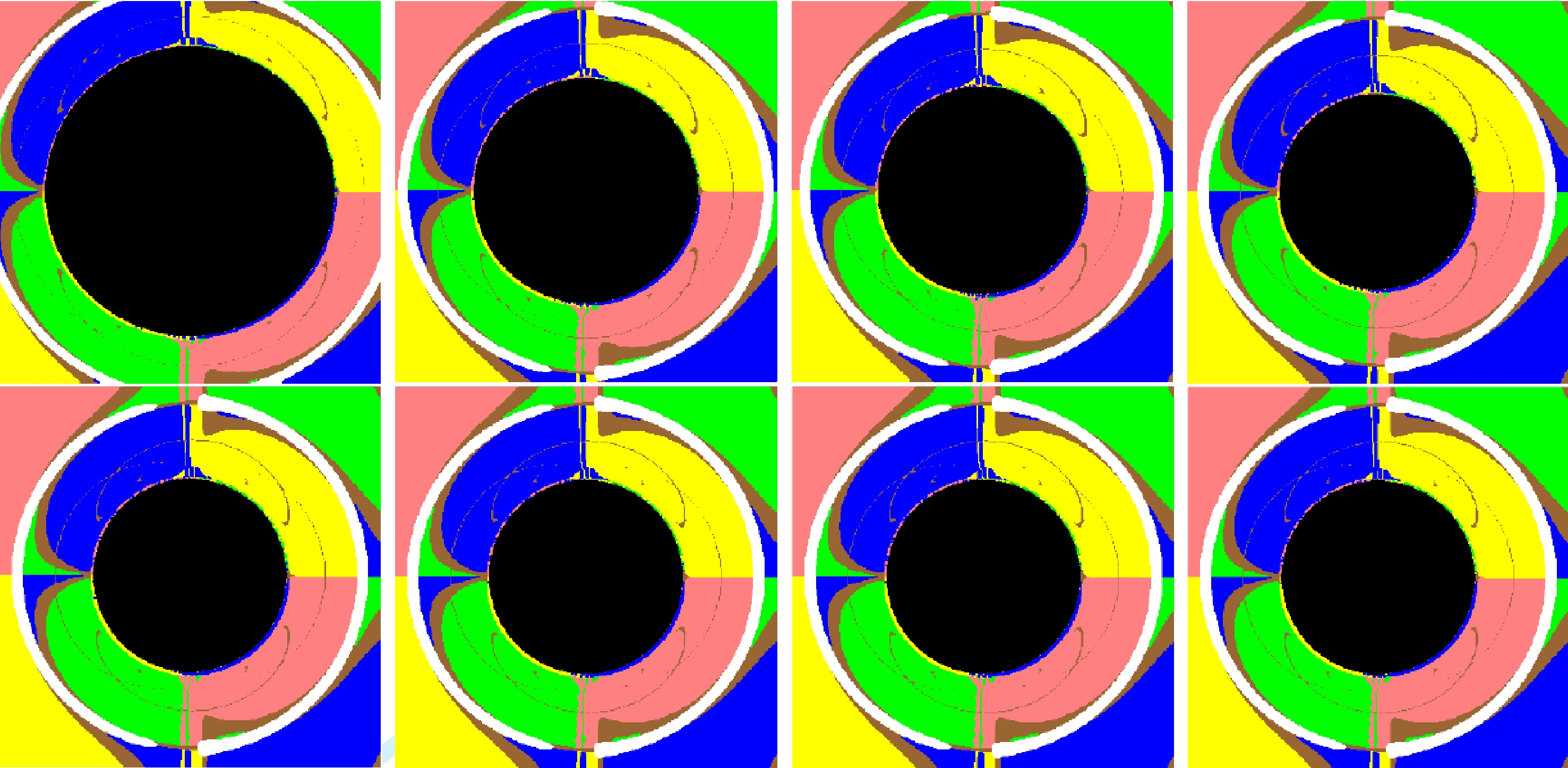
Figure 4. (color online) Black hole images obtained for different nonlinear coupling constants β. From left to right and then from top to bottom, the values of the couplings are 0.001, 0.002, 0.003, 0.01, 0.1, 1, 10, and 100, respectively. The convention of the colors is the same as that in Fig. 2.
Here, in order to analyze the shape characteristics of the black hole shadow in detail, we introduce the black hole shadow radius
$ R_s $ [39].$ R_s $ is the radius of the reference circle defined as passing through three points,$ B(b_1,b_2) $ as the top point,$ C(c_1,c_2) $ as the bottom point, and$ D(d_1,d_2) $ as the right point, by the following expression:$ R_s=\frac{({b_1}-{d_1})^2+{b_2}^2}{2|{b_1}-{d_1}|}. $

(18) In Fig. 5, we show the shadow radius
$ R_s $ as a function of the nonlinear coupling parameter β. The shadow radius$ R_s $ is shown to be sensitive to the nonlinear coupling parameter β, as it decreases with increasing β. This is consistent with changes in the black hole shadow map.
Figure 5. Obtained shadow radius
$ R_s $ as a function of the nonlinear coupling parameter β.Therefore, the above observation breaks the intuitive but rather vague understanding that the size of the shadow is related to that of the horizon. As the nonlinear coupling parameter tends to infinity, the black hole in question approaches the limit of a Kerr-Newman one. This interesting result might lead to observational implications associated with NLED in an astrophysical context.
-
In this section, we consider another feasible option, the exponential form of NLED given in [24]:
$ L(F)=\beta^2\left(\exp\left(-\frac{F}{\beta^2}\right)-1\right) . $

(19) Similarly, the one-form electromagnetic potential reads
$ \begin{array}{*{20}{l}} A=h(r)[{\rm d}t+a\cos\theta {\rm d}\phi] , \end{array} $

(20) where
$ h'(r)=\frac{q}{r^2}\exp\left(\frac{-L_W}{2}\right) , $

(21) where
$ L_W=\mathrm{Lambert}W(4q^2/\beta^2r^4) $ , and$ \mathrm{Lambert}\;W(x) \exp[\mathrm{Lambert}W(x)]=x $ .In this case, the solution of the slowly rotating charged black hole becomes
$ G(r)=1-\frac{2M}{r}-\frac{\Lambda r^2}{3}-\frac{\beta^2r^2}{6}+\frac{\beta q}{r}\left(\int{\frac{{\rm d}r}{\sqrt{L_W}}-\int\sqrt{L_W}{\rm d}r}\right) . $

(22) By employing a similar strategy, one finds the following effective metric:
$ \begin{array}{*{20}{l}} {\rm d}s^2= g_{tt}{\rm d}t^2+g_{rr}{\rm d}r^2+g_{\theta\theta}{\rm d}{\theta}^2+g_{\phi\phi}{\rm d}{\phi}^2+2g_{t\phi}{\rm d}t{\rm d}{\phi}, \end{array} $

where
$ \begin{aligned}[b] g_{tt}=&-\frac{{\rm e}^{-\frac{2q^2}{r^4\beta^2}}r^2\beta^2(-6q^2+r(6M-3r+\Lambda r^3))}{3(4q^2+r^4\beta^2)},\\ g_{rr}=&\frac{3{\rm e}^{-\frac{2q^2}{r^4\beta^2}}r^6\beta^2}{(4q^2+r^4\beta^2)(-6q^2+r(6M-3r+\Lambda r^3))},\\ g_{\theta\theta}=&-{\rm e}^{-\frac{2q^2}{r^4\beta^2}}r^2,\\ g_{\phi\phi}=&-{\rm e}^{-\frac{2q^2}{r^4\beta^2}}r^2\sin^2{\theta},\\ g_{t\phi}=&-\frac{a{\rm e}^{-\frac{2q^2}{r^4\beta^2}}r^2\beta^2(-6q^2+r(6M-3r+\Lambda r^3))\cos{\theta}}{3(4q^2+r^4\beta^2)}, \end{aligned} $

(23) wher M and q correspond to the mass and charge of the black hole, respectively. Again, these quantities only involve second-order terms in q.
The horizons are given by
$ (g_{rr})^{-1}=0 $ , which gives$ \begin{array}{*{20}{l}} -6q^2+r(6M-3r+\Lambda r^3)=0. \end{array} $

(24) The black hole image and shadow can be evaluated using a similar setup to that described before. We elaborate on the dependence of the size and shape of the shadow on various metric parameters. Again, our discussions are divided into three subsections.
-
In Fig. 6, one explores the black hole image and its dependence on the black hole spin. The calculations are carried out by varying the spin parameter a, while taking
$ M=2 $ ,$ q=1 $ , Λ= –1, and$ \beta=1 $ . Similar to that in the logarithmic NLED case, the resulting black hole image is significantly affected by the spin, owing to the frame-dragging effect. For a static black hole with$ a=0 $ , the Einstein ring is visualized chiefly as a circle. As in the logarithmic model, the obtained results can be understood mainly in analogy to the Kerr black hole.
Figure 6. (color online) Black hole images obtained for different spin parameters a. From left to right and then from top to bottom, the values of the spin are 0, 0.01, 0.05, 0.1, 0.2, and 0.3, respectively. The convention of the colors is the same as that in Fig. 2.
-
In Fig. 7, one explores the impact of the charge on the resultant black hole image and shadow. The calculations are carried out by varying the value of q, while taking
$ a=0.05 $ ,$ M=2 $ , Λ= –1, and$ \beta=1 $ . We assume a non-vanishing$ a=0.05 $ , so the frame-dragging effect is apparent. As the charge increases, the size of the shadow decreases, but the change is not evident. This can be understood in terms of the size of the horizon given by Eq. (24). Regarding the image of the background celestial sphere, the main feature, which is governed by the frame-dragging, largely remains unchanged. This result is similar to that in the case of the logarithmic NLED model.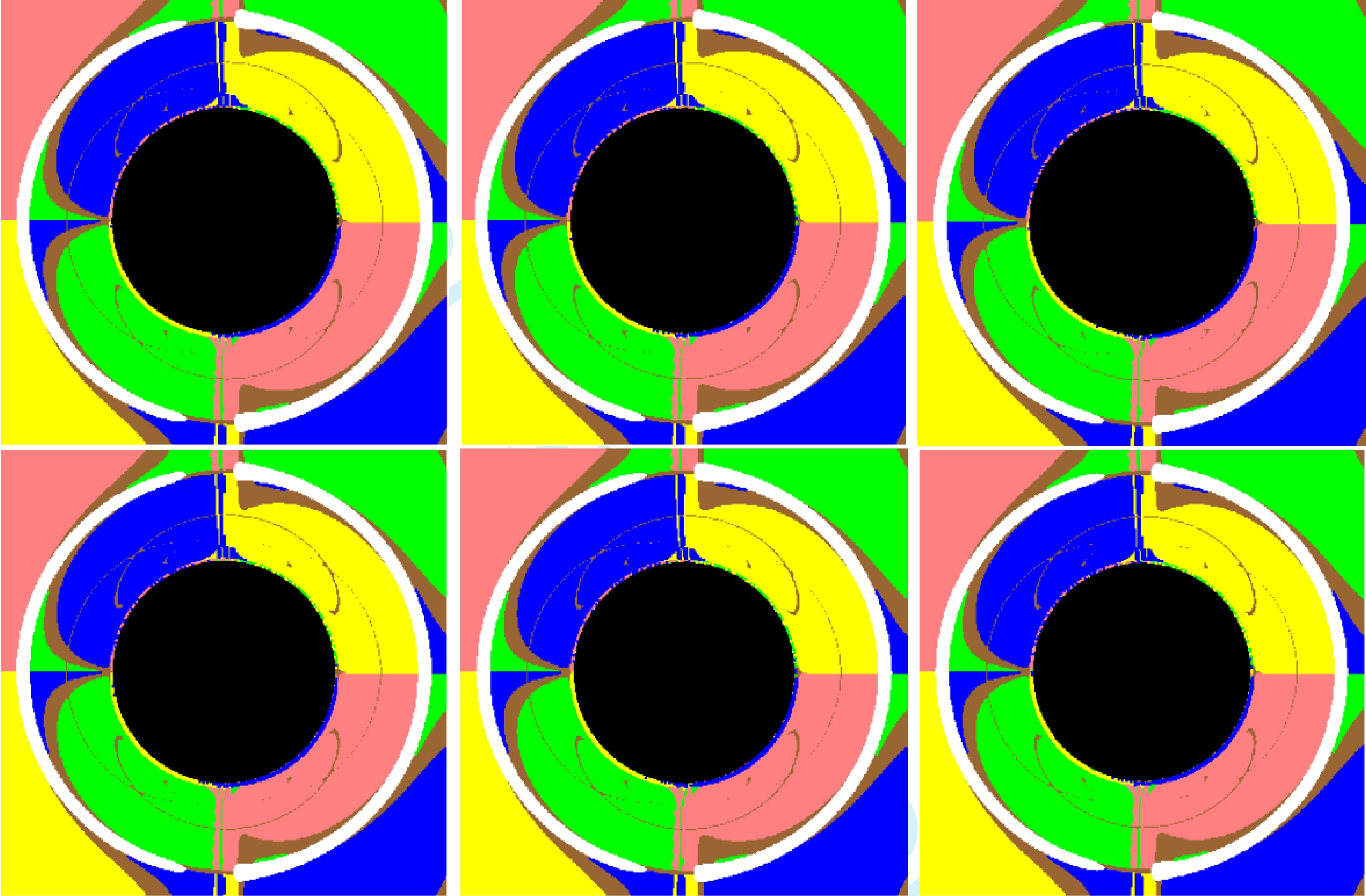
Figure 7. (color online) Black hole images obtained for different charges q. From left to right and then from top to bottom, the values of the charges are 0.1, 0.3, 0.5, 0.7, 0.9, and 1.1, respectively. The convention of the colors is the same as that in Fig. 2.
-
Last but not least, in Fig. 8, we investigate the role of the nonlinear coupling β. Here, the calculations are perfomed using the metric parameters
$ a=0.05 $ ,$ M=2 $ ,$ \Lambda=-1 $ , and$ q=0.01 $ . Some interesting features are observed in the exponential NLED model by gradually increasing the coupling constant. Similar to those in the logarithmic case, the size of the shadow and the details of the image are first sensitive to the coupling and then converge to given forms. Specifically, the size of the black hole shadow decreases with increasing coupling. Its value drops quickly at small β;then, it saturates and approaches a limit. The black hole image demonstrates a more sophisticated pattern that evolves as β decreases. However, it also converges to a well-defined pattern when the coupling becomes sufficiently large. In other words, when the value of the nonlinear coupling parameter is approximately 0.002–0.01, the change in the black hole shadow is very evident, and when it exceeds approximately 0.01, the black hole shadow size hardly changes. Similarly, we plot the radius of the black hole shadow against the nonlinear coupling parameter β. In Fig. 9, we find that the shadow radius of the black hole decreases with an increase in the nonlinear coupling parameter β, which is consistent with the change in the shadow image. 
Figure 8. (color online) Black hole images obtained for different nonlinear coupling constants β. From left to right and then from top to bottom, the values of the nonlinear coupling are 0.002, 0.003, 0.005, 0.01, 0.1, 1, 10, and 100, respectively. The convention of the colors is the same as that inFig. 2.
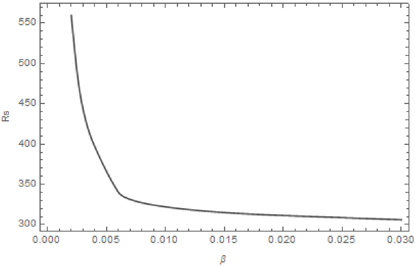
Figure 9. Obtained shadow radius
$ R_s $ as a function of the nonlinear coupling parameter β.Again, we point out that, since the horizon is (mostly) independent of β, the above results cannot be straightforwardly explained in analogy to the results regarding their static/stationary counterparts with linear electrodynamics.
-
In this study, we analyzed the propagation of photons and the resultant black hole images in the medium of NLED. They do not propagate along the null geodesics of the background geometry but of an effective one; this leads to non-trivial implications for the black hole images and shadows. For the present study, we mainly focused on slowly rotating black holes using two different versions of NLED implementations, namely, the logarithmic and exponential models. We evaluated the effective metric and, subsequently, the black hole images and shadows using backward ray-tracing calculations. Moreover, we investigated the impacts of metric parameters on the black hole image. In particular, the nonlinear coupling has been shown to play an essential role in the resulting optical features.
Although some details are distinct, the main features are consistent for both NLED models. The black hole spin a is found to affect the deformation of the black hole image sensitively, but it does not significantly change the size and shape of the shadow. The former can be understood in terms of the frame-dragging effect. The latter, in contrast, can be attributed to the dependence of horizon radius on the spin of the black hole. In particular, due to slow rotation, the spin appears in the models as a higher-order effect. As a result, Eqs. (10) and (24) do not explicitly depend on the spin parameter a, consistent with our arguments. For the charge q, it only changes the size of the black hole shadow through its impact on the black hole horizon. As the charge increases, the change in the shadow of the black hole is not evident. For nonlinear coupling, it is found to have a sizable effect on the black hole image. It plays a sensitive role in the limit of small coupling. However, as the coupling becomes more significant, the image deformation and the shadow size converge into a well-defined form. According to Eqs. (2) and (19), both theories converge to linear electrodynamics at the limit
$ \beta \to \infty $ . Indeed, Figs. 4 and 8, as well as Figs. 5 and 9, indicate that the corresponding black shadows also converge to a limit. Moreover, the deviations owing to the NLED are manifestly significant. As a result, one may argue that once the observation is feasible, such a feature cannot be straightforwardly explained in terms of the counterparts with linear electrodynamics and can potentially lead to astrophysical implications.
Effect of nonlinear electrodynamics on shadows of slowly rotating black holes
- Received Date: 2022-08-29
- Available Online: 2023-02-15
Abstract: In this study, we investigate the effect of nonlinear electrodynamics on the shadows of charged, slowly rotating black holes with the presence of a cosmological constant. Rather than the null geodesic of the background black hole spacetime, the trajectory of a photon, as a perturbation of the nonlinear electrodynamic field, is governed by an effective metric. The latter can be derived by analyzing the propagation of a discontinuity of the electromagnetic waveform. Subsequently, the image of the black hole and its shadow can be evaluated using the backward ray-tracing technique. We explore the properties of the resultant black hole shadows of two different scenarios of nonlinear electrodynamics, namely, the logarithmic and exponential forms. In particular, the effects of nonlinear electrodynamics on the optical image are investigated, as well as the image's dependence on other metric parameters, such as the black hole spin and charge. The resulting black hole image and shadow display rich features that potentially lead to observational implications.


 DownLoad: