


 Abstract
 HTML
HTML Reference
 Related
 PDF
PDF


-
In 2015, the LHCb collaboration observed
$ P_c(4380) $ and$ P_c(4450) $ in the$ J/\psi p $ invariant mass distribution with the favored spin-parity$ J^P={\dfrac{3}{2}}^- $ and$ {\dfrac{5}{2}}^+ $ (rather than the reversed parity$ {\dfrac{3}{2}}^+ $ and$ {\dfrac{5}{2}}^- $ ), respectively, in$ \Lambda_b^0\to J/\psi K^- p $ decays [1]. If these are really resonant states (not re-scattering, threshold, or cusp effects), they must have a minimal valence quark content of$ uudc\bar{c} $ and are excellent pentaquark candidates. In 2019, the LHCb collaboration confirmed the structure$ P_c(4450) $ , which is resolved with two narrow overlapping peaks,$ P_c(4440) $ and$ P_c(4457) $ , with a statistical significance of$ 5.4\,\sigma $ . In addition, they observed a narrow structure,$ P_c(4312) $ , in the$ J/\psi p $ invariant mass distribution, with a statistical significance of$ 7.3\,\sigma $ , in a considerably larger data sample.$ P_c(4312) $ is also an excellent pentaquark candidate with a minimal valence quark content of$ uudc\bar{c} $ [2].In 2020, the LHCb collaboration reported evidence of a new structure,
$ P_{cs}(4459) $ , in the$ J/\psi \Lambda $ invariant mass distribution, with a significance of$ 3.1\sigma $ in$ \Xi_b^- \to J/\psi K^- \Lambda $ decays [3]. If$ P_{cs}(4459) $ is confirmed to be a real resonance, it will be an excellent pentaquark candidate with a minimal valence quark content of$ udsc\bar{c} $ . In fact,$ P_{cs}(4459) $ may also be due to two resonances, as in the case of$ P_c(4450) $ .In 2021, the LHCb collaboration observed evidence of a new structure,
$ P_c(4337) $ , in the$ J/\psi p $ and$ J/\psi \bar{p} $ systems in$ B_s^0 \to J/\psi p \bar{p} $ decays, with a significance in the range$ 3.1-3.7\sigma $ , depending on the assigned$ J^P $ hypothesis [4]. The existence of$ P_c(4337) $ still requires confirmation, and its spin-parity still requires measurement.Recently, the LHCb collaboration observed evidence of a new structure,
$ P_{cs}(4338) $ , in the$ J/\psi \Lambda $ mass distribution in$ B^- \to J/\psi \Lambda \bar{p} $ decays [5]. The measured Breit-Wigner mass and width are$ 4338.2\pm0.7\pm0.4\,\rm{MeV} $ and$ 7.0\pm1.2\pm1.3\,\rm{MeV} $ , respectively, and the favored spin-parity is$ J^P={\dfrac{1}{2}}^- $ .$ P_{cs}(4338) $ and$ P_{cs}(4459) $ are observed in the$ J/\psi \Lambda $ invariant mass distribution and have the isospin$ I=0 $ . Because strong decays conserve the isospin, the observation of their isospin cousins are of crucial importance.The
$ P_c(4312) $ ,$ P_c(4380) $ ,$ P_c(4440) $ ,$ P_c(4457) $ ,$ P_{cs}(4459) $ , and$ P_{cs}(4338) $ lie slightly below or above the thresholds of the charmed meson-baryon pairs$ \bar{D}\Sigma_c $ ,$ \bar{D}\Sigma_c^* $ ,$ \bar{D}^*\Sigma_c $ ,$ \bar{D}^*\Sigma_c $ ,$ \bar{D}\Xi_c^\prime $ ($ \bar{D}\Xi_c^* $ ,$ \bar{D}^*\Xi_c $ ,$ \bar{D}^*\Xi_c^\prime $ ), and$ \bar{D}\Xi_c $ , respectively. Just as we expect,$ P_c(4312) $ ,$ P_c(4380) $ ,$ P_c(4440) $ ,$ P_c(4457) $ ,$ P_{cs}(4459) $ , and$ P_{cs}(4338) $ have been tentatively assigned as charmed meson-baryon molecular states according to several phenomenological analyses [6−12]. Because it is difficult to identify$ P_c(4337) $ as a molecular state without resorting to the help of large coupled-channel effects owing to a lack of nearby meson-baryon thresholds, it is more natural to identify$ P_c(4337) $ as an$ A-A-\bar{c} $ -type hidden-charm pentaquark state with the spin-parity$ J^P={\dfrac{1}{2}}^- $ , where A denotes axial vector diquark states [13].In fact, we can reproduce the masses of
$ P_c(4312) $ ,$ P_c(4337) $ ,$ P_c(4380) $ ,$ P_c(4440) $ ,$ P_c(4457) $ , and$ P_{cs}(4459) $ in the picture of diquark-diquark-antiquark type (or diquark-triquark type) pentaquark states via the theoretical method of QCD sum rules [13, 14].In Ref. [15], we adopt the hadronic dressing mechanism to compromise the pentaquark and molecule interpretations, which are two different schemes that can both give satisfactory experimental masses. The hadronic dressing mechanism was introduced previously to interpret the exotic hierarchy of the masses of scalar mesons below
$ 1 \,\rm{GeV} $ [16−18], and we expect that the same mechanism exists here. Pentaquark states may have a diquark-diquark-antiquark type intrinsic pentaquark kernel,$ qqqc\bar{c} $ , with the typical size of conventional$ qqq $ baryons (approximately$0.5 - 0.7 \;\rm{fm}$ ). The strong couplings of the intrinsic kernels$ qqqc\bar{c} $ to nearby charmed meson-baryon pairs result in molecule components, and the pentaquark states may spend a large time as molecular states; thus, they may display properties of molecules.According to our previous calculations in the framework of QCD sum rules, the lowest diquark-diquark-antiquark type hidden-charm pentaquark state without strange has a mass of approximately
$ 4.31\,\rm{GeV} $ . It is difficult to assign$ P_{cs}(4338) $ as a diquark-diquark-antiquark type pentaquark state with strange, or there is a contradiction in identifying$ P_c(4312) $ and$ P_{cs}(4338) $ in the same picture as pentaquark states. The lowest diquark-diquark-antiquark type hidden-charm pentaquark state with strange has a mass of approximately$ 4.45\,\rm{GeV} $ according to direct calculations in the framework of QCD sum rules and a qualitative analysis based on$S U(3)$ mass-breaking effects [13, 14], which is considerably larger than the mass of$ P_{cs}(4338) $ .In QCD sum rules, we usually choose local currents to interpolate tetraquark or pentaquark molecular states that have two color-neutral clusters [19−25]. It is not necessary for color-neutral clusters to be physical mesons and baryons, they just have the same quantum numbers as physical mesons and baryons. The local currents require that the molecular states have average spatial sizes,
$ \sqrt{\langle r^2\rangle} $ , of the same magnitudes as conventional mesons and baryons, and they must also be compact objects, similar to diquark-antidiquark type tetraquark states or diquark-diquark-antiquark type pentaquark states. It is not necessary for these molecular states to be loosely bound; as conventional mesons and baryons are compact objects, in the local limit, conventional mesons and baryons lose themselves and merge into color-singlet-color-singlet type tetraquark or pentaquark states [26].In this study, we extend our previous studies on pentaquark molecular states to investigate the
$ \bar{D}\Xi_c $ ,$ \bar{D}\Lambda_c $ ,$ \bar{D}_s\Xi_c $ ,$ \bar{D}_s\Lambda_c $ ,$ \bar{D}^*\Xi_c $ ,$ \bar{D}^*\Lambda_c $ ,$ \bar{D}^*_s\Xi_c $ , and$ \bar{D}^*_s\Lambda_c $ molecular states with distinguished isospins in the framework of QCD sum rules [24, 27−29]. We perform operator product expansion consistently up to the vacuum condensates of dimension$ 13 $ , as in previous studies, and determine the best energy scales of the spectral densities using a modified energy-scale formula by considering light-flavor$S U(3)$ mass-breaking effects. Moreover, we attempt to obtain the lowest color-singlet-color-singlet type pentaquark states because one of the color-neutral clusters has the same quantum numbers as the lowest charmed baryons in the flavor anti-triplet and make possible assignments of$ P_{cs}(4338) $ and$ P_{cs}(4459) $ .The paper is arranged as follows. We acquire QCD sum rules for pentaquark molecular states in Sec. II. In Sec. III, we present the numerical results and discussions. Finally, Sec. IV is reserved for our conclusion.
-
First, let us write down the two-point correlation functions
$ \Pi(p) $ and$ \Pi_{\mu\nu}(p) $ ,$ \begin{aligned}[b] \Pi(p)=&{\rm i}\int {\rm d}^4x {\rm e}^{{\rm i}p \cdot x} \langle0|T\left\{J(x)\bar{J}(0)\right\}|0\rangle \, ,\\ \Pi_{\mu\nu}(p)=&{\rm i}\int {\rm d}^4x {\rm e}^{{\rm i}p \cdot x} \langle0|T\left\{J_{\mu}(x)\bar{J}_{\nu}(0)\right\}|0\rangle \, , \end{aligned} $

(1) where the interpolating currents
$ \begin{aligned}[b] J(x)=&J_{(0,0)}^{\bar{D}\Xi_c}(x)\, , \, J_{(1,0)}^{\bar{D}\Xi_c}(x)\, , \, J_{(\frac{1}{2},\frac{1}{2})}^{\bar{D}\Lambda_c}(x)\, , \, J_{(\frac{1}{2},\frac{1}{2})}^{\bar{D}_s\Xi_c}(x)\, , \, J_{(0,0)}^{\bar{D}_s\Lambda_c}(x)\, , \\ J_\mu(x)=&J_{(0,0)}^{\bar{D}^*\Xi_c}(x)\, , \,J_{(1,0)}^{\bar{D}^*\Xi_c}(x)\, , \,J_{(\frac{1}{2},\frac{1}{2})}^{\bar{D}^*\Lambda_c}(x)\, , \,J_{(\frac{1}{2},\frac{1}{2})}^{\bar{D}_s^*\Xi_c}(x)\, , \, J_{(0,0)}^{\bar{D}_s^*\Lambda_c}(x)\, , \end{aligned} $

(2) $ \begin{aligned}[b] J_{(0,0)}^{\bar{D}\Xi_c}(x)=&\frac{1}{\sqrt{2}}J_{\bar{D}^0}(x)J_{\Xi_c^{0}}(x)-\frac{1}{\sqrt{2}}J_{\bar{D}^-}(x)J_{\Xi_c^+}(x) \, , \\ J_{(1,0)}^{\bar{D}\Xi_c}(x)=&\frac{1}{\sqrt{2}}J_{\bar{D}^0}(x)J_{\Xi_c^{0}}(x)+\frac{1}{\sqrt{2}}J_{\bar{D}^-}(x)J_{\Xi_c^+}(x) \, , \\ J_{(\frac{1}{2},\frac{1}{2})}^{\bar{D}\Lambda_c}(x)=&J_{\bar{D}^0}(x)J_{\Lambda_c^+}(x) \, , \\ J_{(\frac{1}{2},\frac{1}{2})}^{\bar{D}_s\Xi_c}(x)=&J_{\bar{D}^-_s}(x)J_{\Xi_c^+}(x) \, , \\ J_{(0,0)}^{\bar{D}_s\Lambda_c}(x)=&J_{\bar{D}^-_s}(x)J_{\Lambda_c^+}(x) \, , \end{aligned} $

(3) $ \begin{aligned}[b] J_{(0,0)}^{\bar{D}^*\Xi_c}(x)=&\frac{1}{\sqrt{2}}J_{\bar{D}^{*0}}(x)J_{\Xi_c^{0}}(x)-\frac{1}{\sqrt{2}}J_{\bar{D}^{*-}}(x)J_{\Xi_c^+}(x) \, , \\ J_{(1,0)}^{\bar{D}^*\Xi_c}(x)=&\frac{1}{\sqrt{2}}J_{\bar{D}^{*0}}(x)J_{\Xi_c^{0}}(x)+\frac{1}{\sqrt{2}}J_{\bar{D}^{*-}}(x)J_{\Xi_c^+}(x) \, , \\ J_{(\frac{1}{2},\frac{1}{2})}^{\bar{D}^*\Lambda_c}(x)=&J_{\bar{D}^{*0}}(x)J_{\Lambda_c^+}(x) \, , \\ J_{(\frac{1}{2},\frac{1}{2})}^{\bar{D}^*_s\Xi_c}(x)=&J_{\bar{D}^{*-}_s}(x)J_{\Xi_c^+}(x) \, , \\ J_{(0,0)}^{\bar{D}^*_s\Lambda_c}(x)=&J_{\bar{D}^{*-}_s}(x)J_{\Lambda_c^+}(x) \, , \end{aligned} $

(4) and
$ \begin{aligned}[b] J_{\bar{D}^0}(x)=&\bar{c}(x){\rm i}\gamma_5u(x)\, , \\ J_{\bar{D}^-}(x)=&\bar{c}(x){\rm i}\gamma_5d(x)\, , \\ J_{\bar{D}_s^-}(x)=&\bar{c}(x){\rm i}\gamma_5s(x)\, , \\ J_{\bar{D}^{*0}}(x)=&\bar{c}(x)\gamma_\mu u(x)\, , \\ J_{\bar{D}^{*-}}(x)=&\bar{c}(x)\gamma_\mu d(x)\, , \\ J_{\bar{D}_s^{*-}}(x)=&\bar{c}(x)\gamma_\mu s(x)\, , \\ J_{\Xi_c^{ 0}}(x)=&\varepsilon^{ijk}d^{T}_i(x)C\gamma_{5}s_j(x) c_k(x)\, ,\\ J_{\Xi_c^{ +}}(x)=&\varepsilon^{ijk}u^{T}_i(x)C\gamma_{5}s_j(x) c_k(x)\, ,\\ J_{\Lambda_c^{ +}}(x)=&\varepsilon^{ijk}u^{T}_i(x)C\gamma_{5}d_j(x) c_k(x)\, , \end{aligned} $

(5) where the super(sub)scripts
$ i, j, k $ are color indices, and C represents the charge conjugation matrix.$ J_{\bar{D}^0}(x) $ ,$ J_{\bar{D}^-}(x) $ ,$ J_{\bar{D}_s^-}(x) $ ,$ J_{\bar{D}^{*0}}(x) $ ,$ J_{\bar{D}^{*-}}(x) $ ,$ J_{\bar{D}_s^{*-}}(x) $ ,$ J_{\Xi_c^{ 0}}(x) $ ,$ J_{\Xi_c^{ +}}(x) $ , and$ J_{\Lambda_c^{ +}}(x) $ are commonly used meson and baryon currents, and the subscripts$ (1,0) $ ,$ (0,0) $ , and$ (\dfrac{1}{2},\dfrac{1}{2}) $ represent the isospins$ (I,I_3) $ .According to quark-hadron duality, the currents
$ J(0) $ couple potentially to hidden-charm molecular states with the spin-parity$ J^P={\dfrac{1}{2}}^\pm $ , whereas the currents$ J_\mu(0) $ couple potentially to hidden-charm molecular states with the spin-parity$ J^P={\dfrac{1}{2}}^\pm $ and$ {\dfrac{3}{2}}^\pm $ ,$ \begin{aligned}[b] \langle 0| J (0)|P^-_{\frac{1}{2}}(p)\rangle =&\lambda^-_{\frac{1}{2}} U^-(p,s) \, , \\ \langle 0| J (0)|P^+_{\frac{1}{2}}(p)\rangle =&\lambda^+_{\frac{1}{2}}{\rm i}\gamma_5 U^+(p,s) \, , \end{aligned} $

(6) $ \begin{aligned}[b] \langle 0| J_\mu (0)|P^-_{\frac{1}{2}}(p)\rangle =&f_{\frac{1}{2}}^- p_\mu {\rm i}\gamma_5 U^-(p,s) \, , \\ \langle 0| J_\mu (0)|P^+_{\frac{1}{2}}(p)\rangle =&f_{\frac{1}{2}}^+p_\mu U^+(p,s) \, , \\ \langle 0| J_\mu (0)|P^-_{\frac{3}{2}}(p)\rangle =&\lambda_{\frac{3}{2}}^- U^-_\mu(p,s) \, , \\ \langle 0| J_\mu (0)|P^+_{\frac{3}{2}}(p)\rangle =&\lambda_{\frac{3}{2}}^+{\rm i}\gamma_5 U_\mu^+(p,s) \, , \end{aligned} $

(7) where
$ \lambda^{\pm}_{\frac{1}{2}} $ ,$ \lambda^{\pm}_{\frac{3}{2}} $ , and$ f^{\pm}_{\frac{1}{2}} $ are current-molecule coupling constants (or pole residues), and$ U^\pm(p,s) $ and$ U_\mu^\pm(p,s) $ are Dirac spinors and Rarita-Schwinger spinors, respectively [13, 24, 30, 31].At the hadron side of the correlation functions
$ \Pi(p) $ and$ \Pi_{\mu\nu}(p) $ , we isolate the ground state contributions from the hidden-charm molecular states with the spin-parity$ J^P={\dfrac{1}{2}}^\pm $ and$ {\dfrac{3}{2}}^\pm $ , respectively, and acquire the hadronic representation [13, 24, 30, 31],$ \begin{aligned}[b] \Pi(p) = & \left(\lambda^-_{\frac{1}{2}}\right)^2 {\not {p}+ M_- \over M_-^{2}-p^{2} } + \left(\lambda^+_{\frac{1}{2}}\right)^2 {\not {p}- M_+ \over M_+^{2}-p^{2} } +\cdots \, ,\\ =&\Pi^1_{\frac{1}{2}}(p^2)\not {p}+\Pi^0_{\frac{1}{2}}(p^2)\, ,\\ \Pi_{\mu\nu}(p) = & \left(\lambda^-_{\frac{3}{2}}\right)^2 {\not {p}+ M_- \over M_-^{2}-p^{2} }(-g_{\mu\nu}) + \left(\lambda^+_{\frac{3}{2}}\right)^2 {\not {p}- M_+ \over M_+^{2}-p^{2} }(-g_{\mu\nu}) +\cdots \, ,\\ =&-\Pi^1_{\frac{3}{2}}(p^2)\not {p}g_{\mu\nu}-\Pi^0_{\frac{3}{2}}(p^2)g_{\mu\nu}+\cdots \, , \end{aligned} $

(8) where we choose the components
$ \Pi^{1/0}_{\frac{1}{2}}(p^2) $ and$ \Pi^{1/0}_{\frac{3}{2}}(p^2) $ to explore the molecular states with the spin-parity$ J^P={\dfrac{1}{2}}^- $ and$ {\dfrac{3}{2}}^- $ , respectively.In the following, we omit the subscripts of the pole residues and correlation functions from the above equations (see Eqs.(6)–(8)) and mark them as
$ \lambda_\pm $ and$ \Pi^{1/0}(s) $ , respectively. A direct method of obtaining the hadronic spectral densities is through the dispersion relation,$ \frac{{\rm Im}\Pi^1(s)}{\pi}=\lambda^{2}_- \delta\left(s-M_-^2\right)+\lambda_+^2 \delta\left(s-M_+^2\right) =\, \rho^1_{H}(s) \, , $

(9) $ \frac{{\rm Im}\Pi^0(s)}{\pi}=M_-\lambda_-^2 \delta\left(s-M_-^2\right)-M_+\lambda_+^2 \delta\left(s-M_+^2\right) =\rho^0_{H}(s) \, , $

(10) where we introduce the index H to represent the hadron side. We then obtain QCD sum rules on the hadron side with the help of the weight functions
$ \sqrt{s}\exp\left(-\dfrac{s}{T^2}\right) $ and$ \exp\left(-\dfrac{s}{T^2}\right) $ ,$ \int_{4m_c^2}^{s_0}{\rm d}s \left[\sqrt{s}\rho^1_{H}(s)+\rho^0_{H}(s)\right]\exp\left( -\frac{s}{T^2}\right) =2M_-\lambda_-^2\exp\left( -\frac{M_-^2}{T^2}\right) \, , $

(11) where
$ s_0 $ represents the continuum threshold parameters, and$ T^2 $ represents the Borel parameters.It is also direct to perform operator product expansion routinely [13, 24, 30, 31]. We contract the u, d, s, and c quark fields in the correlation functions
$ \Pi(p) $ and$ \Pi_{\mu\nu}(p) $ using Wick's theorem and observe that there are three full light-quark propagators ($ U_{ij}(x) $ ,$ D_{ij}(x) $ , and$ S_{ij}(x) $ in the coordinate space) and two full charm-quark propagators ($ C_{ij}(x) $ in the momentum space),$ \begin{aligned}[b] U/D_{ij}(x)=& \frac{{\rm i}\delta_{ij}\not {x}}{ 2\pi^2x^4}-\frac{\delta_{ij}\langle \bar{q}q\rangle}{12} -\frac{\delta_{ij}x^2\langle \bar{q}g_s\sigma Gq\rangle}{192} \\&-\frac{{\rm i}g_sG^{a}_{\alpha\beta}t^a_{ij}(\not {x} \sigma^{\alpha\beta}+\sigma^{\alpha\beta} \not {x})}{32\pi^2x^2} -\frac{\delta_{ij}x^4\langle \bar{q}q \rangle\langle g_s^2 GG\rangle}{27648} \\ & -\frac{1}{8}\langle\bar{q}_j\sigma^{\mu\nu}q_i \rangle \sigma_{\mu\nu}+\cdots \, , \end{aligned} $

(12) $ \begin{aligned}[b] S_{ij}(x)=& \frac{{\rm i}\delta_{ij}\not {x}}{ 2\pi^2x^4} -\frac{\delta_{ij}m_s}{4\pi^2x^2}-\frac{\delta_{ij}\langle \bar{s}s\rangle}{12} +\frac{{\rm i}\delta_{ij}\not {x}m_s \langle\bar{s}s\rangle}{48}\\&-\frac{\delta_{ij}x^2\langle \bar{s}g_s\sigma Gs\rangle}{192}+\frac{{\rm i}\delta_{ij}x^2\not {x} m_s\langle \bar{s}g_s\sigma Gs\rangle }{1152}\\ & -\frac{{\rm i}g_s G^{a}_{\alpha\beta}t^a_{ij}(\not {x} \sigma^{\alpha\beta}+\sigma^{\alpha\beta} \not {x})}{32\pi^2x^2} -\frac{\delta_{ij}x^4\langle \bar{s}s \rangle\langle g_s^2 GG\rangle}{27648}\\&-\frac{1}{8}\langle\bar{s}_j\sigma^{\mu\nu}s_i \rangle \sigma_{\mu\nu} +\cdots \, , \end{aligned} $

(13) $ \begin{aligned}[b] C_{ij}(x)=&\frac{\rm i}{(2\pi)^4}\int {\rm d}^4k {\rm e}^{-{\rm i}k \cdot x} \\&\times\left\{ \frac{\delta_{ij}}{\not {k}-m_c} -\frac{g_sG^n_{\alpha\beta}t^n_{ij}}{4}\frac{\sigma^{\alpha\beta}(\not {k}+m_c)+(\not {k}+m_c) \sigma^{\alpha\beta}}{(k^2-m_c^2)^2}\right.\\ &\left. -\frac{g_s^2 (t^at^b)_{ij} G^a_{\alpha\beta}G^b_{\mu\nu}(f^{\alpha\beta\mu\nu}+f^{\alpha\mu\beta\nu}+f^{\alpha\mu\nu\beta}) }{4(k^2-m_c^2)^5}+\cdots\right\} \, ,\\ f^{\alpha\beta\mu\nu}=&(\not{k}+m_c)\gamma^\alpha(\not {k}+m_c)\gamma^\beta(\not {k}+m_c)\gamma^\mu(\not {k}+m_c)\gamma^\nu(\not {k}+m_c)\, , \end{aligned} $

(14) where
$ t^n=\dfrac{\lambda^n}{2} $ , with$ \lambda^n $ being the Gell-Mann matrix [32–34]. If each charm-quark line emits a gluon and each light-quark line contributes a quark-antiquark pair, we acquire the quark-gluon operator$ g_s^2G_{\alpha\beta}G^{\alpha\beta}\bar{q}q \bar{q}q \bar{q}q $ (with$ q=u $ , d, or s) of dimension 13; therefore, we must deal with condensates up to at least dimension 13 to judge the convergent behavior of operator product expansion because the condensates are vacuum expectations of quark-gluon operators in the QCD vacuum.We retain the possible operators
$ \langle\bar{q}_j\sigma_{\mu\nu}q_i \rangle $ and$ \langle\bar{s}_j\sigma_{\mu\nu}s_i \rangle $ from the Fierz transformations of the quark operators$ \langle q_i \bar{q}_j\rangle $ and$ \langle s_i \bar{s}_j\rangle $ (before Wick's contractions) to absorb the gluons emitted from other quark lines and thus extract the mixed condensates$ \langle\bar{q}g_s\sigma G q\rangle $ and$ \langle\bar{s}g_s\sigma G s\rangle $ , respectively [34]. Then, we sequentially compute all the integrals in the coordinate and momentum spaces to obtain the representations at the quark-gluon level.We count the vacuum condensates using the strong fine structure constant
$ \alpha_s=\dfrac{g_s^2}{4\pi} $ with the orders$ \mathcal{O}( \alpha_s^{k}) $ , where$ k=0 $ ,$ \dfrac{1}{2} $ ,$ 1 $ ,$ \dfrac{3}{2} $ ,$ \cdots $ . In this study, we consistently prefer the truncation$ k\leq 1 $ and deal with the quark-gluon operators of the orders$ \mathcal{O}( \alpha_s^{k}) $ with$ k\leq 1 $ . To be more precise and concrete, we consistently take account of the vacuum condensates$ \langle\bar{q}q\rangle $ ,$ \langle\frac{\alpha_{s}GG}{\pi}\rangle $ ,$ \langle\bar{q}g_{s}\sigma Gq\rangle $ ,$ \langle\bar{q}q\rangle^2 $ ,$ \langle\bar{q}q\rangle \langle\frac{\alpha_{s}GG}{\pi}\rangle $ ,$ \langle\bar{q}q\rangle \langle\bar{q}g_{s}\sigma Gq\rangle $ ,$ \langle\bar{q}q\rangle^3 $ ,$ \langle\bar{q}g_{s}\sigma Gq\rangle^2 $ ,$ \langle\bar{q}q\rangle^2 \langle\frac{\alpha_{s}GG}{\pi}\rangle $ ,$ \langle\bar{q} q\rangle^2\langle\bar{q}g_s\sigma Gq\rangle $ ,$ \langle\bar{q} q\rangle \langle\bar{q}g_s\sigma Gq\rangle^2 $ , and$ \langle \bar{q}q\rangle^3\langle \frac{\alpha_s}{\pi}GG\rangle $ with the assumption of vacuum saturation to assess the convergent behaviors [35], where$ q=u $ , d, or s. In addition, we set the masses of the u and d quarks to be zero and consider the contributions of the order$ \mathcal{O}(m_s) $ consistently for the s quark so as to take account of light-flavor$S U(3)$ mass-breaking effects.Finally, we acquire the QCD spectral densities
$ \rho^1_{\rm QCD}(s) $ and$ \rho^0_{\rm QCD}(s) $ through the dispersion relation (their explicit expressions are available by contacting the corresponding author via email). We then assume (and implement) quark-hadron duality below the continuum thresholds$ s_0 $ and again acquire QCD sum rules with the help of the weight functions$ \sqrt{s}\exp\left(-\dfrac{s}{T^2}\right) $ and$ \exp\left(-\dfrac{s}{T^2}\right) $ :$\begin{aligned}[b] 2M_-\lambda_-^2\exp\left( -\frac{M_-^2}{T^2}\right) =& \int_{4m_c^2}^{s_0}{\rm d}s \left[\sqrt{s}\rho^1_{\rm QCD}(s)+\rho^0_{\rm QCD}(s)\right]\\&\times\exp\left( -\frac{s}{T^2}\right)\, . \end{aligned} $

(15) We differentiate Eq. (15) in regard to
$ \tau=\dfrac{1}{T^2} $ and then delete the pole residues$ \lambda_{-} $ by adopting a fraction to obtain QCD sum rules for the molecule masses,$ M^2_-= \frac{-\dfrac{\rm d}{{\rm d} \tau}\displaystyle\int_{4m_c^2}^{s_0}{\rm d}s \,\left[\sqrt{s}\,\rho^1_{\rm QCD}(s)+\,\rho^0_{\rm QCD}(s)\right]\exp\left(- \tau s\right)}{\displaystyle\int_{4m_c^2}^{s_0}{\rm d}s \left[\sqrt{s}\,\rho_{\rm QCD}^1(s)+\,\rho^0_{\rm QCD}(s)\right]\exp\left( -\tau s\right)}\, . $

(16) -
At the beginning points, we take the conventional (or commonly used) values of the vacuum condensates
$\langle\bar{q}q \rangle = -(0.24\pm 0.01\, \rm{GeV})^3$ ,$\langle\bar{s}s \rangle = (0.8\pm0.1)\langle\bar{q}q \rangle$ ,$\langle\bar{q}g_s\sigma G q \rangle = m_0^2\langle \bar{q}q \rangle$ ,$ \langle\bar{s}g_s\sigma G s \rangle=m_0^2\langle \bar{s}s \rangle $ ,$m_0^2=(0.8 \pm 0.1)\, \rm{GeV}^2$ , and$\langle \frac{\alpha_s GG}{\pi}\rangle = 0.012\pm0.004\,\rm{GeV}^4$ at the energy scale$ \mu=1\, \rm{GeV} $ [32, 36, 37] and take the$\rm \overline{MS} $ masses$m_{c}(m_c)= (1.275\pm 0.025)\,\rm{GeV}$ and$ m_s(\mu=2\,\rm{GeV})=(0.095\pm0.005)\,\rm{GeV} $ from the Particle Data Group [38]. Then, we take account of the energy-scale dependence of all the input parameters [39],$ \begin{aligned}[b] \langle\bar{q}q \rangle(\mu)=&\langle\bar{q}q\rangle({\rm 1 GeV})\left[\frac{\alpha_{s}({\rm 1 GeV})}{\alpha_{s}(\mu)}\right]^{\textstyle\frac{12}{33-2n_f}}\, , \\ \langle\bar{s}s \rangle(\mu)=&\langle\bar{s}s \rangle({\rm 1 GeV})\left[\frac{\alpha_{s}({\rm 1 GeV})}{\alpha_{s}(\mu)}\right]^{\textstyle\frac{12}{33-2n_f}}\, , \\ \langle\bar{q}g_s \sigma Gq \rangle(\mu)=&\langle\bar{q}g_s \sigma Gq \rangle({\rm 1 GeV})\left[\frac{\alpha_{s}({\rm 1 GeV})}{\alpha_{s}(\mu)}\right]^{\textstyle\frac{2}{33-2n_f}}\, ,\\ \langle\bar{s}g_s \sigma Gs \rangle(\mu)=&\langle\bar{s}g_s \sigma Gs \rangle({\rm 1 GeV})\left[\frac{\alpha_{s}({\rm 1 GeV})}{\alpha_{s}(\mu)}\right]^{\textstyle\frac{2}{33-2n_f}}\, ,\\ m_c(\mu)=&m_c(m_c)\left[\frac{\alpha_{s}(\mu)}{\alpha_{s}(m_c)}\right]^{\textstyle\frac{12}{33-2n_f}} \, ,\\ m_s(\mu)=&m_s({\rm 2GeV} )\left[\frac{\alpha_{s}(\mu)}{\alpha_{s}({\rm 2GeV})}\right]^{\textstyle\frac{12}{33-2n_f}}\, ,\\ \alpha_s(\mu)=&\frac{1}{b_0t}\left[1-\frac{b_1}{b_0^2}\frac{\log t}{t} +\frac{b_1^2(\log^2{t}-\log{t}-1)+b_0b_2}{b_0^4t^2}\right]\, , \end{aligned} $

(17) where
$ t=\log \dfrac{\mu^2}{\Lambda^2} $ ,$ b_0=\dfrac{33-2n_f}{12\pi} $ ,$ b_1=\dfrac{153-19n_f}{24\pi^2} $ ,$b_2=\dfrac{2857-\frac{5033}{9}n_f+\frac{325}{27}n_f^2}{128\pi^3}$ , and$ \Lambda=213\,\rm{MeV} $ ,$ 296\,\rm{MeV} $ , and$ 339\,\rm{MeV} $ for the quark flavors$ n_f=5 $ ,$ 4 $ , and$ 3 $ , respectively [38, 39], and evolve them from the energy scales$ \mu=1\,\rm{GeV} $ ,$ m_c $ , and$ 2\,\rm{GeV} $ to a particular uniform energy scale μ in the QCD sum rules for a molecular state to extract the hadron mass.In this study, we explore the lowest hidden-charm molecular states without strange, with strange, and with double strange, and it is better to choose the quark flavor numbers
$ n_f=4 $ and evolve all the input parameters to the particular energy scales μ, which satisfy the modified energy scale formula$ \mu=\sqrt{M^2_{X/Y/Z/P}-(2{\mathbb{M}}_c)^2}-k\,\mathbb{M}_s $ , with the effective c-quark mass$ {\mathbb{M}}_c=1.85\pm0.01\,\rm{GeV} $ and effective s-quark mass$ \mathbb{M}_s=0.2\,\rm{GeV} $ . Here, the subscripts X, Y, Z, and P denote exotic states with hidden-charm, and we take account of light-flavor$S U(3)$ mass-breaking effects by counting the s-quark numbers$ k=0 $ ,$ 1 $ , and$ 2 $ to assess their impact on choosing the energy scales [20, 40].In the hidden-charm (or hidden-bottom) four- and five-quark systems
$ Q\bar{Q}q \bar{q}^\prime $ and$ Q\bar{Q}qq^{\prime}q^{\prime\prime} $ , we explicitly discriminate the heavy and light degrees of freedom and describe them as$ 2{\mathbb{M}}_Q $ and$ \mu+k\,\mathbb{M}_s $ , respectively. We assume that the hadron masses satisfy a Regge-trajectory-like relation, that is,$ M^2_{X/Y/Z/P}=(\mu+k\,\mathbb{M}_s)^2+C\, , $

(18) where the constant
$ C=4{\mathbb{M}}_Q^2 $ , and fit the effective masses$ {\mathbb{M}}_Q $ and$ \mathbb{M}_s $ using the QCD sum rules themselves. Direct and explicit calculations indicate that$ {\mathbb{M}}_Q $ and$ \mathbb{M}_s $ have universal values and work well for all exotic X, Y, Z, and P states. We only use the universal parameters$ {\mathbb{M}}_Q $ and$ \mathbb{M}_s $ to determine the appropriate energy scales μ of the QCD spectral densities in a self-consistent manner. In the QCD spectral densities, we take the$\rm\overline{MS}$ (modified minimal subtraction scheme) quark masses. The modified energy scale formula is a powerful and useful constraint to obey. On the other hand, if we set$ M^2_{X/Y/Z/P}=(\mu+k\,\mathbb{M}_s+2\mathbb{M}_Q)^2\, , $

(19) and take the best energy scales
$ \mu=1.3\,\rm{GeV} $ and$ 2.2\,\rm{GeV} $ for$ Z_c(3900) $ and$ P_c(4312) $ , respectively, as the input parameters [20, 28], we obtain the effective c-quark mass$ {\mathbb{M}}_c=1.30\,\rm{GeV} $ and$ 1.06\,\rm{GeV} $ , respectively, and no uniform/self-consistent parameter can be reached.We search for suitable Borel parameters and continuum threshold parameters to obey the two elementary criteria of QCD sum rules (pole dominance and convergence of operator product expansion play an essential role to warrant reliability) via trial and error. However, it is not easy to achieve such requirements for multiquark states. Because the spectra of exotic states are unclear, we have no robust guide to choose the continuum thresholds, and the two criteria manifest themselves in this aspect. We then acquire the Borel windows and continuum threshold parameters and therefore the optimal energy scales of the QCD spectral densities and pole contributions of the ground states, which are all presented in Table 1.
$ (I,I_3) $ 

$\mu/\rm GeV$ 

$T^2 /\rm{GeV}^2$ 

$\sqrt{s_0}/\rm{GeV}$ 

pole $ \bar{D}\,\Xi_c $ 

$ (0,0) $ 

2.1 $ 3.2-3.8 $ 

$ 5.00\pm0.10 $ 

$40\%-60\%$ 

$ \bar{D}\,\Xi_c $ 

$ (1,0) $ 

2.3 $ 3.1-3.7 $ 

$ 5.09\pm0.10 $ 

$42\%-61\%$ 

$ \bar{D}\,\Lambda_c $ 

$(\dfrac{1}{2},\dfrac{1}{2})$ 

2.5 $ 3.2-3.8 $ 

$ 5.11\pm0.10 $ 

$42\%-60\%$ 

$ \bar{D}_s\,\Xi_c $ 

$ (\dfrac{1}{2},\dfrac{1}{2}) $ 

2.2 $ 3.2-3.8 $ 

$ 5.15\pm0.10 $ 

$41\%-59\%$ 

$ \bar{D}_s\,\Lambda_c $ 

$ (0,0) $ 

2.3 $ 3.2-3.8 $ 

$ 5.13\pm0.10 $ 

$43\%-61\%$ 

$ \bar{D}^*\,\Xi_c $ 

$ (0,0) $ 

2.3 $ 3.2-3.8 $ 

$ 5.10\pm0.10 $ 

$43\%-61\%$ 

$ \bar{D}^*\,\Xi_c $ 

$ (1,0) $ 

2.6 $ 3.3-3.9 $ 

$ 5.27\pm0.10 $ 

$43\%-61\%$ 

$ \bar{D}^*\,\Lambda_c $ 

$ (\dfrac{1}{2},\dfrac{1}{2}) $ 

2.7 $ 3.3-3.9 $ 

$ 5.23\pm0.10 $ 

$41\%-61\%$ 

$ \bar{D}^*_s\,\Xi_c $ 

$ (\dfrac{1}{2},\dfrac{1}{2}) $ 

2.4 $ 3.3-3.9 $ 

$ 5.28\pm0.10 $ 

$42\%-59\%$ 

$ \bar{D}^*_s\,\Lambda_c $ 

$ (0,0) $ 

2.4 $ 3.2-3.8 $ 

$ 5.14\pm0.10 $ 

$42\%-60\%$ 

Table 1. Best energy scales μ, Borel windows
$ T^2 $ , continuum threshold parameters$ s_0 $ , and pole contributions (pole) for hidden-charm pentaquark molecular states.From the table, we can clearly see that the contributions from the ground states are approximately or slightly larger than
$40\%-60\%$ , and the pole dominance criterion is satisfied well. We choose the uniform pole contributions in all channels to assess the reliability, and if the predictions are reliable in one channel, they are reliable in another channel, and vice versa. The normalized contributions of the condensates of dimension n are defined by$ D(n)= \frac{ \displaystyle\int_{4m_c^2}^{s_0} {\rm d}s\,\rho_{n}(s)\,\exp\left(-\dfrac{s}{T^2}\right)}{\displaystyle\int_{4m_c^2}^{s_0} {\rm d}s \,\rho(s)\,\exp\left(-\dfrac{s}{T^2}\right)}\, , $

(20) because we choose the spectral densities
$ \rho(s)\Theta(s-s_0) $ to approximate the continuum states, where$ \rho_{n}(s) $ represents terms involving the condensates of dimension n in the total QCD spectral densities$\rho(s)=\sqrt{s}\,\rho^1_{\rm QCD}(s)+\, \rho^0_{\rm QCD}(s)$ . In calculations, we observe that the normalized contributions$ D(6) $ serve as a milestone; in all the channels, if we choose the same Borel parameter$ T^2 $ , the absolute values$ |D(n)| $ with$ n\geq 6 $ decrease monotonically and rapidly with increasing n (except that the values$ |D(7)| $ are small), and for the values$ |D(13)|\ll 1\ $ % , the convergent behavior of operator product expansion is good. In Fig. 1, we plot the absolute values of$ D(n) $ with the central values of all the parameters for the$ \bar{D}\Xi_c $ molecular state with isospin$ (I,I_3)=(0,0) $ as an example. For readers' convenience, we present the full QCD spectral densities in the appendix.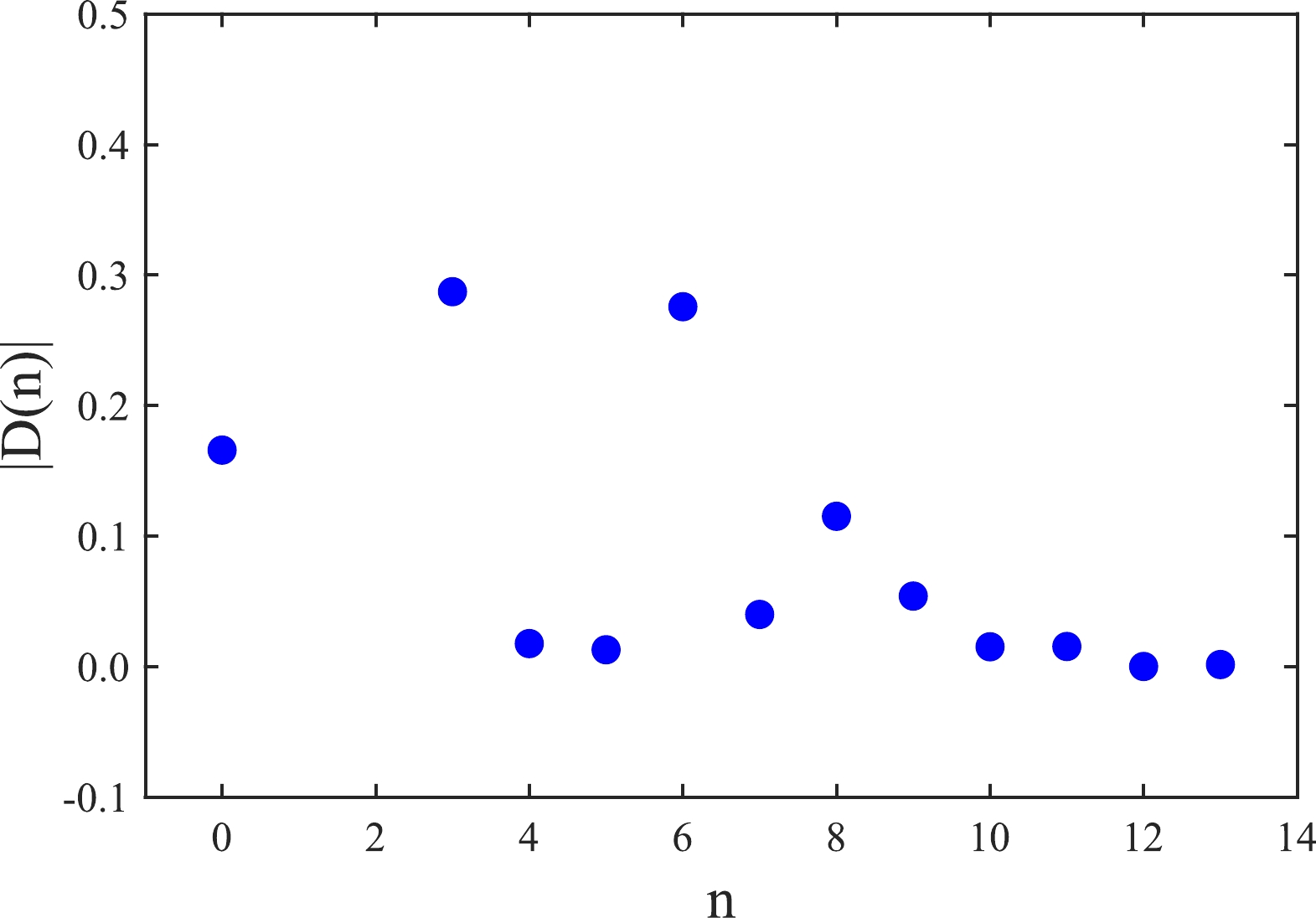
Figure 1. (color online) Absolute values of
$ D(n) $ with the central values of all the parameters for the$ \bar{D}\Xi_c $ molecular state with isospin$ (I,I_3)=(0,0) $ .In the last step, we take account of all uncertainties on the input parameters, including the quark masses, vacuum condensates, Borel parameters, and continuum threshold parameters, and acquire the masses and pole residues of hidden-charm molecular states without strange, with strange, and with double strange. These are presented explicitly in Table 2 and Figs. 2 and 3. From Tables 1 and 2, we can clearly see that the modified energy scale formula
$ \mu=\sqrt{M^2_{X/Y/Z/P}-(2{\mathbb{M}}_c)^2}-k\,\mathbb{M}_s $ with s-quark numbers$ k=0 $ ,$ 1 $ , and$ 2 $ is satisfied well [20]. In Figs. 2 and 3, we plot the masses of the$ \bar{D}\Xi_c $ and$ \bar{D}^*\Xi_c $ molecular states with the isospins$ (I,I_3)=(0,0) $ and$ (1,0) $ and variations of the Borel parameters at considerably larger ranges than the Borel windows, which are located between the two short perpendicular lines. Flat platforms are observed in the Borel windows, and the uncertainties originating from the Borel parameters can be safely ignored, which is congruous with the supplementary nature of$ T^2 $ . It is reliable to extract the molecule masses.$ (I,I_3) $ 

$M/\rm{GeV}$ 

$\lambda/ (10^{-3}\rm{GeV}^6)$ 

Thresholds/MeV Assignments $ \bar{D}\,\Xi_c $ 

$ (0,0) $ 

$ 4.34_{-0.07}^{+0.07} $ 

$ 1.43^{+0.19}_{-0.18} $ 

4337 ? $ P_{cs}(4338) $ 

$ \bar{D}\,\Xi_c $ 

$ (1,0) $ 

$ 4.46_{-0.07}^{+0.07} $ 

$ 1.37^{+0.19}_{-0.18} $ 

4337 $ \bar{D}\,\Lambda_c $ 

$(\dfrac{1}{2},\dfrac{1}{2})$ 

$ 4.46_{-0.08}^{+0.07} $ 

$ 1.47^{+0.20}_{-0.18} $ 

4151 $ \bar{D}_s\,\Xi_c $ 

$(\dfrac{1}{2},\dfrac{1}{2})$ 

$ 4.54_{-0.07}^{+0.07} $ 

$ 1.58^{+0.21}_{-0.20} $ 

4437 $ \bar{D}_s\,\Lambda_c $ 

$ (0,0) $ 

$ 4.48_{-0.07}^{+0.07} $ 

$ 1.57^{+0.21}_{-0.20} $ 

4255 $ \bar{D}^*\,\Xi_c $ 

$ (0,0) $ 

$ 4.46_{-0.07}^{+0.07} $ 

$ 1.55^{+0.20}_{-0.19} $ 

4479 ? $ P_{cs}(4459) $ 

$ \bar{D}^*\,\Xi_c $ 

$ (1,0) $ 

$ 4.63_{-0.08}^{+0.08} $ 

$ 1.69^{+0.22}_{-0.21} $ 

4479 $ \bar{D}^*\,\Lambda_c $ 

$(\dfrac{1}{2},\dfrac{1}{2})$ 

$ 4.59_{-0.08}^{+0.08} $ 

$ 1.67^{+0.22}_{-0.21} $ 

4293 $ \bar{D}^*_s\,\Xi_c $ 

$(\dfrac{1}{2},\dfrac{1}{2})$ 

$ 4.65_{-0.08}^{+0.08} $ 

$ 1.66^{+0.22}_{-0.21} $ 

4580 $ \bar{D}^*_s\,\Lambda_c $ 

$ (0,0) $ 

$ 4.50_{-0.07}^{+0.07} $ 

$ 1.52^{+0.21}_{-0.19} $ 

4398 Table 2. Masses and pole residues of pentaquark molecular states with possible assignments.
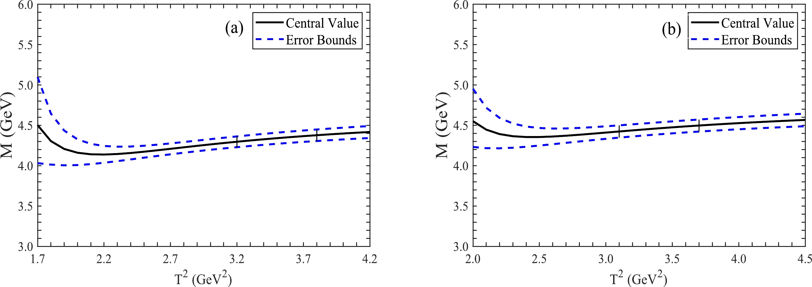
Figure 2. (color online) Masses of the
$ \bar{D}\Xi_c $ molecular states with variations of the Borel parameters$ T^2 $ , where (a) and (b) denote the isospins$ (0,0) $ and$ (1,0) $ , respectively.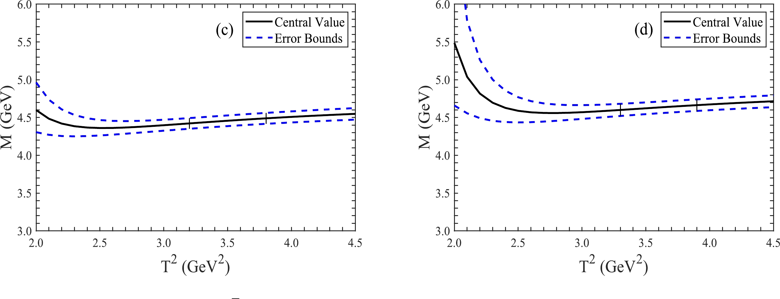
Figure 3. (color online) Masses of the
$ \bar{D}^{*}\Xi_c $ molecular states with variations of the Borel parameters$ T^2 $ , where (c) and (d) denote the isospins$ (0,0) $ and$ (1,0) $ , respectively.Our investigations with the same constraints indicate that there may be
$ \bar{D}\Xi_c $ and$ \bar{D}^*\Xi_c $ molecular states with isospin$ (I,I_3)=(0,0) $ that lie near (irrespective of slightly above or below) the corresponding charmed meson-baryon thresholds, respectively. Conversely, the$ \bar{D}\Xi_c $ and$ \bar{D}^*\Xi_c $ molecular states with isospin$ (I,I_3)=(1,0) $ , the$ \bar{D}\Lambda_c $ ,$ \bar{D}_s\Xi_c $ ,$ \bar{D}^*\Lambda_c $ , and$ \bar{D}_s^*\Xi_c $ molecular states with isospin$(I,I_3)=(\dfrac{1}{2},\dfrac{1}{2})$ , and the$ \bar{D}_s\Lambda_c $ and$ \bar{D}^*_s\Lambda_c $ molecular states with isospin$ (I,I_3)=(0,0) $ lie above the corresponding charmed meson-baryon thresholds. These might be the charmed meson-baryon resonances and would have considerably larger widths than$ P_{cs}(4338) $ and$ P_{cs}(4459) $ .Our investigations favor identifying
$ P_{cs}(4338) $ as the$ \bar{D}\Xi_c $ molecular state with the spin-parity$J^P={\dfrac{1}{2}}^-$ and isospin$ I=0 $ . The observation of its cousin with isospin$ I=1 $ in the$ J/\psi\Sigma^0/\eta_c\Sigma^0 $ invariant mass distributions would decipher the inner structure of$ P_{cs}(4338) $ and lead to a more robust assignment. This study also favors identifying$ P_{cs}(4459) $ as the$ \bar{D}^*\Xi_c $ molecular state with the spin-parity$J^P={\dfrac{3}{2}}^-$ and isospin$ I=0 $ . In Ref. [27], we obtain the mass$ M=4.45\pm0.12\,\rm{GeV} $ for the$ \bar{D}\,\Xi_c^{\prime} $ molecular state with$J^P={\dfrac{1}{2}}^-$ and$ M=4.51\pm0.11\,\rm{GeV} $ for the$ \bar{D}\,\Xi_c^{*} $ molecular state with$J^P={\dfrac{3}{2}}^-$ , which favor identifying$ P_{cs}(4459) $ as the$ \bar{D}\Xi^\prime_c $ molecular state with the spin-parity$J^P={\dfrac{1}{2}}^-$ and isospin$ I=0 $ . Currently, we cannot exclude the possibility of identifying$ P_{cs}(4459) $ as the$ \bar{D}\Xi^*_c $ molecular state with the spin-parity$J^P={\dfrac{3}{2}}^-$ and isospin$ I=0 $ considering the uncertainty on the mass. Precise measurement of the mass and more experimental data on the quantum numbers, such as the spin and parity, are still needed. Furthermore, the observation of the cousin of$ P_{cs}(4459) $ with isospin$ I=1 $ in the$ J/\psi\Sigma^0/\eta_c\Sigma^0 $ invariant mass distributions is of crucial importance and would decipher the inner structure of$ P_{cs}(4459) $ , leading to a more robust assignment. -
In this study, we extend our previous studies on pentaquark (molecular) states and distinguish the isospins of the interpolating currents to investigate in detail the
$ \bar{D}\,\Xi_c $ ,$ \bar{D}\,\Lambda_c $ ,$\bar{D}_s\,\Xi_c,$ $ \bar{D}_s\,\Lambda_c $ ,$ \bar{D}^*\,\Xi_c $ ,$ \bar{D}^*\,\Lambda_c $ ,$ \bar{D}^*_s\,\Xi_c $ , and$ \bar{D}^*_s\,\Lambda_c $ molecular states without strange, with strange, and with double strange in the framework of QCD sum rules. Here, D,$ D_s $ ,$ D^* $ , and$ D_s^* $ represent color-singlet clusters having the same quantum numbers as physical mesons, and$ \Lambda_c $ and$ \Xi_c $ represent color-singlet clusters having the same quantum numbers as physical ground state flavor-antitriplet charmed baryons. Because charmed baryons in flavor antitriplets have smaller masses than those in flavor sextets with the same valence quarks, we expect to acquire the lowest molecular states (to be more precise, color-singlet-color-singlet type pentaquark states).We consistently accomplish operator product expansion up to the vacuum condensates of dimension
$ 13 $ and choose the best energy scales of the QCD spectral densities with the help of the modified energy scale formula, which plays a crucial role in matching the two fundamental criteria of the QCD sum rules. We acquire the masses and pole residues of these molecular states. Our investigation favors identifying$ P_{cs}(4338) $ ($ P_{cs}(4459) $ ) as the$ \bar{D}\Xi_c $ ($ \bar{D}^*\Xi_c $ ) molecular state with the spin-parity$J^P={\dfrac{1}{2}}^-$ (${\dfrac{3}{2}}^-$ ) and isospin$ (I,I_3)=(0,0) $ , which are in congruous with the decays into the final states$ J/\psi\Lambda $ . The observation of their cousins with isospin$ (I,I_3)=(1,0) $ in the$ J/\psi\Sigma^0/\eta_c\Sigma^0 $ invariant mass distributions would decipher the inner structures of$ P_{cs}(4338) $ and$ P_{cs}(4459) $ and lead to more robust assignments. Conversely, in the picture of diquark-diquark-antiquark type pentaquark states,$ P_{cs}(4338) $ cannot find its position, and$ P_{cs}(4459) $ can be tentatively identified as the strange partner of$ P_{c}(4312) $ .More experimental data are still required to reach final assignments. Furthermore, we make predictions for other pentaquark molecular states with the isospins
$(I,I_3)=(\dfrac{1}{2},\dfrac{1}{2})$ and$ (0,0) $ , which lie above the corresponding charmed meson-baryon thresholds. It is better to refer to these as resonances, and they would have considerably larger widths than$ P_{cs}(4338) $ and$ P_{cs}(4459) $ . All the predictions can be confronted to experimental data in the future. -
Detailed QCD spectral densities for the current
$ J_{(0,0)}^{\bar{D}\Xi_c}(x) $ are$ \begin{aligned}[b] \rho_{\rm QCD}^1(s)=&\sum\limits_{n}\Big[\rho^1_{a}(n)+\rho^1_{b}(n)\\&+\rho^1_{c}(n)\delta(s-\widetilde{m}_c^2)+\rho^1_{d}(n) \delta(s-\overline{m}_c^2)\Big]\, ,\\ \rho_{\rm QCD}^0(s)=&\sum\limits_{n}\Big[\rho^0_{a}(n)+\rho^0_{b}(n)\\&+\rho^0_{c}(n)\delta(s-\widetilde{m}_c^2)+ \rho^0_{d}(n)\delta(s-\overline{m}_c^2)\Big]\, , \end{aligned} $

where a, b, c, and d refer to four types of integrals, and n represents the dimension of the condensates. In these integrals, we introduce the notations
$ \widetilde{m}_c^2=\dfrac{m_c^2}{y(1-y)} $ ,$ \overline{m}_c^2=\dfrac{(y+z)m_c^2}{y z} $ ,$ \xi=y+z-1 $ ,$ \zeta=1-y $ , and$ \omega=s-\overline{m}_c^2 $ . For types a and b,$ y_i=\dfrac{1}{2}\left(1-\sqrt{1-4m_c^2/s}\right) $ ,$ y_f=\dfrac{1}{2}\Big(1+ \sqrt{1-4m_c^2/s}\Big) $ , and$ z_i=\dfrac{y m_c^2}{y s-m_c^2} $ . For types c and d,$ y_i=0 $ ,$ y_f=1 $ , and$ z_i=0 $ .The a type integrals are
$ \begin{aligned}[b]\\[-7pt] \rho^1_a(8)=\frac{m_s m_c \left[ 9 \langle\bar{q}g_s\sigma Gq\rangle \langle\bar{s}s\rangle-39 \langle\bar{q}q\rangle \langle\bar{q}g_s\sigma Gq\rangle + 7 \langle\bar{q}q\rangle \langle\bar{s}g_s\sigma Gs\rangle\right]}{9216\pi^4} \int_{y_i}^{y_f}{\rm d}y \, \zeta \, , \end{aligned} $ 
$\begin{aligned}[b] \rho^1_a(9)=& -\frac{13 m_c \langle\bar{s}s\rangle \langle\bar{q}q\rangle^2}{1152\pi^2} \int_{y_i}^{y_f}{\rm d}y \, \zeta-\frac{m_c g_s^2 \langle\bar{q}q\rangle \left[7 \langle\bar{q}q\rangle^2 + \langle\bar{q}q\rangle \langle\bar{s}s\rangle + 7 \langle\bar{s}s\rangle^2\right]}{62208\pi^4} \int_{y_i}^{y_f}{\rm d}y \, \zeta \\&+\frac{ m_s \langle\bar{s}s\rangle \langle\bar{q}q\rangle^2}{768\pi^2} \int_{y_i}^{y_f}{\rm d}y \, \zeta y -\frac{m_s g_s^2 \langle\bar{q}q\rangle^2 \left[14 \langle\bar{q}q\rangle - 13 \langle\bar{s}s\rangle\right]}{41472\pi^4} \int_{y_i}^{y_f}{\rm d}y \, \zeta y \, , \end{aligned} $

$ \rho^1_a(10)= \frac{11 \langle\bar{q}g_s\sigma Gq\rangle \langle\bar{s}g_s\sigma Gs\rangle}{8192\pi^4}\int_{y_i}^{y_f}{\rm d}y \, \zeta y +\frac{\langle g_s^2GG\rangle \langle\bar{q}q\rangle \left[\langle\bar{q}q\rangle + 14 \langle\bar{s}s\rangle\right]}{36864\pi^4} \int_{y_i}^{y_f}{\rm d}y \, \zeta y \, , $

$ \rho^0_a(8)=- \frac{m_s m_c^2 \left[39 \langle\bar{q}q\rangle \langle\bar{q}g_s\sigma Gq\rangle - 9 \langle\bar{q}g_s\sigma Gq\rangle \langle\bar{s}s\rangle - 7 \langle\bar{q}q\rangle \langle\bar{s}g_s\sigma Gs\rangle\right]}{9216\pi^4} \int_{y_i}^{y_f}{\rm d}y \, , $

$ \begin{aligned}[b] \rho^0_a(9) =&- \frac{13 m_c^2\langle\bar{q}q\rangle^2 \langle\bar{s}s\rangle}{1152\pi^2} \int_{y_i}^{y_f}{\rm d}y - \frac{m_c^2 g_s^2 \langle\bar{q}q\rangle \left[7 \langle\bar{q}q\rangle^2 + \langle\bar{q}q\rangle \langle\bar{s}s\rangle + 7 \langle\bar{s}s\rangle^2\right]}{62208\pi^4} \int_{y_i}^{y_f}{\rm d}y \\ &+ \frac{ m_s m_c \langle\bar{q}q\rangle^2 \langle\bar{s}s\rangle}{1152\pi^2} \int_{y_i}^{y_f}{\rm d}y \, y + \frac{m_s m_c g_s^2 \langle\bar{q}q\rangle^2 \left[-14 \langle\bar{q}q\rangle + 13 \langle\bar{s}s\rangle\right]}{62208\pi^4} \int_{y_i}^{y_f}{\rm d}y \,y \, , \end{aligned} $

$ \rho^0_a(10)= \frac{11 m_c \langle\bar{q}g_s\sigma Gq\rangle \langle\bar{s}g_s\sigma Gs\rangle}{12288\pi^4} \int_{y_i}^{y_f}{\rm d}y \,y + \frac{m_c\langle g_s^2GG\rangle \langle\bar{q}q\rangle \left[\langle\bar{q}q\rangle + 14 \langle\bar{s}s\rangle\right]}{55296\pi^4} \int_{y_i}^{y_f}{\rm d}y \, y \, . $

The b type integrals are
$ \rho_b^1(0)= \frac{13}{1572864 \pi^8} \int_{y_i}^{y_f}{\rm d}y\int_{z_i}^{\zeta}{\rm d}z \,y z \xi^4 \left(\frac{3\omega^5}{5}+s \omega^4\right) - \frac{ m_s m_c}{393216\pi^8} \int_{y_i}^{y_f}{\rm d}y\int_{z_i}^{\zeta}{\rm d}z \, z \xi^3\omega^4 \, , $

$ \rho_b^1(3)= -\frac{m_c \left[14 \langle\bar{q}q\rangle + \langle\bar{s}s\rangle\right]}{24576 \pi^6 } \int_{y_i}^{y_f}{\rm d}y\int_{z_i}^{\zeta}{\rm d}z \,z \xi^2\omega^3 + \frac{m_s\left[13 \langle\bar{s}s\rangle-28 \langle\bar{q}q\rangle\right]}{16384 \pi^6} \int_{y_i}^{y_f}{\rm d}y\int_{z_i}^{\zeta}{\rm d}z \,y z \xi^2\left(s+\omega\right) \omega^2 \, , $

$ \begin{aligned}[b] \rho_b^1(4)=& -\frac{13 m_c^2\langle g_s^2GG\rangle}{786432 \pi^8} \int_{y_i}^{y_f}{\rm d}y\int_{z_i}^{\zeta}{\rm d}z \,\frac{z \xi^4}{y^2} \left(\omega^2+\frac{2 s \omega}{3}\right)- \frac{29 \langle g_s^2GG\rangle}{1572864 \pi^8 } \int_{y_i}^{y_f}{\rm d}y\int_{z_i}^{\zeta}{\rm d}z \, z \xi^3 \left(\omega^3+s \omega^2\right)\\ &+ \frac{\langle g_s^2GG\rangle}{32768\pi^8} \int_{y_i}^{y_f}{\rm d}y\int_{z_i}^{\zeta}{\rm d}z \, y z \xi^2 \left(\omega^3+s \omega^2\right) + \frac{m_s m_c^3 \langle g_s^2GG\rangle}{1179648 \pi^8 } \int_{y_i}^{y_f}{\rm d}y\int_{z_i}^{\zeta}{\rm d}z \, \frac{\xi^3\omega}{y^2} \\ &+\frac{m_s m_c \langle g_s^2GG\rangle}{786432\pi^8} \int_{y_i}^{y_f}{\rm d}y\int_{z_i}^{\zeta}{\rm d}z \, \frac{z \xi^3}{y^2} \left(y \omega^2+\frac{2 s y \omega}{3}-\frac{2 \omega^2}{3}\right) + \frac{m_s m_c \langle g_s^2GG\rangle}{131072\pi^8} \int_{y_i}^{y_f}{\rm d}y\int_{z_i}^{\zeta}{\rm d}z \left(\frac{z \xi^2\omega^2}{y}-z \xi\omega^2\right) \, , \end{aligned} $

$ \begin{aligned}[b] \rho_b^1(5)=& -\frac{m_c \langle\bar{q}g_s\sigma Gq\rangle}{16384\pi^6} \int_{y_i}^{y_f}{\rm d}y\int_{z_i}^{\zeta}{\rm d}z \left(11 z \xi\omega^2+\frac{14 z \xi^2\omega^2}{y}\right) \\&+ \frac{ m_s}{24576\pi^6} \left[-36 \langle\bar{q}g_s\sigma Gq\rangle + 13 \langle\bar{s}g_s\sigma Gs\rangle\right] \int_{y_i}^{y_f}{\rm d}y\int_{z_i}^{\zeta}{\rm d}z \, y z \xi \left(\frac{3 \omega^2}{2}+s \omega\right)\\ &- \frac{m_s \langle\bar{q}g_s\sigma Gq\rangle}{8192\pi^6} \int_{y_i}^{y_f}{\rm d}y\int_{z_i}^{\zeta}{\rm d}z \, z \xi^2 \left(\frac{3 \omega^2}{2}+s \omega\right)\, , \end{aligned} $

$ \begin{aligned}[b] \rho_b^1(6)=& -\frac{\langle\bar{q}q\rangle\left[\langle\bar{q}q\rangle+14\langle\bar{s}s\rangle\right]}{1024\pi^4} \int_{y_i}^{y_f}{\rm d}y\int_{z_i}^{\zeta}{\rm d}z \, y z \xi \left(\frac{2 s \omega}{3 }+ \omega^2\right) -\frac{13\left[2 g_s^2 \langle\bar{q}q\rangle^2+ g_s^2 \langle\bar{s}s\rangle^2\right]}{110592\pi^6} \int_{y_i}^{y_f}{\rm d}y\int_{z_i}^{\zeta}{\rm d}z \, y z \xi \left(\frac{2 s \omega}{3 }+ \omega^2\right)\\ &+ \frac{ m_s m_c \langle\bar{q}q\rangle \left[13 \langle\bar{q}q\rangle - 7 \langle\bar{s}s\rangle\right]}{1536\pi^4} \int_{y_i}^{y_f}{\rm d}y\int_{z_i}^{\zeta}{\rm d}z \,z\omega + \frac{ m_s m_c g_s^2 \langle\bar{q}q\rangle^2}{82944\pi^6} \int_{y_i}^{y_f}{\rm d}y\int_{z_i}^{\zeta}{\rm d}z \,z\omega \, , \end{aligned} $

$ \begin{aligned}[b] \rho_b^1(7)=& \frac{m_c^3 \langle g_s^2GG\rangle \left[14 \langle\bar{q}q\rangle + \langle\bar{s}s\rangle\right]}{294912 \pi^6 } \int_{y_i}^{y_f}{\rm d}y\int_{z_i}^{\zeta}{\rm d}z \, \frac{\xi^2}{y^2}+ \frac{m_c\langle g_s^2GG\rangle \left[14 \langle\bar{q}q\rangle + \langle\bar{s}s\rangle\right]}{98304\pi^6} \int_{y_i}^{y_f}{\rm d}y\int_{z_i}^{\zeta}{\rm d}z \, \frac{z \xi^2}{y^2} \left(y \omega-\frac{2\omega}{3}+\frac{s y}{3}\right)\\ &+ \frac{m_c\langle g_s^2GG\rangle \left[3 \langle\bar{q}q\rangle + 2 \langle\bar{s}s\rangle\right]}{49152\pi^6} \int_{y_i}^{y_f}{\rm d}y\int_{z_i}^{\zeta}{\rm d}z \, \frac{z \xi\omega}{y} -\frac{m_c\langle g_s^2GG\rangle \left[56 \langle\bar{q}q\rangle + 7\langle\bar{s}s\rangle\right]}{294912\pi^6} \int_{y_i}^{y_f}{\rm d}y\int_{z_i}^{\zeta}{\rm d}z \, z\omega\\ &- \frac{m_s m_c^2 \langle g_s^2GG\rangle \left[-28 \langle\bar{q}q\rangle + 13 \langle\bar{s}s\rangle\right]}{98304\pi^6} \int_{y_i}^{y_f}{\rm d}y\int_{z_i}^{\zeta}{\rm d}z \, \frac{z \xi^2}{y^2} +\frac{7 m_s\langle g_s^2GG\rangle \left[2 \langle\bar{q}q\rangle - \langle\bar{s}s\rangle\right]}{49152\pi^6} \int_{y_i}^{y_f}{\rm d}y\int_{z_i}^{\zeta}{\rm d}z \, z \xi \left(s+3 \omega\right)\\ &+ \frac{ m_s \langle g_s^2GG\rangle \left[3\langle\bar{s}s\rangle-14\langle\bar{q}q\rangle\right]}{294912\pi^6} \int_{y_i}^{y_f}{\rm d}y\int_{z_i}^{\zeta}{\rm d}z \, y z \left(s +3 \omega\right)\, , \end{aligned} $

$ \begin{aligned}[b] \rho_b^1(8)=& -\frac{12 \langle\bar{q}g_s\sigma Gq\rangle \langle\bar{s}s\rangle + \langle\bar{q}q\rangle \left[\langle\bar{q}g_s\sigma Gq\rangle + 13 \langle\bar{s}g_s\sigma Gs\rangle\right]}{6144\pi^4} \int_{y_i}^{y_f}{\rm d}y\int_{z_i}^{\zeta}{\rm d}z \, y z \left(s+3 \omega\right)\\ & -\frac{2 \langle\bar{q}g_s\sigma Gq\rangle \langle\bar{s}s\rangle + \langle\bar{q}q\rangle \left[2 \langle\bar{q}g_s\sigma Gq\rangle + \langle\bar{s}g_s\sigma Gs\rangle\right]}{6144\pi^4} \int_{y_i}^{y_f}{\rm d}y\int_{z_i}^{\zeta}{\rm d}z \, z \xi \left(s+3 \omega\right)\\ &+ \frac{7 m_s m_c \langle\bar{q}g_s\sigma Gq\rangle \left[2 \langle\bar{q}q\rangle - \langle\bar{s}s\rangle\right]}{3072\pi^4} \int_{y_i}^{y_f}{\rm d}y\int_{z_i}^{\zeta}{\rm d}z \, \frac{z}{y}\, , \end{aligned} $

$ \begin{aligned}[b] \rho_b^1(10)= \frac{\langle g_s^2GG\rangle \langle\bar{q}q\rangle \left[\langle\bar{q}q\rangle + 20 \langle\bar{s}s\rangle\right]}{24576\pi^4} \int_{y_i}^{y_f}{\rm d}y\int_{z_i}^{\zeta}{\rm d}z \,z - \frac{\langle\bar{q}g_s\sigma Gq\rangle \left[24 \langle\bar{q}g_s\sigma Gq\rangle + 35 \langle\bar{s}g_s\sigma Gs\rangle\right]}{196608\pi^4} \int_{y_i}^{y_f}{\rm d}y\int_{z_i}^{\zeta}{\rm d}z \, z \, , \end{aligned} $

$ \rho_b^0(0)= \frac{13 m_c}{1572864 \pi^8} \int_{y_i}^{y_f}{\rm d}y\int_{z_i}^{\zeta}{\rm d}z \, y \xi^4 \left(\frac{2 \omega^5}{5}+s \omega^4\right)- \frac{ m_s m_c^2}{393216\pi^8} \int_{y_i}^{y_f}{\rm d}y\int_{z_i}^{\zeta}{\rm d}z \, \xi^3\omega^4 \, , $

$ \rho_b^0(3)= -\frac{m_c^2 \left[14 \langle\bar{q}q\rangle + \langle\bar{s}s\rangle\right]}{24576\pi^6} \int_{y_i}^{y_f}{\rm d}y\int_{z_i}^{\zeta}{\rm d}z \, \xi^2\omega^3 - \frac{m_c m_s \left[28 \langle\bar{q}q\rangle - 13 \langle\bar{s}s\rangle\right]}{16384\pi^6} \int_{y_i}^{y_f}{\rm d}y\int_{z_i}^{\zeta}{\rm d}z \, y \xi^2 \left(\frac{2\omega^3}{3}+s \omega^2\right)\, , $

$ \begin{aligned}[b] \rho_b^0(4)=& -\frac{13 m_c^3 \langle g_s^2GG\rangle}{4718592\pi^8} \int_{y_i}^{y_f}{\rm d}y\int_{z_i}^{\zeta}{\rm d}z \, \frac{\xi^4}{y^2} \left(\omega^2+s \omega\right)-\frac{13 m_c \langle g_s^2GG\rangle}{4718592\pi^8} \int_{y_i}^{y_f}{\rm d}y\int_{z_i}^{\zeta}{\rm d}z \, \frac{z \xi^4}{y^2} \left(s^2 y \omega+y \omega^3-s \omega^2\right)\\ & -\frac{13 m_c \langle g_s^2GG\rangle}{1572864\pi^8} \int_{y_i}^{y_f}{\rm d}y\int_{z_i}^{\zeta}{\rm d}z \, \frac{z \xi^4}{y^2} \left(s y \omega^2-\frac{2\omega^3}{9}\right)- \frac{29 m_c \langle g_s^2GG\rangle}{1572864\pi^8} \int_{y_i}^{y_f}{\rm d}y\int_{z_i}^{\zeta}{\rm d}z \, \xi^3 \left(\frac{2\omega^3}{3}+s \omega^2\right)\\ &+ \frac{ m_c \langle g_s^2GG\rangle}{32768\pi^8} \int_{y_i}^{y_f}{\rm d}y\int_{z_i}^{\zeta}{\rm d}z \, y \xi^2 \left(\frac{2\omega^3}{3}+s \omega^2\right) -\frac{m_s m_c^2 \langle g_s^2GG\rangle}{589824\pi^8} \int_{y_i}^{y_f}{\rm d}y\int_{z_i}^{\zeta}{\rm d}z \, \frac{\xi^3}{y^2} \left(\zeta \omega^2-s y \omega\right)\\ &+ \frac{m_s m_c^2 \langle g_s^2GG\rangle}{131072\pi^8} \int_{y_i}^{y_f}{\rm d}y\int_{z_i}^{\zeta}{\rm d}z \left(\frac{\xi^2\omega^2}{y}-\xi\omega^2\right) \, , \end{aligned} $

$ \begin{aligned}[b] \rho_b^0(5)=& -\frac{m_c^2 \left[14 \langle\bar{q}g_s\sigma Gq\rangle + \langle\bar{s}g_s\sigma Gs\rangle\right]}{16384\pi^6} \int_{y_i}^{y_f}{\rm d}y\int_{z_i}^{\zeta}{\rm d}z \, \xi\omega^2 - \frac{7 m_c^2 \langle\bar{q}g_s\sigma Gq\rangle}{8192\pi^6} \int_{y_i}^{y_f}{\rm d}y\int_{z_i}^{\zeta}{\rm d}z \, \frac{\xi^2\omega^2}{y} \\ &+ \frac{m_c^2 \left[3 \langle\bar{q}g_s\sigma Gq\rangle + \langle\bar{s}g_s\sigma Gs\rangle\right]}{16384\pi^6} \int_{y_i}^{y_f}{\rm d}y\int_{z_i}^{\zeta}{\rm d}z \, \xi\omega^2- \frac{m_s m_c \left[42 \langle\bar{q}g_s\sigma Gq\rangle - 13 \langle\bar{s}g_s\sigma Gs\rangle\right]}{24576\pi^6} \int_{y_i}^{y_f}{\rm d}y\int_{z_i}^{\zeta}{\rm d}z \, y \xi \left(\omega^2+s \omega\right)\\ & -\frac{m_s m_c\langle\bar{q}g_s\sigma Gq\rangle}{8192\pi^6} \int_{y_i}^{y_f}{\rm d}y\int_{z_i}^{\zeta}{\rm d}z \, \xi^2 \left(\omega^2+s \omega\right)+\frac{m_s m_c \langle\bar{q}g_s\sigma Gq\rangle}{4096\pi^6} \int_{y_i}^{y_f}{\rm d}y\int_{z_i}^{\zeta}{\rm d}z \, y \xi \left(\omega^2+s \omega\right)\, , \end{aligned} $

$ \begin{aligned}[b] \rho_b^0(6)=& -\frac{m_c \langle\bar{q}q\rangle \left[\langle\bar{q}q\rangle + 14 \langle\bar{s}s\rangle\right]}{1536\pi^4} \int_{y_i}^{y_f}{\rm d}y\int_{z_i}^{\zeta}{\rm d}z \, y \xi \left(\omega^2+s \omega\right)\\ &+ \frac{m_s m_c^2 \langle\bar{q}q\rangle \left[13 \langle\bar{q}q\rangle - 7 \langle\bar{s}s\rangle\right]}{1536\pi^4} \int_{y_i}^{y_f}{\rm d}y\int_{z_i}^{\zeta}{\rm d}z \, \omega+ \frac{m_s m_c^2 g_s^2 \langle\bar{q}q\rangle^2}{82944\pi^6} \int_{y_i}^{y_f}{\rm d}y\int_{z_i}^{\zeta}{\rm d}z \, \omega\\ & -\frac{13 m_c \left[2 g_s^2 \langle\bar{q}q\rangle^2 + g_s^2 \langle\bar{s}s\rangle^2\right]}{165888\pi^6} \int_{y_i}^{y_f}{\rm d}y\int_{z_i}^{\zeta}{\rm d}z \, y \xi \left(\omega^2+s \omega\right)\, , \end{aligned} $

$ \begin{aligned}[b] \rho_b^0(7)=& \frac{m_c^2\langle g_s^2GG\rangle \left[14 \langle\bar{q}q\rangle + \langle\bar{s}s\rangle\right]}{73728\pi^6} \int_{y_i}^{y_f}{\rm d}y\int_{z_i}^{\zeta}{\rm d}z \, \frac{\xi^2}{y^2} \left(-\zeta\omega+\frac{s y}{2}\right)+ \frac{m_c^2\langle g_s^2GG\rangle \left[3 \langle\bar{q}q\rangle + 2 \langle\bar{s}s\rangle\right]}{49152\pi^6} \int_{y_i}^{y_f}{\rm d}y\int_{z_i}^{\zeta}{\rm d}z \, \frac{\xi\omega}{y}\\ & -\frac{7m_c^2\langle g_s^2GG\rangle \left[8 \langle\bar{q}q\rangle + \langle\bar{s}s\rangle\right]}{294912\pi^6} \int_{y_i}^{y_f}{\rm d}y\int_{z_i}^{\zeta}{\rm d}z \, \omega+ \frac{ m_s m_c^3\langle g_s^2GG\rangle \left[28 \langle\bar{q}q\rangle - 13 \langle\bar{s}s\rangle\right]}{294912\pi^6} \int_{y_i}^{y_f}{\rm d}y\int_{z_i}^{\zeta}{\rm d}z \left(\frac{\xi^2}{y^2}+\frac{z \xi^2}{y^3}\right) \\ &- \frac{m_s m_c\langle g_s^2GG\rangle \left[28 \langle\bar{q}q\rangle - 13 \langle\bar{s}s\rangle\right]}{196608\pi^6} \int_{y_i}^{y_f}{\rm d}y\int_{z_i}^{\zeta}{\rm d}z \, \frac{z \xi^2}{y^2} \left(s +2\omega\right)+ \frac{7 m_s m_c\langle g_s^2GG\rangle \left[2 \langle\bar{q}q\rangle - \langle\bar{s}s\rangle\right]}{49152\pi^6} \int_{y_i}^{y_f}{\rm d}y\int_{z_i}^{\zeta}{\rm d}z \, \xi \left(s+2\omega\right)\\ &+\frac{ m_s m_c \langle g_s^2GG\rangle \langle\bar{s}s\rangle}{98304\pi^6} \int_{y_i}^{y_f}{\rm d}y\int_{z_i}^{\zeta}{\rm d}z \, y \left(s+2\omega\right)- \frac{7 m_s m_c \langle g_s^2GG\rangle \langle\bar{q}q\rangle}{147456\pi^6} \int_{y_i}^{y_f}{\rm d}y\int_{z_i}^{\zeta}{\rm d}z \, y \left(s+2\omega\right)\, , \end{aligned} $

$ \begin{aligned}[b] \rho_b^0(8)=& -\frac{ m_c \left\{7 \langle\bar{q}g_s\sigma Gq\rangle \langle\bar{s}s\rangle + \langle\bar{q}q\rangle \left[\langle\bar{q}g_s\sigma Gq\rangle + 7 \langle\bar{s}g_s\sigma Gs\rangle\right]\right\}}{3072\pi^4} \int_{y_i}^{y_f}{\rm d}y\int_{z_i}^{\zeta}{\rm d}z \left(s y+2y\omega\right)\\ & -\frac{m_c\left\{2 \langle\bar{q}g_s\sigma Gq\rangle \langle\bar{s}s\rangle + \langle\bar{q}q\rangle \left[2 \langle\bar{q}g_s\sigma Gq\rangle + \langle\bar{s}g_s\sigma Gs\rangle\right]\right\}}{6144\pi^4} \int_{y_i}^{y_f}{\rm d}y\int_{z_i}^{\zeta}{\rm d}z \left(\xi s+2\xi\omega\right)\\ & +\frac{m_c\left\{2 \langle\bar{q}g_s\sigma Gq\rangle \langle\bar{s}s\rangle + \langle\bar{q}q\rangle \left[\langle\bar{q}g_s\sigma Gq\rangle + \langle\bar{s}g_s\sigma Gs\rangle\right]\right\}}{6144\pi^4} \int_{y_i}^{y_f}{\rm d}y\int_{z_i}^{\zeta}{\rm d}z \left(y s+2y\omega\right)\\ &- \frac{7 m_s m_c^2 \langle\bar{q}g_s\sigma Gq\rangle \left[-2 \langle\bar{q}q\rangle + \langle\bar{s}s\rangle\right]}{3072\pi^4} \int_{y_i}^{y_f}{\rm d}y\int_{z_i}^{\zeta}{\rm d}z \, \frac{1}{y}\, , \end{aligned} $

$ \begin{aligned}[b] \rho_b^0(10)=& \frac{m_c\langle g_s^2GG\rangle \langle\bar{q}q\rangle \left[\langle\bar{q}q\rangle + 14 \langle\bar{s}s\rangle\right]}{18432\pi^4} \int_{y_i}^{y_f}{\rm d}y\int_{z_i}^{\zeta}{\rm d}z \, \frac{z \xi}{y^2} \left(y-\frac{2}{3}\right)\\ &+ \frac{m_c \langle g_s^2GG\rangle \langle\bar{q}q\rangle \left[\langle\bar{q}q\rangle + 28 \langle\bar{s}s\rangle\right]}{36864\pi^4} \int_{y_i}^{y_f}{\rm d}y\int_{z_i}^{\zeta}{\rm d}z \\ &- \frac{m_c \langle\bar{q}g_s\sigma Gq\rangle \left[24 \langle\bar{q}g_s\sigma Gq\rangle + 35 \langle\bar{s}g_s\sigma Gs\rangle\right]}{294912\pi^4} \int_{y_i}^{y_f}{\rm d}y\int_{z_i}^{\zeta}{\rm d}z \, . \end{aligned} $

The c type integrals are
$ \rho_c^1(9)= - \frac{m_s g_s^2 \langle\bar{q}q\rangle^2 \left[14 \langle\bar{q}q\rangle - 13 \langle\bar{s}s\rangle\right]}{124416\pi^4} \int_{y_i}^{y_f}{\rm d}y \, \zeta y\widetilde{m}_c^2+\frac{m_s \langle\bar{q}q\rangle^2 \langle\bar{s}s\rangle}{2304\pi^2} \int_{y_i}^{y_f}{\rm d}y \, \zeta y\widetilde{m}_c^2 \, , $

$ \begin{aligned}[b] \rho_c^1(10)=& \frac{11\langle\bar{q}g_s\sigma Gq\rangle \langle\bar{s}g_s\sigma Gs\rangle}{24576\pi^4} \int_{y_i}^{y_f}{\rm d}y \, \zeta y\widetilde{m}_c^2 + \frac{\langle g_s^2GG\rangle \langle\bar{q}q\rangle \left[\langle\bar{q}q\rangle + 14 \langle\bar{s}s\rangle\right]}{110592\pi^4} \int_{y_i}^{y_f}{\rm d}y \, \zeta y\widetilde{m}_c^2 \\ &- \frac{m_s m_c \langle\bar{q}g_s\sigma Gq\rangle \left[-39 \langle\bar{q}g_s\sigma Gq\rangle + 14 \langle\bar{s}g_s\sigma Gs\rangle\right]}{36864\pi^4} \int_{y_i}^{y_f}{\rm d}y \, \zeta \left(1+\frac{\widetilde{m}_c^2}{2 T^2}\right)\end{aligned} $

$ \begin{aligned}[b] \qquad\quad\quad&- \frac{m_s m_c \langle g_s^2GG\rangle \langle\bar{q}q\rangle \langle\bar{s}s\rangle}{36864\pi^4} \int_{y_i}^{y_f}{\rm d}y \, \frac{\zeta}{y} - \frac{m_s m_c \langle g_s^2GG\rangle \langle\bar{q}q\rangle \left[-26 \langle\bar{q}q\rangle + 7 \langle\bar{s}s\rangle\right]}{110592\pi^4} \int_{y_i}^{y_f}{\rm d}y \, \zeta \left(1+\frac{\widetilde{m}_c^2}{2 T^2}\right)\\ &- \frac{7 m_s m_c \langle\bar{q}g_s\sigma Gq\rangle \left[3 \langle\bar{q}g_s\sigma Gq\rangle - \langle\bar{s}g_s\sigma Gs\rangle\right]}{18432\pi^4} \int_{y_i}^{y_f}{\rm d}y \, \frac{\zeta}{y} \\ & +\frac{ m_s m_c \langle\bar{q}g_s\sigma Gq\rangle \langle\bar{s}g_s\sigma Gs\rangle}{18432\pi^4} \int_{y_i}^{y_f}{\rm d}y \, \zeta \left(1+\frac{\widetilde{m}_c^2}{2 T^2}\right) \, , \end{aligned} $

$ \begin{aligned}[b] \rho_c^1(11)=& \frac{13 m_c \langle\bar{q}q\rangle \left[2 \langle\bar{q}g_s\sigma Gq\rangle \langle\bar{s}s\rangle + \langle\bar{q}q\rangle \langle\bar{s}g_s\sigma Gs\rangle\right]}{2304\pi^2} \int_{y_i}^{y_f}{\rm d}y \, \zeta \left(1+\frac{\widetilde{m}_c^2}{2 T^2}\right)\\ &+ \frac{7 m_c \langle\bar{q}g_s\sigma Gq\rangle g_s^2 \langle\bar{s}s\rangle^2}{124416\pi^4} \int_{y_i}^{y_f}{\rm d}y \, \zeta \left(1+\frac{\widetilde{m}_c^2}{2 T^2}\right)\\ &- \frac{ m_c \langle\bar{q}q\rangle \left[28 \langle\bar{q}g_s\sigma Gq\rangle \langle\bar{s}s\rangle + \langle\bar{q}q\rangle \langle\bar{s}g_s\sigma Gs\rangle\right]}{4608\pi^2} \int_{y_i}^{y_f}{\rm d}y \, \frac{\zeta}{y} \\ &+ \frac{m_c g_s^2 \langle\bar{q}q\rangle^2 \left[7 \langle\bar{q}g_s\sigma Gq\rangle + \langle\bar{s}g_s\sigma Gs\rangle\right]}{124416\pi^4} \int_{y_i}^{y_f}{\rm d}y \, \zeta \left(1+\frac{\widetilde{m}_c^2}{2 T^2}\right)\\ &- \frac{m_s \langle\bar{q}q\rangle \left[3 \langle\bar{q}g_s\sigma Gq\rangle \langle\bar{s}s\rangle + \langle\bar{q}q\rangle \langle\bar{s}g_s\sigma Gs\rangle\right]}{6912\pi^2} \int_{y_i}^{y_f}{\rm d}y \, \zeta y \left(3+\frac{\widetilde{m}_c^4}{2 T^4}+\frac{2 \widetilde{m}_c^2}{ T^2}\right)\\ &+ \frac{m_s g_s^2 \langle\bar{q}q\rangle^2 \left[21 \langle\bar{q}g_s\sigma Gq\rangle - 13 \langle\bar{s}g_s\sigma Gs\rangle\right]}{373248\pi^4} \int_{y_i}^{y_f}{\rm d}y \, \zeta y \left(3+\frac{\widetilde{m}_c^4}{2 T^4}+\frac{2 \widetilde{m}_c^2}{ T^2}\right)\\ &+ \frac{ m_s \langle\bar{q}q\rangle \langle\bar{q}g_s\sigma Gq\rangle \langle\bar{s}s\rangle}{2304\pi^2} \int_{y_i}^{y_f}{\rm d}y \, \zeta \left(1+\frac{\widetilde{m}_c^2}{2 T^2}\right)\, , \end{aligned} $

$ \begin{aligned}[b] \rho_c^1(12)= \frac{ g_s^2 \langle\bar{q}q\rangle^2 \langle\bar{s}s\rangle \left[14 \langle\bar{q}q\rangle + \langle\bar{s}s\rangle\right]}{46656\pi^2} \int_{y_i}^{y_f}{\rm d}y \, \zeta y \left(3+\frac{\widetilde{m}_c^4}{2 T^4}+\frac{2 \widetilde{m}_c^2}{ T^2}\right)-\frac{7 m_s m_c g_s^2 \langle\bar{s}s\rangle \langle\bar{q}q\rangle^3}{93312\pi^2} \int_{y_i}^{y_f}{\rm d}y \, \zeta \left(\frac{\widetilde{m}_c^4}{ T^6}+\frac{2 \widetilde{m}_c^2}{ T^4}+\frac{2}{ T^2}\right) \, , \end{aligned} $

$ \begin{aligned}[b] \rho_c^1(13)=& -\frac{13 m_c \langle\bar{q}g_s\sigma Gq\rangle \left[\langle\bar{q}g_s\sigma Gq\rangle \langle\bar{s}s\rangle + 2 \langle\bar{q}q\rangle \langle\bar{s}g_s\sigma Gs\rangle\right]}{18432\pi^2} \int_{y_i}^{y_f}{\rm d}y \, \zeta \left(\frac{2}{ T^2}+\frac{2\widetilde{m}_c^2}{ T^4}+\frac{\widetilde{m}_c^4}{ T^6} \right)\\ &+ \frac{13 m_c^3 \langle g_s^2GG\rangle \langle\bar{q}q\rangle^2 \langle\bar{s}s\rangle}{82944\pi^2T^4} \int_{y_i}^{y_f}{\rm d}y \, \frac{1}{y^2} + \frac{13 m_c\langle g_s^2GG\rangle \langle\bar{q}q\rangle^2 \langle\bar{s}s\rangle }{41472\pi^2} \int_{y_i}^{y_f}{\rm d}y \, \frac{\zeta}{y^2} \left(\frac{\widetilde{m}_c^2 y}{2 T^4}-\frac{1}{ T^2}+\frac{y}{2 T^2}\right) \\ & -\frac{13 m_c \langle g_s^2GG\rangle \langle\bar{q}q\rangle^2 \langle\bar{s}s\rangle}{55296\pi^2} \int_{y_i}^{y_f}{\rm d}y \, \zeta\left(\frac{\widetilde{m}_c^4}{ T^6}+\frac{2 \widetilde{m}_c^2}{ T^4}+\frac{2}{ T^2}\right)\\ &+ \frac{m_c \langle\bar{q}g_s\sigma Gq\rangle \left[14 \langle\bar{q}g_s\sigma Gq\rangle \langle\bar{s}s\rangle + 15 \langle\bar{q}q\rangle \langle\bar{s}g_s\sigma Gs\rangle\right]}{9216\pi^2} \int_{y_i}^{y_f}{\rm d}y \, \frac{\zeta}{y} \left(\frac{\widetilde{m}_c^2}{T^4}+\frac{1}{ T^2}\right)\\ &+ \frac{m_s \langle\bar{q}g_s\sigma Gq\rangle \left[3 \langle\bar{q}g_s\sigma Gq\rangle \langle\bar{s}s\rangle + 4 \langle\bar{q}q\rangle \langle\bar{s}g_s\sigma Gs\rangle\right]}{110592\pi^2} \int_{y_i}^{y_f}{\rm d}y \, \zeta y \left(\frac{6 }{ T^2}+\frac{6 \widetilde{m}_c^2 }{ T^4}+\frac{3 \widetilde{m}_c^4}{ T^6}+\frac{ \widetilde{m}_c^6}{ T^8}\right)\\ & -\frac{m_s m_c^2 \langle g_s^2GG\rangle \langle\bar{q}q\rangle^2 \langle\bar{s}s\rangle}{82944\pi^2} \int_{y_i}^{y_f}{\rm d}y \, \frac{\zeta}{y^2} \frac{\widetilde{m}_c^2}{ T^6}\\ &+ \frac{m_s \langle g_s^2GG\rangle \langle\bar{q}q\rangle^2 \langle\bar{s}s\rangle}{165888\pi^2} \int_{y_i}^{y_f}{\rm d}y \, \zeta y \left(\frac{ \widetilde{m}_c^6}{ T^8}+\frac{3 \widetilde{m}_c^4}{ T^6}+\frac{6 \widetilde{m}_c^2}{ T^4}+\frac{6}{ T^2}\right) \\ &- \frac{m_s \langle\bar{q}g_s\sigma Gq\rangle \left[3 \langle\bar{q}g_s\sigma Gq\rangle \langle\bar{s}s\rangle + 2 \langle\bar{q}q\rangle \langle\bar{s}g_s\sigma Gs\rangle\right]}{27648\pi^2} \int_{y_i}^{y_f}{\rm d}y \, \zeta \left(\frac{\widetilde{m}_c^4}{2 T^6}+\frac{\widetilde{m}_c^2}{ T^4}+\frac{1}{ T^2}\right)\, , \end{aligned} $

$ \rho_c^0(9)= \frac{m_s m_c g_s^2 \langle\bar{q}q\rangle^2 \left[-14 \langle\bar{q}q\rangle + 13 \langle\bar{s}s\rangle\right]}{124416\pi^4} \int_{y_i}^{y_f}{\rm d}y \, y\widetilde{m}_c^2+\frac{m_s m_c \langle\bar{q}q\rangle^2 \langle\bar{s}s\rangle}{2304\pi^2} \int_{y_i}^{y_f}{\rm d}y \, y\widetilde{m}_c^2 \, , $

$ \begin{aligned}[b] \rho_c^0(10)=& \frac{11 m_c \langle\bar{q}g_s\sigma Gq\rangle \langle\bar{s}g_s\sigma Gs\rangle}{24576\pi^4} \int_{y_i}^{y_f}{\rm d}y \, y\widetilde{m}_c^2 + \frac{m_c\langle g_s^2GG\rangle \langle\bar{q}q\rangle \left[\langle\bar{q}q\rangle + 14 \langle\bar{s}s\rangle\right]}{110592\pi^4} \int_{y_i}^{y_f}{\rm d}y \, y\widetilde{m}_c^2 \\ &+ \frac{m_s m_c^2 \langle\bar{q}g_s\sigma Gq\rangle \left[39 \langle\bar{q}g_s\sigma Gq\rangle - 14 \langle\bar{s}g_s\sigma Gs\rangle\right]}{73728\pi^4} \int_{y_i}^{y_f}{\rm d}y \left(1+\frac{\widetilde{m}_c^2}{T^2}\right) -\frac{m_s m_c^2 \langle g_s^2GG\rangle \langle\bar{q}q\rangle \langle\bar{s}s\rangle}{36864 \pi^4} \int_{y_i}^{y_f}{\rm d}y \, \frac{1}{y} \\ &+ \frac{ m_s m_c^2\langle g_s^2GG\rangle \langle\bar{q}q\rangle \left[26 \langle\bar{q}q\rangle - 7 \langle\bar{s}s\rangle\right]}{221184\pi^4} \int_{y_i}^{y_f}{\rm d}y \left(1+\frac{\widetilde{m}_c^2}{ T^2}\right) -\frac{7 m_s m_c^2 \langle\bar{q}g_s\sigma Gq\rangle \left[3 \langle\bar{q}g_s\sigma Gq\rangle - \langle\bar{s}g_s\sigma Gs\rangle\right]}{18432\pi^4} \int_{y_i}^{y_f}{\rm d}y \, \frac{1}{y} \\ &+ \frac{m_s m_c^2 \langle\bar{q}g_s\sigma Gq\rangle \langle\bar{s}g_s\sigma Gs\rangle}{36864\pi^4} \int_{y_i}^{y_f}{\rm d}y \left(1+\frac{\widetilde{m}_c^2}{ T^2}\right)\, , \end{aligned} $

$ \begin{aligned}[b] \rho_c^0(11)=& \frac{13 m_c^2 \langle\bar{q}q\rangle \left[2 \langle\bar{q}g_s\sigma Gq\rangle \langle\bar{s}s\rangle + \langle\bar{q}q\rangle \langle\bar{s}g_s\sigma Gs\rangle\right]}{4608\pi^2} \int_{y_i}^{y_f}{\rm d}y \left(1+\frac{\widetilde{m}_c^2}{T^2}\right)\\ &+ \frac{m_c^2\left\{7 \langle\bar{q}g_s\sigma Gq\rangle g_s^2 \langle\bar{s}s\rangle^2 + g_s^2 \langle\bar{q}q\rangle^2 \left[7 \langle\bar{q}g_s\sigma Gq\rangle + \langle\bar{s}g_s\sigma Gs\rangle\right]\right\}}{248832\pi^4} \int_{y_i}^{y_f}{\rm d}y \left(1+\frac{\widetilde{m}_c^2}{T^2}\right)\\ &-\frac{m_c^2 \langle\bar{q}q\rangle \left[28 \langle\bar{q}g_s\sigma Gq\rangle \langle\bar{s}s\rangle + \langle\bar{q}q\rangle \langle\bar{s}g_s\sigma Gs\rangle\right]}{4608\pi^2} \int_{y_i}^{y_f}{\rm d}y \, \frac{1}{y}\\ &- \frac{m_s m_c \langle\bar{q}q\rangle \left[3 \langle\bar{q}g_s\sigma Gq\rangle \langle\bar{s}s\rangle + \langle\bar{q}q\rangle \langle\bar{s}g_s\sigma Gs\rangle\right]}{6912\pi^2} \int_{y_i}^{y_f}{\rm d}y \, y \left(1+\frac{\widetilde{m}_c^4}{2 T^4}+\frac{\widetilde{m}_c^2}{T^2}\right)\\ &+ \frac{m_s m_c g_s^2 \langle\bar{q}q\rangle^2 \left[21 \langle\bar{q}g_s\sigma Gq\rangle - 13 \langle\bar{s}g_s\sigma Gs\rangle\right]}{373248\pi^4} \int_{y_i}^{y_f}{\rm d}y \, y \left(1+\frac{\widetilde{m}_c^4}{2 T^4}+\frac{\widetilde{m}_c^2}{ T^2}\right)\\ &+ \frac{ m_s m_c \langle\bar{q}q\rangle \langle\bar{q}g_s\sigma Gq\rangle \langle\bar{s}s\rangle }{4608\pi^2} \int_{y_i}^{y_f}{\rm d}y \left(1+\frac{\widetilde{m}_c^2}{T^2}\right)\, , \end{aligned} $

$ \begin{aligned}[b] \rho_c^0(12)= \frac{m_c g_s^2 \langle\bar{q}q\rangle^2 \langle\bar{s}s\rangle \left[14 \langle\bar{q}q\rangle + \langle\bar{s}s\rangle\right]}{46656\pi^2} \int_{y_i}^{y_f}{\rm d}y \, y \left(1+\frac{\widetilde{m}_c^4}{2 T^4}+\frac{\widetilde{m}_c^2}{T^2}\right)- \frac{7 m_s m_c^2 g_s^2 \langle\bar{q}q\rangle^3 \langle\bar{s}s\rangle}{93312\pi^2} \int_{y_i}^{y_f}{\rm d}y \frac{\widetilde{m}_c^4}{ T^6}\, , \end{aligned} $

$ \begin{aligned}[b] \rho_c^0(13)=& -\frac{13 m_c^2 \langle\bar{q}g_s\sigma Gq\rangle \left[\langle\bar{q}g_s\sigma Gq\rangle \langle\bar{s}s\rangle + 2 \langle\bar{q}q\rangle \langle\bar{s}g_s\sigma Gs\rangle\right]}{18432\pi^2} \int_{y_i}^{y_f}{\rm d}y \, \frac{\widetilde{m}_c^4}{ T^6}+ \frac{13 m_c^2\langle g_s^2GG\rangle \langle\bar{q}q\rangle^2 \langle\bar{s}s\rangle}{20736\pi^2} \int_{y_i}^{y_f}{\rm d}y \, \frac{1}{y^2} \left(\frac{1}{T^2}-\frac{\widetilde{m}_c^2 y}{2 T^4}\right)\\ &- \frac{13 m_c^2 \langle g_s^2GG\rangle \langle\bar{q}q\rangle^2 \langle\bar{s}s\rangle}{55296\pi^2} \int_{y_i}^{y_f}{\rm d}y \, \frac{\widetilde{m}_c^4}{ T^6}+ \frac{m_c^2 \langle\bar{q}g_s\sigma Gq\rangle \left[14 \langle\bar{q}g_s\sigma Gq\rangle \langle\bar{s}s\rangle + 15 \langle\bar{q}q\rangle \langle\bar{s}g_s\sigma Gs\rangle\right]}{9216\pi^2} \int_{y_i}^{y_f}{\rm d}y \, \frac{\widetilde{m}_c^2}{y T^4} \\ &+ \frac{m_s m_c \langle\bar{q}g_s\sigma Gq\rangle \left[3 \langle\bar{q}g_s\sigma Gq\rangle \langle\bar{s}s\rangle + 4 \langle\bar{q}q\rangle \langle\bar{s}g_s\sigma Gs\rangle\right]}{110592\pi^2} \int_{y_i}^{y_f}{\rm d}y \, \frac{y\widetilde{m}_c^6}{ T^8}\\& -\frac{m_s m_c \langle\bar{q}g_s\sigma Gq\rangle \left[3 \langle\bar{q}g_s\sigma Gq\rangle \langle\bar{s}s\rangle + 2 \langle\bar{q}q\rangle \langle\bar{s}g_s\sigma Gs\rangle\right]}{55296\pi^2} \int_{y_i}^{y_f}{\rm d}y \, \frac{\widetilde{m}_c^4}{T^6}\\ &+ \frac{m_s m_c \langle g_s^2GG\rangle \langle\bar{q}q\rangle^2 \langle\bar{s}s\rangle}{165888\pi^2} \int_{y_i}^{y_f}{\rm d}y \left(\frac{3\zeta\widetilde{m}_c^2}{y^2 T^4}+\frac{y \widetilde{m}_c^6}{ T^8}\right)- \frac{ m_s m_c^3\langle g_s^2GG\rangle \langle\bar{q}q\rangle^2 \langle\bar{s}s\rangle}{165888\pi^2} \int_{y_i}^{y_f}{\rm d}y \left(\frac{\zeta}{y^3}+\frac{1}{y^2}\right) \left(\frac{\widetilde{m}_c^2}{ T^6}-\frac{1}{ T^4}\right)\, . \end{aligned} $

The d type integrals are
$ \rho_d^1(7)= - \frac{m_s m_c^2 \langle g_s^2GG\rangle \left[-28 \langle\bar{q}q\rangle + 13 \langle\bar{s}s\rangle\right]}{294912\pi^6} \int_{y_i}^{y_f}{\rm d}y\int_{z_i}^{\zeta}{\rm d}z \, \frac{z \xi^2\overline{m}_c^2}{y^2} \, , $

$ \begin{aligned}[b] \rho_d^1(10) =&\frac{m_c^2\langle g_s^2GG\rangle \langle\bar{q}q\rangle \left[\langle\bar{q}q\rangle + 14 \langle\bar{s}s\rangle\right]}{27648\pi^4} \int_{y_i}^{y_f}{\rm d}y\int_{z_i}^{\zeta}{\rm d}z \, \frac{z \xi}{y^2} \left(1+\frac{\overline{m}_c^2}{2 T^2}\right)+ \frac{\langle g_s^2GG\rangle \langle\bar{q}q\rangle \left[\langle\bar{q}q\rangle + 20 \langle\bar{s}s\rangle\right]}{73728\pi^4} \int_{y_i}^{y_f}{\rm d}y\int_{z_i}^{\zeta}{\rm d}z \, z\overline{m}_c^2 \\ &- \frac{\langle\bar{q}g_s\sigma Gq\rangle \left[24 \langle\bar{q}g_s\sigma Gq\rangle + 35 \langle\bar{s}g_s\sigma Gs\rangle\right]}{589824\pi^4} \int_{y_i}^{y_f}{\rm d}y\int_{z_i}^{\zeta}{\rm d}z \, z\overline{m}_c^2\\&+ \frac{m_s m_c \langle g_s^2GG\rangle \langle\bar{q}q\rangle \left[-13 \langle\bar{q}q\rangle + 7 \langle\bar{s}s\rangle\right]}{55296\pi^4} \int_{y_i}^{y_f}{\rm d}y\int_{z_i}^{\zeta}{\rm d}z \, \frac{z}{y^2} \left(\frac{\overline{m}_c^2 y}{2 T^2}-\zeta\right)\\ &+ \frac{ m_s m_c^3\langle g_s^2GG\rangle \langle\bar{q}q\rangle \left[-13 \langle\bar{q}q\rangle + 7 \langle\bar{s}s\rangle\right]}{110592\pi^4T^2} \int_{y_i}^{y_f}{\rm d}y\int_{z_i}^{\zeta}{\rm d}z \, \frac{1}{y^2 } \, , \end{aligned} $

$ \rho_d^0(7)= \frac{m_s m_c^3 \langle g_s^2GG\rangle \left[28 \langle\bar{q}q\rangle - 13 \langle\bar{s}s\rangle\right]}{589824\pi^6} \int_{y_i}^{y_f}{\rm d}y\int_{z_i}^{\zeta}{\rm d}z \left(\frac{\xi^2}{y^2}+\frac{z \xi^2}{y^3}\right) \,\overline{m}_c^2\, , $

$ \begin{aligned}[b] \rho_d^0(10)=& \frac{m_c^3\langle g_s^2GG\rangle \langle\bar{q}q\rangle \left[\langle\bar{q}q\rangle + 14 \langle\bar{s}s\rangle\right]}{110592\pi^4} \int_{y_i}^{y_f}{\rm d}y\int_{z_i}^{\zeta}{\rm d}z \, \frac{\xi}{y^2} \left(1+\frac{\overline{m}_c^2}{ T^2}\right)\\ &- \frac{m_c\langle g_s^2GG\rangle \langle\bar{q}q\rangle \left[\langle\bar{q}q\rangle + 14 \langle\bar{s}s\rangle\right]}{27648\pi^4} \int_{y_i}^{y_f}{\rm d}y\int_{z_i}^{\zeta}{\rm d}z \, \frac{z \xi}{y^2} \left(\frac{\overline{m}_c^2}{2}-\frac{\overline{m}_c^4 y}{4 T^2}-\overline{m}_c^2 y\right)\\ &+ \frac{m_c\langle g_s^2GG\rangle \langle\bar{q}q\rangle \left[\langle\bar{q}q\rangle + 28 \langle\bar{s}s\rangle\right]}{73728\pi^4} \int_{y_i}^{y_f}{\rm d}y\int_{z_i}^{\zeta}{\rm d}z \, \overline{m}_c^2 \\ &- \frac{m_c \langle\bar{q}g_s\sigma Gq\rangle \left[24 \langle\bar{q}g_s\sigma Gq\rangle + 35 \langle\bar{s}g_s\sigma Gs\rangle\right]}{589824\pi^4} \int_{y_i}^{y_f}{\rm d}y\int_{z_i}^{\zeta}{\rm d}z \, \overline{m}_c^2\\ &+ \frac{m_s m_c^2 \langle g_s^2GG\rangle \langle\bar{q}q\rangle \left[13 \langle\bar{q}q\rangle - 7 \langle\bar{s}s\rangle\right]}{27648\pi^4} \int_{y_i}^{y_f}{\rm d}y\int_{z_i}^{\zeta}{\rm d}z \, \frac{1}{y^2} \left(1-\frac{\overline{m}_c^2 y}{2 T^2}-\frac{y}{2}\right). \end{aligned} $

Analysis of Pcs(4338) and related pentaquark molecular states via QCD sum rules
- Received Date: 2022-08-09
- Available Online: 2023-01-15
Abstract: In this study, we tentatively identify


 DownLoad: