


 Abstract
 HTML
HTML Reference
 Related
 PDF
PDF


-
An interesting phenomenon in quantum electrodynamics (QED) is pair production in a strong electric field, known as the Schwinger effect [1]. The production rate of charged particles, such as electrons and positrons, was first computed by Schwinger for weak-coupling and weak-fields [1] using
$ \Gamma\sim {\rm exp}\Big({\frac{-\pi m^2}{eE}}\Big), $

(1) where E, e, and m are the external electric field, elementary electric charge, and electron mass, respectively. There is no critical field in this scenario. Subsequently, Affleck et al. extended the calculation of Γ to the case of arbitrary-coupling and weak-fields [2],
$ \Gamma\sim {\rm exp}\Big({\frac{-\pi m^2}{eE}+\frac{e^2}{4}}\Big), $

(2) for which there is a critical field at
$ E_c = (4\pi/e^3)m^2\simeq 137m^2/e $ . However, this critical value does not satisfy the weak-field condition, that is,$ eE\ll m^2 $ . Therefore, it seems that$ E_c $ cannot be obtained under the weak-field condition. Furthermore, to verify the existence of$ E_c $ , one must work beyond the weak-field condition.The Schwinger effect is not restricted to QED but a universal aspect of quantum field theories (QFTs) coupled to a U(1) gauge field. However, studying this effect in a QCD-like or confining theory using QFTs is difficult because the (original) Schwinger effect is non-perturbative. Fortunately, the AdS/CFT correspondence [3–5] provides an alternative approach. Semenoff and Zarembo pioneered the holographic Schwinger effect using this method and found [6]
$ \Gamma\sim {\rm exp}\Bigg[-\frac{\sqrt{\lambda}}{2}\Bigg(\sqrt{\frac{E_c}{E}}-\sqrt{\frac{E}{E_c}}\Bigg)^2\Bigg], \qquad E_c = \frac{2\pi m^2}{\sqrt{\lambda}}, $

(3) where λ is the 't Hooft coupling constant, and m denotes the mass of the fundamental scalar fields in the W-boson supermultiplet, for example, W-bosons or quarks. Interestingly, the critical value agrees with the Dirac-Born-Infeld (DBI) result [7]. Since then, there has been growing research interest in the holographic Schwinger effect in this direction [8–22] (for a recent review see [23]).
Here, we extend the study of the (holographic) Schwinger effect to a rotating medium using potential analysis. It has been argued that [24–28] the quark gluon plasma (QGP) produced in (typical) noncentral heavy-ion collisions may carry a nonzero angular momentum (related to colliding nuclei) of the order of
$ 10^4 $ –$ 10^5\;\hbar $ with local angular velocity in the range of 0.01–0.1 GeV. Most of the angular momentum is removed by spectator nucleons, but some might remain in the medium [29–31]. Certainly, there is little hope of obtaining a significant correction owing to the angular velocity in current experiments; however, this may be observed in the near future. Moreover, AdS/CFT can be as insightful within this issue, and various observables and quantities have already been studied, such as drag force [32–34], the jet quenching parameter [35, 36], energy loss [37–39], phase transition [40], and free energy [41]. Inspired by this, we investigate the effect of angular velocity on the Schwinger effect in a deformed AdS black-hole background. In particular, we study how angular velocity affects the production rate in this scenario. This study could be regarded as an extension of [8] with a confining scale and angular velocity.This paper is structured as follows: In the next section, we briefly review the rotating background considered in this study. In section III, we perform potential analysis on the Schwinger effect in this background and analyze how angular velocity affects the production rate. Moreover, we determine the critical field from DBI action. Finally, the results and directions of future research are discussed in section IV.
-
Holographic QCD models, such as hard wall [42, 43], soft wall [44, 45], and improved holographic QCD [46–51], have achieved considerable success in describing various aspects of hadron physics. Here, we adopt a type of soft wall model [45],
$ {\rm d}s^2 = \frac{r^2h(r)}{R^2}\Big[-f(r){\rm d}t^2+{\rm d}x^2+{\rm d}y^2+{\rm d}z^2\Big]+\frac{R^2h(r)}{r^2f(r)}{\rm d}r^2, $

(4) with
$ f(r) = 1-\frac{r_t^4}{r^4}, \qquad h(r) = {\rm e}^{c^2R^4/r^2}, $

(5) where R is the radius of AdS (hereafter, we set
$ R = 1 $ for convenience), and r is the radial coordinate describing the fifth dimension. The horizon is$ r = r_t $ , defined by$ f(r_t) = 0 $ , and the boundary is$ r = \infty $ . Moreover,$ h(r) $ refers to the warp factor, which determines the characteristics of the soft wall model, and c denotes the deformation parameter (or confining scale), which determines the deviation from conformality.According to [52–54], we can extend (4) to a rotating case by performing a Lorentz boost in the
$ t-\phi $ plane,$ t\rightarrow \gamma(t+\omega l^2\phi), \qquad \phi\rightarrow \gamma(\phi+\omega l^2 t), $

(6) with
$ \gamma = \frac{1}{\sqrt{1-\omega^2l^2}}, $

(7) where ϕ is the angular coordinate describing the rotation, ω represents the angular velocity, and l denotes the radius of the rotating axis. Here, we focus on qualitative results; therefore, we simply take
$ l = 1 \ {\rm GeV}^{-1} $ , similar to [40].Hence, the corresponding transformation of (4) gives
$\begin{aligned}[b] {\rm d}s^2 =& -m(r){\rm d}t^2+r^2h(r)({\rm d}x^2+{\rm d}y^2)\\&+\frac{h(r)}{r^2f(r)}{\rm d}r^2+n(r)({\rm d}\phi+p(r) {\rm d}t)^2, \end{aligned}$

(8) with
$ \begin{aligned}[b]& m(r) = \frac{h(r)f(r)r^2(1-\omega^2)}{1-f(r)\omega^2},\\& n(r) = h(r)r^2\gamma^2(1-f(r)\omega^2), \\& p(r) = \frac{\omega(1-f(r))}{1-f(r)\omega^2}. \end{aligned}$

(9) The Hawking temperature of a black hole is expressed as
$ T = \frac{r_t}{\pi}\sqrt{1-\omega^2}. $

(10) Note that for
$ \omega = 0 $ , (8) returns to (4), whereas for$ \omega = c = 0 $ , it recovers to the AdS black hole. -
Next, we study the behavior of the Schwinger effect in the background (8) following [8]. Because the transformation (6) is a boost on the
$ t-\phi $ plane, we consider the$ Q\bar{Q} $ pair located on the$ x-y $ plane. For example, the$ Q\bar{Q} $ axis should be aligned in the x direction,$ t = \tau, \quad x = \sigma, \quad y = 0,\quad \phi = 0, \quad r = r(\sigma). $

(11) The Nambu-Goto action is given by
$ S = T_{\rm F}\int {\rm d}\tau {\rm d}\sigma\mathcal L = T_{\rm F}\int {\rm d}\tau {\rm d}\sigma\sqrt{g}, \quad T_{\rm F} = \frac{1}{2\pi\alpha^\prime}, $

(12) where
$ \alpha^\prime $ is related to λ via$ \dfrac{R^2}{\alpha^\prime} = \sqrt{\lambda} $ , and g is the determinant of the induced metric$ g_{\alpha\beta} = g_{\mu\nu}\frac{\partial X^\mu}{\partial\sigma^\alpha} \frac{\partial X^\nu}{\partial\sigma^\beta}, $

(13) with
$ g_{\mu\nu} $ and$ X^\mu $ denoting the metric and target space coordinates, respectively.Under the ansatz (11), the induced metric can be written as
$ \begin{aligned}[b] g_{00} =& -m(r)+n(r)p^{2},\quad g_{01} = g_{10} = 0,\\g_{11} =& \frac{h(r)}{r^{2}f(r)}\dot{r}^{2}+r^{2}h(r) \end{aligned} $

(14) which yields
$ \mathcal{L} = \sqrt{A(r)+B(r)\dot{r}^{2}}, $

(15) with
$\begin{aligned}[b] A(r) =& [m(r)-n(r)p^{2}(r)]r^{2}h(r),\\ B(r) =& \frac{[m(r)-n(r)p^{2}(r)]h(r)}{r^{2}f(r)}, \end{aligned} $

(16) where
$\dot{r} = \dfrac{{\rm d}r}{{\rm d}\sigma}$ .Note that
$ \mathcal L $ does not explicitly depend on σ; hence, the Hamiltonian is conserved.$ \mathcal L-\frac{\partial\mathcal L}{\partial\dot{r}}\dot{r} = {\rm Constant}. $

(17) By imposing the boundary condition
$ \frac{{\rm d}r}{{\rm d}\sigma} = 0,\qquad r = r_c\qquad (r_t<r_c<r_0) , $

(18) we obtain
$ \frac{{\rm d}r}{{\rm d}\sigma} = \sqrt{\frac{A^2(r)-A(r)A(r_c)}{A(r_c)B(r)}} , $

(19) with
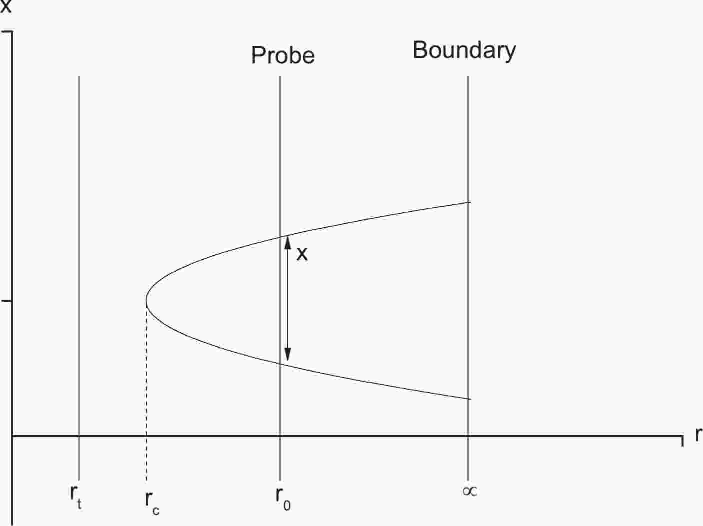
$ A(r_c) = A(r)|_{r = r_c} $ , where$ r = r_0 $ is an intermediate position in the bulk, which can yield a finite mass [6]. The configuration of the string world-sheet is shown in Fig. 1.
Figure 1. String configuration.
From (18) and (19), the inter-distance between
$ Q\bar{Q} $ is obtained as$ x = 2\int_{r_c}^{r_0}{\rm d}r\sqrt{\frac{A(r_c)B(r)}{A^2(r)-A(r)A(r_c)}} . $

(20) Substituting (15) and (19) into (12), the sum of the Coulomb potential and static energy is obtained as
$ V_{CP+E} = 2T_{\rm F}\int_{r_c}^{r_0}{\rm d}r\sqrt{\frac{A(r)B(r)}{A(r)-A(r_c)}}. $

(21) Next, we calculate the critical field. The DBI action is given by
$ S_{\rm DBI} = -T_{\rm D3}\int {\rm d}^4x\sqrt{-{\rm det}(G_{\mu\nu}+\mathcal{F}_{\mu\nu})} , $

(22) with
$ T_{D3} = \frac{1}{g_s(2\pi)^3\alpha^{\prime^2}}, \qquad \mathcal{F}_{\mu\nu} = 2\pi\alpha^\prime F_{\mu\nu}, $

(23) where
$T_{ D3}$ refers to the D3-brane tension.The induced metric reads
$\begin{aligned}[b] G_{00} =& -m(r)+n(r)p^2(r), \\ G_{11} =& G_{22} = r^2h(r),\\ G_{33} =& n(r),\\ G_{04} =& G_{40} = n(r)p(r). \end{aligned} $

(24) If the electric field is turned on along the x direction [8],
$ \begin{aligned}\\ {G_{\mu \nu }} + {{\cal F}_{\mu \nu }} = \left( {\begin{array}{*{20}{c}} { - m(r) + n(r){p^2}(r)}&{2\pi {\alpha ^\prime }E}&0&{n(r)p(r)}\\ { - 2\pi {\alpha ^\prime }E}&{{r^2}h(r)}&0&0\\ 0&0&{{r^2}h(r)}&0\\ {n(r)p(r)}&0&0&{n(r)} \end{array}} \right), \end{aligned}$ 
(25) yielding
$ {\rm det}(G_{\mu\nu}+\mathcal{F}_{\mu\nu}) = r^2h(r)n(r)\big[(2\pi\alpha^\prime)^2E^2-r^2h(r)m(r)\big]. $

(26) Inserting (26) into (22), and setting the probe D3-brane location at
$ r = r_0 $ , we get$ S_{\rm DBI} = -T_{ D3}r_0\sqrt{h_0n_0}\int {\rm d}^4x \sqrt{r_0^2h_0m_0-(2\pi\alpha^\prime)^2E^2} , $

(27) with
$ h_0 = h(r)|_{r = r_0} $ ,$ m_0 = m(r)|_{r = r_0} $ , etc.To avoid action (27) being ill-defined, we have
$ r_0^2h_0m_0-(2\pi\alpha^\prime)^2E^2\geq0, $

(28) which results in
$ E\leq\frac{r_0}{2\pi\alpha^\prime}\sqrt{h_0m_0} = T_{\rm F}r_0\sqrt{h_0m_0}. $

(29) As a result, the critical field is
$ E_c = T_{\rm F}r_0\sqrt{h_0m_0}, $

(30) and we can check that
$ E_c $ depends on T, c, and ω.Moreover, it is useful to give the mass of fundamental matter as
$ m = T_{\rm F}\int_{r_h}^{r_0} \sqrt{-{\rm det} g_{ab}} = T_{\rm F}(r_0-r_t), $

(31) with
$ m = m_0+\Delta m $ , where$ m_0 = T_{\rm F}r_0 $ is the mass in the system without T and ω, and$ \Delta m = -T_{\rm F}r_t $ depends on T and ω. Then, we can rewrite$ E_c $ as$ E_c = \frac{2\pi M^2}{\sqrt{\lambda}}\left(1-\frac{\Delta m}{m}\right)^2h_0\sqrt{\frac{f_0(1-\omega^2)}{1-f_0\omega^2}}, $

(32) where
$ E_c $ is well defined for T and ω with fixed$ r_0 $ .Now, we calculate the total potential. For convenience, we introduce the following dimensionless parameters:
$ \alpha\equiv\frac{E}{E_c}, \quad y\equiv\frac{r}{r_c},\quad a\equiv\frac{r_c}{r_0},\quad b\equiv\frac{r_t}{r_0}. $

(33) Then, the total potential becomes
$ \begin{aligned}[b] V_{\rm tot}(x) =& V_{CP+E}-Ex\\ =& 2ar_0T_{\rm F}\int_1^{1/a}{\rm d}y\sqrt{\frac{A(y)B(y)}{A(y)-A(y_c)}}\\& - 2ar_0T_{\rm F}\alpha r_0\sqrt{h_0m_0}\int_1^{1/a} {\rm d}y\sqrt{\frac{A(y_c)B(y)}{A^2(y)-A(y)A(y_c)}}, \end{aligned} $

(34) where
$ \begin{aligned}[b] A(y) =& (m(y)-n(y)p^2(y))(ar_0y)^2h(y),\\ B(y) =& (m(y)-n(y)p^2(y))h(y)/((ar_0y)^2f(y)),\\ A(y_c) =& (m(y_c)-n(y_c)p^2(y_c))(ar_0)^2h(y_c), \end{aligned} $

(35) with
$ \begin{aligned}[b] m(y) =& \frac{h(y)f(y)(ar_0y)^2(1-\omega^2)}{1-f(y)\omega^2},\\ n(y) =& h(y)(ar_0y)^2\gamma^2(1-f(y)\omega^2),\\ p(y) =& \frac{\omega(1-f(y))}{1-f(y)\omega^2},\\ m(y_c) =& \frac{h(y_c)f(y_c)(ar_0)^2(1-\omega^2)}{1-f(y_c)\omega^2},\\ n(y_c) =& h(y_c)(ar_0)^2\gamma^2(1-f(y_c)\omega^2),\\ p(y_c) =& \frac{\omega(1-f(y_c))}{1-f(y_c)\omega^2},\\ h(y) = & {\rm e}^{{c^2}/{(ar_0y)^2}}, \\ h(y_c) =& {\rm e}^{{c^2}/{(ar_0)^2}},\\ f(y) =& 1-\left(\frac{b}{ay}\right)^4,\\ f(y_c) = &1-\left(\frac{b}{a}\right)^4, \end{aligned}$

(36) and note that by setting
$ c = \omega = 0 $ in (34), the result of SYM [8] will be recovered.Before proceeding, we discuss the values of several parameters. First, for comparison purposes, we take
$ T_{\rm F} = 1 $ and$ b = 0.5/\sqrt{1-\omega^2} $ [8]. However, because the range$ 0\leq c/T\leq2.5 $ is most relevant for a comparison with QCD [55], we choose a value of c in that range.In Fig. 2, we plot
$ V_{\rm tot}(x) $ as a function of x for various cases, where the left panel is for$ c/T = 0, \omega = 0 $ , whereas the right is for$ c/T = 2.5, \omega = 0.2 \;{\rm GeV} $ (other cases with different values of$ c/T $ and ω result in similar plots). From both panels, we can see that for$ \alpha<1 $ (or$ E<E_c $ ), the potential barrier$ V_{\rm tot}(x) $ is present, and pair production can be described as a tunneling process. As E increases,$ V_{\rm tot}(x) $ decreases gradually and vanishes at$ \alpha = 1 $ (or$ E = E_c $ ). When$ \alpha>1 $ ($ E>E_c $ ), pair production is catastrophic, and the vacuum becomes catastrophically unstable. These findings are in accordance with [8].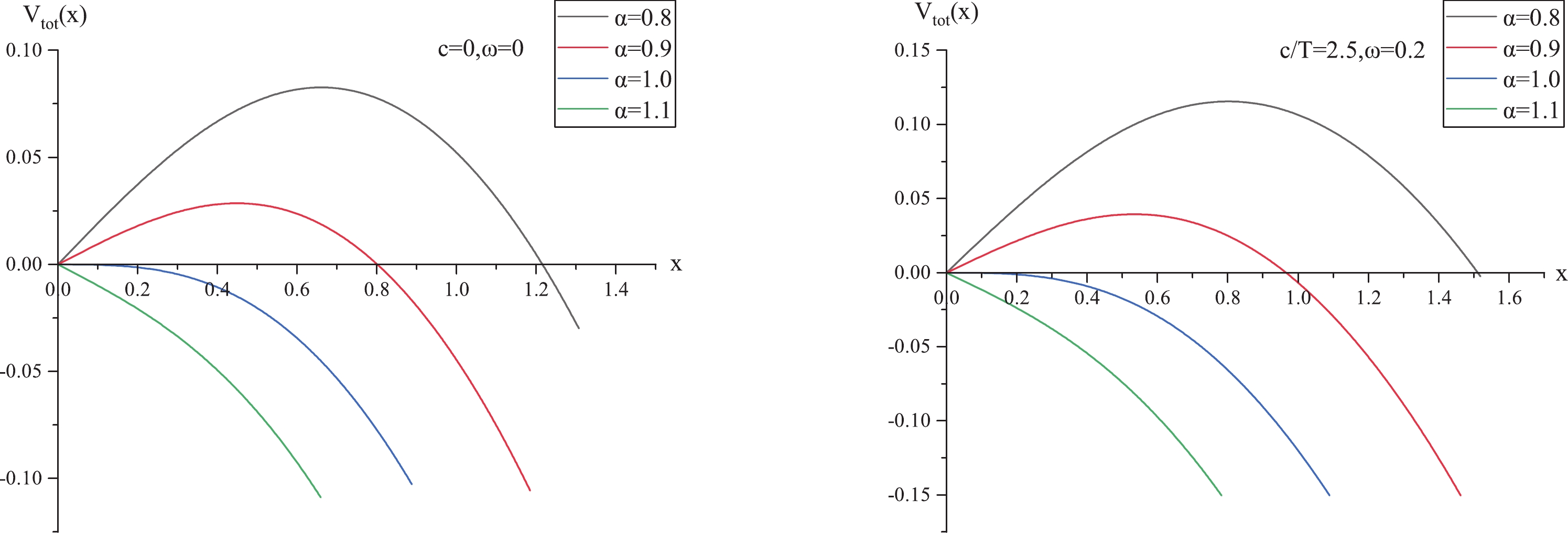
Figure 2. (color online)
$ V_{\rm tot}(x) $ versus x. (left)$ c/T = 0, \;\omega = 0 $ . (right)$ c/T = 2.5, \omega = 0.2 \ \;{\rm GeV} $ . In both panels, from top to bottom,$ \alpha = 0.8, \;0.9,\; 1, \;1.1 $ , respectively.To investigate how angular velocity affects the Schwinger effect, we plot
$ V_{\rm tot}(x) $ against x with fixed$ c/T $ for different values of ω in Fig. 3, where the left panel is for$ c/T = 0 $ , and the right panel is for$ c/T = 2.5 $ . In both panels, from top to bottom,$ \omega = 0, \;0.2,\; 0.6\;{\rm GeV} $ , respectively. At fixed$ c/T $ , the height and width of$ V_{\rm tot}(x) $ decrease with increasing ω. It is known that the higher or wider the potential barrier, the more forcefully the produced pairs escape to infinity. Therefore, we can draw the conclusion that the inclusion of angular velocity decreases the potential barrier, thus enhancing the Schwinger effect, that is, producing$ Q\bar{Q} $ pairs would be easier in the presence of angular velocity. Furthermore, by comparing the left and right panels, we find that c has the opposite effect, that is, increasing c increases$ V_{\rm tot}(x) $ , thus reducing the Schwinger effect, consistent with the findings of [14].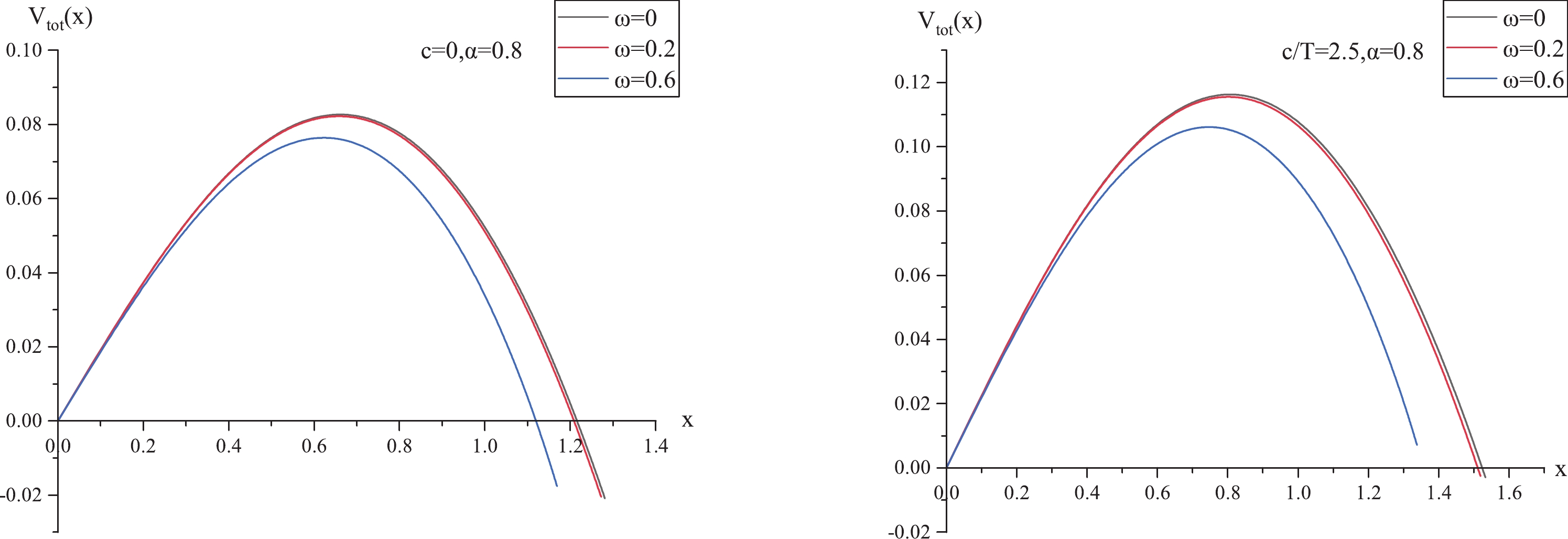
Figure 3. (color online)
$ V_{\rm tot}(x) $ versus x with$ \alpha = 0.8 $ and fixed$ c/T $ for different values of ω. In both plots, from top to bottom,$ \omega = 0,\; 0.2,\; 0.6 \ \;{\rm GeV} $ , respectively.Moreover, to observe how angular velocity modifies the critical electric field, we plot
$ E_c/E_{c0} $ versus ω in Fig. 4, where$ E_{c0} $ represents the critical electric field of SYM. We find that$ E_c/E_{c0} $ decreases as ω increases, implying that the inclusion of angular velocity decreases$ E_c $ , thus making the tunneling process easier, which is in agreement with the potential analysis. Meanwhile, c has the opposite effect. In addition,$ E_c/E_{c0} $ can be smaller or larger than 1, which means that the model considered in this study could provide a wider range for the Schwinger effect in comparison to SYM.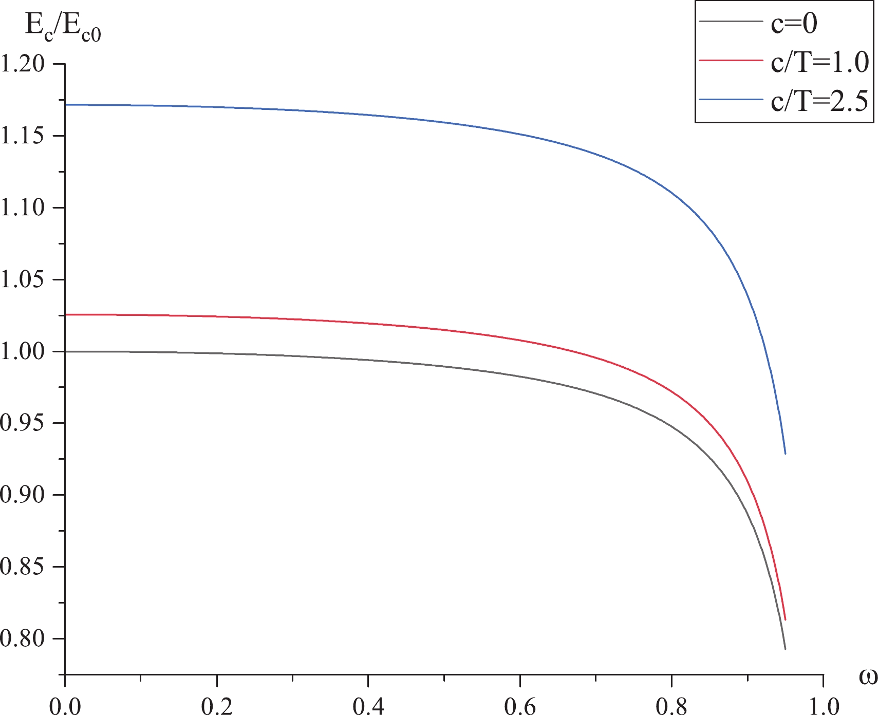
Figure 4. (color online)
$ E_c/E_{c0} $ versus ω. In both plots, from top to bottom,$ c/T = 2.5, \;1, \;0 $ , respectively. -
In this paper, we investigate the effect of angular velocity on the Schwinger effect using potential analysis in a deformed AdS black-hole background. We calculate the total potential of a
$ Q\bar{Q} $ pair in an external electric field and determine the critical electric field from DBI action. It is found that the inclusion of angular velocity enhances the Schwinger effect, in contrast with the effect of the confining scale c. Moreover, with several chosen values of ω and$ c/T $ ,$ E_c $ can be smaller or larger than its counterpart in SYM, indicating that the model considered here could theoretically provide a wider range for the Schwinger effect in comparison to SYM.Interestingly, the holographic Schwinger effect has previously been discussed in a moving medium [13], and the results showed that the presence of velocity increases the Schwinger effect. Taken together, we may summarize that translation and rotation have the same effect on the Schwinger effect. Furthermore, the production of
$ Q\bar{Q} $ pairs would be easier in a moving or rotating medium. One likely explanation for this is that in moving or rotating backgrounds, virtual pairs may not only gain energy from the external electric field but also from the kinetic energy associated with translation and rotation. However, the exact mechanism is not yet clear and requires further investigation.Finally, it is interesting to note that rotating QGP may also be described by means of a five-dimensional Kerr-AdS black hole [56], and one may also study the Schwinger effect in that rotating frame. We hope to report our progress on this in the near future.
Holographic Schwinger effect in a rotating strongly coupled medium
- Received Date: 2022-04-06
- Available Online: 2022-10-15
Abstract: We perform a potential analysis on the holographic Schwinger effect in a rotating deformed AdS black-hole background. We calculate the total potential of a quark-antiquark (


 DownLoad: