


 Abstract
 HTML
HTML Reference
 Related
 PDF
PDF


-
As high energy physics continues to develop, the sensitivity of detectors has been improving and a large number of data samples are accumulated, which makes experimental measurements increasingly precise. Therefore, the predictions from the theoretical side must be sufficiently precise to match the measurements, which demands the calculation of higher order perturbative corrections. Fortunately, the technology of Feynman amplitude calculations has also been significantly improved in recent years. Today, automatic one-loop calculations are already available, provided by many different packages (see e.g., [1–5]). Automatic multi-loop calculations are still under process, but significant progress has already been achieved (see e.g., [6–10]).
Meanwhile, multi-particle processes are becoming increasingly important in this procedure. For example, it is well known that in future
$ e^{+}e^{-} $ colliders such as the International Linear Collider (ILC) and the Compact Linear Collider (CLIC), the pair production of the top quark$ e^{+}e^{-}\rightarrow t\overline{t} $ will be very important [11–15]. In this process, the top pair will decay, resulting in a series of subprocesses with six final states.On one hand, owing to the high luminosity, such subprocesses can be directly measured and studied. On the other hand, their contributions are comparable with certain higher order corrections; thus, they should not be neglected even in perturbative calculations.
The calculation of such processes is straightforward but cumbersome, even at the tree level. This is because the number of Feynman diagrams increases very rapidly as external particles increase such that the expression of total scattering amplitude becomes very complicated. Despite some special cases, such calculations can only be performed numerically.
This becomes even more complicated if fermions exist in the external particles. The scattering amplitude of a process with external fermions can be crudely expressed as
$ {\cal{M}} \sim \sum\limits_{i} F_{i_1}F_{i_2}\cdots F_{i_n}. $

(1) We have used
$ \sim $ in the expression since the coefficients have been dropped. Here,$ F_k $ denotes a fermion line, which contains a string of Dirac γ-matrices and two spinors, i.e.,$ F_k = \overline{U}_1 \widehat{V}_1\cdots \widehat{V}_m U_2. $

(2) Here,
$ U_{1,2} $ are the two spinors, and$ V_{1,2,\cdots,m} $ are several vectors, which can be external momenta, polarization vectors, and their combinations. We use a hat ($ \widehat{\ } $ ) over a vector to denote its contraction with the Dirac matrices, i.e.,$ \widehat{V}\equiv g_{\mu \nu}V^\mu \gamma^{\nu}, $

(3) with
$ g_{\mu \nu} $ =diag$ \{1,-1,-1,-1\} $ and$ \gamma^{\mu} $ =$ (\gamma^0,\gamma^1,\gamma^2,\gamma^3) $ .Since physical results are described by the square of the amplitude, the conventional method to evaluate Eq. (1) is squaring it with its Hermitian conjugation and summing over the fermion polarizations using Dirac equation. Thus, the square of the amplitude can be expressed as
$ |{\cal{M}}|^2 \sim \sum\limits_{j} \mathrm{Tr}S^{(n_{j_1})}_{j_1} \mathrm{Tr}S_{j_2}^{(n_{j_2})} \cdots \mathrm{Tr}S_{j_l}^{(n_{j_l})}, $

(4) where
$ S_i^{(n_{i})} $ denotes a string with$ n_i $ Dirac matrices. Each of them is obtained from at least two fermion lines such that it is apparent that numerous matrix multiplications will be present in the calculation, which is time-consuming. Furthermore, in multi-particle processes, the number of total terms in Eq. (1) increases very rapidly, which results in a significantly large number of terms after the squaring. Therefore, this conventional method is not applicable in multi-particle processes.An alternative method is to calculate the amplitude directly before squaring it. A fermion line
$ F_k $ can be converted into a trace by moving the second spinor to the front, i.e.,$ F_k=\mathrm{Tr}(U_2\overline{U}_1 \widehat{V}_1\cdots \widehat{V}_m). $

(5) With specific polarizations,
$ U_2\overline{U}_1 $ is only a$ 4\times4 $ matrix; therefore, it can be expanded over γ-matrices. Many different forms of the expansion result in different approaches (see e.g., [16–20]).Another popular approach is the helicity amplitude method [21–27]. For a certain helicity configuration of external particles, the amplitude can be simplified since many of the terms do not contribute. Meanwhile, amplitudes with different helicity configurations do not interfere with each other; hence, the square of the total amplitude becomes straightforward.
In recent years, a new approach, based on on-shell recursion relations, has become popular in the calculation of the scattering amplitude. In this approach, the amplitude of multi-particle processes is constructed with blocks from on-shell amplitudes of fewer legs, which is much simpler than the original one. The most famous on-shell recursion relations are the "BCFW recursion relations" proposed by Britto, Cachazo, Feng, and Witten in the calculation of gluon scattering [28, 29]. The recursion relations are derived using complex deformations of the external momenta and calculating the residue of the deformed amplitude in the complex plane. Combined with the spinor helicity formalism, this approach has demonstrated significant advantages in the scattering of massless particles. This approach cannot be directly applied to processes with massive particles since the momenta of massive particles cannot be expressed as a direct product of two spinors. Many efforts have been conducted on this [30–39].
In this paper, we introduce a new numerical algorithm for calculating fermion lines at the tree level. By avoiding most time-consuming matrix multiplications, this new approach can reduce the time used in the calculation of amplitudes and hence increases the efficiency of phase space integration and event generation, partiuclarly in the processes with many fermion lines.
The remainder of this paper is organized as follows: In Section II, we introduce our new algorithm, including the calculation of γ-matrix strings, the calculation of fermion lines, and the calculation of the amplitudes with fermion lines. In Section III, a comparison with other programs is presented to demonstrate the advantage of the new algorithm that is implemented in our FDC package [40]. The summary is given in the final section.
-
First, our approach is limited to the tree level; hence, the dimension of space-time is always 4. Additionally, for the γ-matrices, the Dirac (standard) representation is used, i.e.,
$ \begin{array}{l} \gamma^0 = \left( \begin{array}{l} 1 \quad 0 \\ 0 \quad -1 \end{array} \right), \gamma^i = \left( \begin{array}{l} 0 \quad \sigma^i \\ -\sigma^i \quad 0 \end{array} \right), \gamma^5 = \left( \begin{array}{l} 0 \quad 1 \\ 1 \quad 0 \end{array} \right),\quad \end{array} $

(6) with
$ i=1,2,3 $ .$ \sigma_i $ are the Pauli matrices:$ \begin{array}{l} \sigma^1 = \left( \begin{array}{l} 0 \quad 1 \\ 1 \quad 0 \end{array} \right), \sigma^2 = \left( \begin{array}{l} 0 \quad -i \\ i \quad 0 \end{array} \right), \sigma^3 = \left( \begin{array}{l} 1 \quad 0 \\ 0 \quad -1 \end{array} \right). \quad \end{array} $

(7) The contraction of a four-dimensional vector
$ p^\mu=(p^0,\vec{p}) $ with the γ-matrices takes the form of$ \widehat{p}=p^0\gamma^0-\vec{p}\cdot \vec{\gamma}= \left( \begin{array}{l} p^0 \quad -\vec{p}\cdot\vec{\sigma} \\ \vec{p}\cdot\vec{\sigma} \quad -p^0 \end{array} \right). $

(8) The string with
$ n ~ \gamma $ -matrices is defined as$ S^{(n)}(p_n,p_{n-1},\cdots,p_1)=\widehat{p}_n\widehat{p}_{n-1}\cdots\widehat{p}_1. $

(9) The order of superscripts in the vectors has been reversed for convenience.
The Dirac spinors for a fermion and anti-fermion are defined as
$ \begin{aligned}[b] u(k,s)\equiv& U(+,k,s)=\dfrac{\widehat{k}+m}{\sqrt{k^0+m}}u_0 (+,s), \\ v(k,s)\equiv& U(-,k,s)=\dfrac{-\widehat{k}+m}{\sqrt{k^0+m}}u_0 (-,s), \end{aligned} $

(10) with
$ u_0(+,s)\equiv\left(\begin{array}{l} \chi_s \\ 0 \end{array}\right), \quad u_0(-,s)\equiv \left(\begin{array}{l} 0 \\ \chi_s \end{array}\right), $

(11) and
$ \chi_1=\left(\begin{array}{l} 1 \\ 0 \end{array}\right), \quad \chi_2=\left(\begin{array}{l} 0 \\ 1 \end{array}\right). $

(12) Here, the symbols
$ \pm $ in U and$ u_0 $ are used to distinguish the fermion and anti-fermion, and s is the polarization of the particle. -
In this subsection, we introduce the recursive calculation of
$ S^{(n)} $ , the string with$ n ~ \gamma $ -matrices. In the calculation of the amplitude,$ \gamma^5 $ might be present among other γ-matrices. Owing to its anti-commutativity with all the γ-matrices, all the$ \gamma^5 $ matrices can be moved outside of$ S^{(n)} $ by adding a possible factor$ -1 $ . Meanwhile, we assume that all the Lorentz indices have been summed over in the string; therefore, all the γ-matrices in$ S^{(n)} $ are now contracted with certain vectors, i.e., it assumes exactly the form of Eq. (9). -
We will show later that the cases of
$ n=0, 1 $ are not required. Here, we simply skip them and begin from$ n=2 $ . According to Eq. (8),$ S^{(2)} $ can be rewritten as$ \begin{aligned}[b]& S^{(2)}(p_2,p_1) \\=& \left( \begin{array}{rrr} p_2^0 & -\vec{p}_2\cdot\vec{\sigma} \\ \vec{p}_2\cdot\vec{\sigma} & -p_2^0 \end{array} \right) \left( \begin{array}{rrr} p_1^0 & -\vec{p}_1\cdot\vec{\sigma} \\ \vec{p}_1\cdot\vec{\sigma} & -p_1^0 \end{array} \right) \\ =&\left( \begin{array}{rrr} p_2^0 p_1^0-(\vec{p}_2\cdot\vec{\sigma})( \vec{p}_1\cdot\vec{\sigma})& p_1^0 (\vec{p}_2\cdot\vec{\sigma})-p_2^0(\vec{p}_1\cdot\vec{\sigma}) \\ p_1^0 (\vec{p}_2\cdot\vec{\sigma})-p_2^0(\vec{p}_1\cdot\vec{\sigma})& p_2^0 p_1^0-(\vec{p}_2\cdot\vec{\sigma} )(\vec{p}_1\cdot\vec{\sigma}) \end{array} \right). \end{aligned} $

(13) Using the identity of Pauli matrices
$ \sigma^i\sigma^j= {\rm i}\varepsilon^{ijk}\sigma^k+\delta^{ij}, $

(14) we easily determine
$ \begin{aligned}[b] (\vec{p}_2\cdot\vec{\sigma})(\vec{p}_1\cdot\vec{\sigma})&=p_2^i\sigma^ip_1^j\sigma^j\\ &=p_2^ip_1^j({\rm i}\varepsilon^{ijk}\sigma^k+\delta^{ij})\\ &={\rm i}\varepsilon^{ijk}p_2^ip_1^j\sigma^k+\vec{p}_2\cdot\vec{p}_1. \end{aligned} $

(15) Hence,
$ S^{(2)}(p_2,p_1) =\left( \begin{array}{rrr} p_2\cdot p_1-{\rm i}\varepsilon^{ijk}p_2^ip_1^j\sigma^k& (p_1^0 \vec{p}_2-p_2^0\vec{p}_1)\cdot\vec{\sigma} \\ (p_1^0 \vec{p}_2-p_2^0\vec{p}_1)\cdot\vec{\sigma} & p_2\cdot p_1-{\rm i}\varepsilon^{ijk}p_2^ip_1^j\sigma^k \end{array} \right). $

(16) On the other hand, by introducing two new vectors
$ p_a $ and$ p_b $ as$ \begin{aligned}[b] p_a^{(2),\mu}(p_2,p_1)&\equiv(p_2\cdot p_1, -p_2^0\vec{p}_1+p_1^0\vec{p}_2),\\ p_b^{(2),\mu}(p_2,p_1)&\equiv(0, \varepsilon^{ijk}p_2^ip_1^j), \end{aligned} $

(17) $ S^{(2)} $ in Eq. (16) can be further expressed as$ S^{(2)}(p_2,p_1)=\widehat{p}_{a,\{2,1\}}^{(2)}\gamma^0- {\rm i} \gamma^5\widehat{p}_{b,\{2,1\}}^{(2)}\gamma^0. $

(18) Here, the superscript
$ (2) $ in$ p_a $ and$ p_b $ denotes that the vector contains two arguments, which is the same as$ S^{(n)} $ . Additionally, we have used the abbreviation to compact the expression$ {p}_{a(b),\{i_n,i_{n-1},\cdots,i_1\}}^{(n)}\equiv{p}_{a(b)}^{(n)}(p_{i_n},p_{i_{n-1}},\cdots,p_{i_1}). $

(19) -
The calculation of
$ S^{(3)} $ is straightforward using Eq. (18)$ \begin{aligned}[b] S^{(3)}(p_3,p_2,p_1) =&\widehat{p}_3S^{(2)}(p_2,p_1) \\ =&\widehat{p}_3\left(\widehat{p}_{a,\{2,1\}}^{(2)}\gamma^0- {\rm i} \gamma^5\widehat{p}_{b,\{2,1\}}^{(2)}\gamma^0\right) \\ =&S^{(2)}\left(p_3,{p}_{a,\{2,1\}}^{(2)}\right)\gamma^0+ {\rm i} \gamma^5S^{(2)}\left(p_3,{p}_{b,\{2,1\}}^{(2)}\right)\gamma^0. \end{aligned} $

(20) The two
$ S^{(2)} $ on the r.h.s. of Eq. (20) can be obtained by using Eq. (18) again:$ \begin{aligned}[b]S^{(2)}\left(p_3,{p}_{a(b),\{2,1\}}^{(2)}\right) =&\widehat{p}^{(2)}_{a}\left(p_3,{p}_{a(b),\{2,1\}}^{(2)}\right)\gamma^0 \\ &-{\rm i}\gamma^5\widehat{p}^{(2)}_{b}\left(p_3,{p}_{a(b),\{2,1\}}^{(2)}\right)\gamma^0. \end{aligned} $

(21) Inserting them into Eq. (20), we obtain
$ \begin{aligned}[b] S^{(3)}(p_3,p_2,p_1) =&\left[\widehat{p}^{(2)}_{a}\left(p_3,{p}_{a,\{2,1\}}^{(2)}\right)+\widehat{p}^{(2)}_{b}\left(p_3,{p}_{b,\{2,1\}}^{(2)}\right)\right] \\ & -{\rm i}\gamma^5\left[\widehat{p}^{(2)}_{b}\left(p_3,{p}_{a,\{2,1\}}^{(2)}\right)-\widehat{p}^{(2)}_{a}\left(p_3,{p}_{b,\{2,1\}}^{(2)}\right)\right]. \end{aligned} $

(22) By introducing two new vectors as
$ \begin{aligned}[b] p^{(3)}_a(p_3,p_2,p_1)\equiv&{p}^{(2)}_{a}\left(p_3,{p}_{a,\{2,1\}}^{(2)}\right)+{p}^{(2)}_{b}\left(p_3,{p}_{b,\{2,1\}}^{(2)}\right), \\ p^{(3)}_b(p_3,p_2,p_1)\equiv&{p}^{(2)}_{b}\left(p_3,{p}_{a,\{2,1\}}^{(2)}\right)-{p}^{(2)}_{a}\left(p_3,{p}_{b,\{2,1\}}^{(2)}\right), \\ \end{aligned} $

(23) $ S^{(3)} $ can be expressed as$ S^{(3)}(p_3,p_2,p_1)=\widehat{p}^{(3)}_{a,\{3,2,1\}}-{\rm i}\gamma^5\widehat{p}^{(3)}_{b,\{3,2,1\}}. $

(24) -
The calculation for the case of
$ n=4 $ is similar to that of$ n=3 $ . Using Eq. (24),$ S^{(4)} $ is expressed by two other$ S^{(2)} $ as$ \begin{aligned}[b] S^{(4)}(p_4,p_3,p_2,p_1) =&\widehat{p_4}\left[\widehat{p}^{(3)}_{a,\{3,2,1\}}-{\rm i}\gamma^5\widehat{p}^{(3)}_{b,\{3,2,1\}}\right] \\ =&S^{(2)}\left(p_4,{p}^{(3)}_{a,\{3,2,1\}}\right)+{\rm i}\gamma^5S^{(2)}\left(p_4,{p}^{(3)}_{b,\{3,2,1\}}\right) . \end{aligned} $

(25) These
$ S^{(2)} $ are then obtained using Eq. (18) as$ \begin{aligned}[b] S^{(2)}\left(p_4,{p}_{a(b),\{3,2,1\}}^{(3)}\right) =&\widehat{p}^{(2)}_{a}\left(p_4,{p}_{a(b),\{3,2,1\}}^{(3)}\right)\gamma^0 \\ &-{\rm i}\gamma^5\widehat{p}^{(2)}_{b}\left(p_4,{p}_{a(b),\{3,2,1\}}^{(3)}\right)\gamma^0 . \end{aligned} $

(26) Inserting them into Eq. (25) yields
$ \begin{aligned}[b] S^{(4)}(p_4,p_3,p_2,p_1) =&\left[\widehat{p}^{(2)}_{a}\left(p_4,{p}_{a,\{3,2,1\}}^{(3)}\right)+\widehat{p}^{(2)}_{b}\left(p_4,{p}_{b,\{3,2,1\}}^{(3)}\right)\right]\gamma^0 \\ &-{\rm i}\gamma^5\Big[\widehat{p}^{(2)}_{b}\left(p_4,{p}_{a,\{3,2,1\}}^{(3)}\right)\\&-\widehat{p}^{(2)}_{a}\left(p_4,{p}_{b,\{3,2,1\}}^{(3)}\right)\Big]\gamma^0 \\ =&\widehat{p}_{a,\{4,3,2,1\}}^{(4)}\gamma^0-{\rm i}\gamma^5\widehat{p}_{b,\{4,3,2,1\}}^{(4)}\gamma^0, \end{aligned} $

(27) where the two new vectors are defined as
$ \begin{aligned}[b] p^{(4)}_a(p_4,p_3,p_2,p_1)\equiv&{p}^{(2)}_{a}\left(p_4,{p}_{a,\{3,2,1\}}^{(3)}\right)+{p}^{(2)}_{b}\left(p_4,{p}_{b,\{3,2,1\}}^{(3)}\right), \\ p^{(4)}_b(p_4,p_3,p_2,p_1)\equiv&{p}^{(2)}_{b}\left(p_4,{p}_{a,\{3,2,1\}}^{(3)}\right)-{p}^{(2)}_{a}\left(p_4,{p}_{b,\{3,2,1\}}^{(3)}\right). \\ \end{aligned} $

(28) We can observe that
$ S^{(4)} $ in Eq. (27) has the same form as$ S^{(2)} $ ; therefore,$ S^{(5)} $ will have the same form as$ S^{(3)} $ . Generalizing this to even larger n, we arrive at the general formula of$ S^{(n)} $ ($ n\ge2 $ ):$ \begin{aligned}[b]& S^{(n)}(p_n,p_{n-1},\cdots,p_1)\\=& \begin{cases} \widehat{p}_{a,\{n,n-1,\cdots,1\}}^{(n)}\gamma^0-{\rm i}\gamma^5\widehat{p}_{b,\{n,n-1,\cdots,1\}}^{(n)}\gamma^0 &\qquad \text{for even}~~ n \\ \widehat{p}_{a,\{n,n-1,\cdots,1\}}^{(n)}-{\rm i}\gamma^5\widehat{p}_{b,\{n,n-1,\cdots,1\}}^{(n)} &\qquad \text{for odd}~~ n \end{cases} \end{aligned} $

(29) which can be further rewritten as
$ \begin{aligned}[b] &S^{(n)}(p_n,p_{n-1},\cdots,p_1) \\ =&\left( \widehat{p}_{a,\{n,n-1,\cdots,1\}}^{(n)}-{\rm i}\gamma^5\widehat{p}_{b,\{n,n-1,\cdots,1\}}^{(n)}\right)(\gamma^0)^{n+1}. \end{aligned} $

(30) Meanwhile, from Eqs. (23) and (28), we observe that
$ p_a^{(n)} $ and$ p_b^{(n)} $ ($ n\ge3 $ ) always have the same form whether n is odd or even. It can be obtained recursively as$ \begin{aligned}[b] p^{(n)}_a(p_n,p_{n-1},\cdots,p_1) \equiv&{p}^{(2)}_{a}\left(p_n,{p}_{a,\{n-1,\cdots,1\}}^{(n-1)}\right)\\&+{p}^{(2)}_{b}\left(p_n,{p}_{b,\{n-1,\cdots,1\}}^{(n-1)}\right),\\ p^{(n)}_b(p_n,p_{n-1},\cdots,p_1) \equiv&{p}^{(2)}_{b}\left(p_n,{p}_{a,\{n-1,\cdots,1\}}^{(n-1)}\right)\\&-{p}^{(2)}_{a}\left(p_n,{p}_{b,\{n-1,\cdots,1\}}^{(n-1)}\right), \end{aligned} $

(31) while
$ p_{a(b)}^{(2)} $ is defined in Eq. (17).Let us further investigate the structure of
$ S^{(n)} $ . Eq. (30) can be considered as another definition of$ S^{(n)} $ , in which the arguments are no longer$ p_i $ , but$ p_a $ and$ p_b $ . For a fixed queue of$ p_i $ ,$ p_a $ and$ p_b $ can be obtained using Eq. (31); thus, the corresponding$ S^{(n)} $ is expressed as$ S^{(n)}(p_a,p_b)=\left( \widehat{p}_{a}-{\rm i}\gamma^5\widehat{p}_{b}\right)(\gamma^0)^{n+1}\equiv \widetilde{S}^{(n)}(p_a,p_b)(\gamma^0)^{n+1}. $

(32) A tilde is used over
$ S^{(n)} $ to denote the part without$ \gamma^0 $ . Using Eqs. (6) and (8), we easily observe that$ \widetilde{S}^{(n)} $ can be expressed using four blocks as$ \widetilde{S}^{(n)}(p_a,p_b)= \left( \begin{array}{l} A^{(++)} \quad A^{(+-)} \\ A^{(-+)} \quad A^{(--)} \end{array} \right), $

(33) with
$ \begin{aligned}[b] A^{(++)}&=-A^{(--)}=p_a^0-{\rm i}\vec{p}_b\cdot \vec{\sigma} , \\ A^{(+-)}&=-A^{(-+)}={\rm i}p_b^0-\vec{p}_a\cdot \vec{\sigma} . \end{aligned} $

(34) Only two of them are independent.
Also, from Eq. (32) it is straightforward to derive the product of
$ \gamma^5 $ and$ S^{(n)} $ :$ \begin{aligned}[b] \gamma^5S^{(n)}(p_a,p_b)=& \left(\gamma^5\widehat{p}_{a}-{\rm i}\widehat{p}_{b}\right)(\gamma^0)^{n+1} \\ =&(-{\rm i})\left(\widehat{p}_{b}+{\rm i}\gamma^5\widehat{p}_{a}\right)(\gamma^0)^{n+1}\\ =&-{\rm i}S^{(n)}(p_b,-p_a). \end{aligned} $

(35) -
In this subsection, we introduce the calculation of the fermion lines using the string
$ S^{(n)} $ we have obtained above. A fermion line with two external fermions can frequently be expressed as$ \begin{aligned}[b] &F(z_1, k_1, s_1;z_2, k_2, s_2; n)\\ =&\overline{U}(z_1,k_1,s_1)S^{(n)}(p_n,p_{n-1},\cdots,p_1)U(z_2,k_2,s_2). \end{aligned}$

(36) In this expression
$ {U}(z,k,s) $ , which is defined in Eq. (10), is used as the spinor of the fermion and anti-fermion simultaneously. Here, z can be$ + $ or$ - $ , which denote the fermion or anti-fermion, respectively. k and s are the momentum and polarization of the particle, respectively. Note that for a specific process, all the$ z_i $ values are fixed according to external particles. n in the arguments of F denotes a string of$ n ~ \gamma $ -matrices, but we have removed the detailed list of vectors for convenience.In the calculation of amplitude,
$ \gamma^5 $ might be present in a fermion line. However, owing to its anti-commutativity with all four γ-matrices, it can always be moved in front of$ S^{(n)} $ . Furthermore, according to Eq. (35),$ \gamma^5S^{(n)} $ can be obtained by a substitution in the arguments of$ S^{(n)} $ . Hence, there is no particular need to discuss calculating fermion lines with$ \gamma^5 $ . -
First, we introduce a trick in the spinors. As shown in Eq. (10), the relationship between
$ U(z, k, s) $ and$ u_0(z,s) $ can be expressed as$ U(z,k,s)=\dfrac{z\widehat{k}+m}{\sqrt{k^0+m}}u_0 (z,s). $

(37) If we introduce a new vector, which is defined as
$ k^{\prime\mu}\equiv\dfrac{1}{\sqrt{k^0+m}}({k^0+m},\vec{k}), $

(38) it is easy to prove
$\begin{aligned}[b]& U(z,k,s)=z\widehat{k}^\prime u_0 (z,s), \\& \overline{U}(z,k,s)=z \overline{u}_0 (z,s)\widehat{k}^\prime. \end{aligned} $

(39) This trick is very useful if massive fermions are present since it prevents the term
$ z\widehat{k}+m $ from being separated. In a process with n massive fermions, this trick can reduce the number of total terms by a factor of$ 1/2^n $ .Meanwhile, we can observe that in the Dirac presentation,
$ u_0 $ , defined in Eq. (11), is an eigenstates of$ \gamma^0 $ with the eigenvalue z, i.e.,$ \gamma^0 u_0(z,s)=z u_0(z, s), \quad u_0(z,s)^\dagger \gamma^0 =z u_0(z, s)^\dagger. $

(40) -
Now we return to the calculation of fermion lines. Here, we still assume that all the Lorentz indices have been summed over in the string of γ-matrices; hence, no Lorentz indices remain.
Using Eqs. (39) and (40), we easily observe that
$ \begin{aligned}[b]&F(z_1, k_1, s_1;z_2, k_2, s_2;n) \\ =&\overline{U}(z_1,k_1,s_1)S^{(n)}(p_n,p_{n-1},\cdots,p_1)U(z_2,k_2,s_2) \\ =&z_1z_2\overline{u}_0(z_1,s_1)\widehat{k}_1^\prime S^{(n)}(p_n,p_{n-1},\cdots,p_1) \widehat{k}_2^\prime u_0(z_2,s_2) \\ =&z_1z_2\overline{u}_0(z_1,s_1)S^{(n+2)}(k_1^\prime, p_n,p_{n-1},\cdots,p_1, k_2^\prime)u_0(z_2,s_2). \end{aligned} $

(41) The momenta are separated from the spinors and merged to the string of γ-matrices
$ S^{(n+2)} $ . This procedure can be conducted for all the fermion lines, which indicates all the$ S^{(n)} $ we must calculate contain at least two γ-matrices. This is why in Sec. II.B only the cases of$ n\ge2 $ are considered.The r.h.s. of Eq. (41) can be further evaluated using Eqs. (32) and (33) as
$ \begin{aligned}[b]&F(z_1, k_1, s_1;z_2, k_2, s_2;n) \\ =&z_1z_2{u}_0(z_1,s_1)^\dagger\gamma^0\widetilde{S}^{(n+2)}(\gamma^0)^{n+3}u_0(z_2,s_2) \\ =&z_1^2z_2^{n+4}{u}_0(z_1,s_1)^\dagger \left( \begin{array}{l}A^{(++)} \quad A^{(+-)} \\ A^{(-+)} \quad A^{(--)}\end{array} \right)u_0(z_2,s_2) \\ =&z_2^{n}\chi_{s_1}^\dagger A^{(z_1z_2)}\chi_{s_2} = z_2^n A^{(z_1z_2)}_{s_1s_2}, \end{aligned} $

(42) where Eq. (40) and
$ z_1^2=z_2^2=1 $ have been used.As mentioned earlier,
$ z_{1,2} $ is fixed for a specific process; hence, only one of the four blocks in$ \widetilde{S}^{(n+2)} $ is required. Since$ \widetilde{S}^{(n+2)} $ is totally decided by$ p_a $ and$ p_b $ , the calculation of the fermion line is now converted into the calculation of$ p_a $ and$ p_b $ , which can be performed recursively without any matrix multiplications.Furthermore, four elements of the block
$ A^{(z_1z_2)} $ corresponds to the four different configurations of$ \{s_1,s_2\} $ , respectively. This means that the results for all possible polarization configurations can be obtained via a single calculation, which can significantly increase the efficiency of calculation. -
Thus far, we have assumed that all the Lorentz indices are summed over in fermion lines, but that is insufficient for the calculation of the amplitude. In this section, we introduce the calculation of fermion lines with one Lorentz index, which have the form
$ \begin{aligned}[b] &F^\mu(z_1, k_1, s_1;z_2, k_2, s_2; n_1,n_2) \\ =&\overline{U}(z_1,k_1,s_1)S^{(n_1)}(p_{n_1},\cdots,p_1)\gamma^\mu \\ & \times S^{(n_2)}(q_{n_2},\cdots,q_1)U(z_2,k_2,s_2). \end{aligned} $

(43) It is a Lorentz vector with four components. To calculate these four components, we introduce four auxiliary vectors as follows
$ \begin{aligned}[b]& r^\mu_0=\{1 , 0 , 0 , 0\}, \quad r^\mu_1=\{0 , -1 , 0 , 0\}, \\ & r^\mu_2=\{0 , 0 , -1 , 0\}, \quad r^\mu_3=\{0 , 0 , 0 , -1\}. \end{aligned} $

(44) It is clear that
$ \gamma^0=\widehat{r}_0, \quad \gamma^i=\widehat{r}_i . $

(45) Hence,
$ \begin{aligned}[b]& F^0(z_1, k_1, s_1;z_2, k_2, s_2; n_1,n_2) \\ =&\overline{U}(z_1,k_1,s_1)S^{(n_1)}(p_{n_1},\cdots,p_1)\gamma^0S^{(n_2)}(q_{n_2},\cdots,q_1)U(z_2,k_2,s_2) \\ =&\overline{U}(z_1,k_1,s_1)S^{(n_1)}(p_{n_1},\cdots,p_1)\widehat{r}_0S^{(n_2)}(q_{n_2},\cdots,q_1)U(z_2,k_2,s_2) \\ =&\overline{U}(z_1,k_1,s_1)S^{(n_1+n_2+1)}(p_{n_1},\cdots,p_1,{r}_0,q_{n_2},\cdots,q_1)U(z_2,k_2,s_2). \end{aligned} $

This is exactly the result of a fermion line without any Lorentz indices. Similarly, the other three components are obtained as
$\begin{aligned}[b]& F^i(z_1, k_1, s_1;z_2, k_2, s_2; n_1,n_2) \\=&\overline{U}(z_1,k_1,s_1)S^{(n_1+n_2+1)}(p_{n_1},\cdots,p_1,{r}_i,q_{n_2},\cdots,q_1)U(z_2,k_2,s_2) .\end{aligned} $

(46) -
The scattering amplitude of a process with n fermion lines often has the form
$ {\cal{M}}\sim \sum\limits_i F_{i_1}F_{i_2}\cdots F_{i_n}, $

(47) where the coefficients have been dropped. It is natural to assume that the summation over Lorentz indices has already been performed inside each fermion line. Thereafter, we can separate the fermion lines into three types: 1) with no Lorentz indices; 2) with one Lorentz index; 3) with two or more Lorentz indices. To calculate the amplitude, we must calculate all these three types of fermion lines.
We have already presented a detailed introduction on calculating fermion lines without indices; hence, we need not to discuss them here. Meanwhile, as mentioned earlier, fermion lines with one index are Lorentz vectors, whose components can be obtained by introducing four auxiliary vectors. It should be emphasized that when obtained, these vectors can also be contracted into other fermion lines.
Thus far, we have not mentioned how to address fermions lines with two or more indices. Of course, they can be considered as Lorentz tensors, and all of their components can be obtained with the four auxiliary vectors, similar to those with one index. However, a better method is available.
First, we would like to indicate that, at tree level, if there are n pairs of Lorentz index contractions among m fermion lines (assuming each fermion line carries at least one index, since those without Lorentz indices are irrelevant), there should be at least one fermion line with only one index. The proof of this statement is straightforward:
● Index contraction between two fermion lines can be considered the connection of the two lines by an internal line.
● At tree level, there can be at most
$ m-1 $ such internal lines, hence$ n\le m-1 $ .● If each fermion line carries at least two indices, we will have
$ 2m\le 2n $ , which is not permitted at tree level.Based on this, we will not require to calculate fermion lines with two or more indices if we perform the calculation as follows:
1. Separate the fermion lines into three groups as described earlier.
2. Calculate all the fermion lines without indices.
3. Calculate a fermion line with one index, consider it as a vector, and contract it into another lines.
4. Return to the top until all the fermion lines are calculated.
Further improvements can be applied in performing this, such as the order of the lines calculated, but we will not discuss them here.
At the end of this section, we introduce another trick used in the calculation of the amplitude. If a fermion line
$ F_1^\mu $ is connected with another fermion line$ F_2^{\nu\cdots} $ via a massive vector boson whose propagator is$ g_{\mu\nu}-{p_\mu p_\nu}/{m^2} $ (other parts dropped), a new vector$ k\equiv F_1-({F_1\cdot p}/{m^2})p $ is introduced. Therefore, the index contraction becomes$ F_1^\mu F_2^{\nu\cdots}\left(g_{\mu\nu}-\dfrac{p_\mu p_\nu}{m^2}\right)=k_\nu F_2^{\nu\cdots} . $

(48) This trick prevents the two terms in the propagator from being separated; hence, it reduces the total number of terms in the summation of Eq. (47).
-
We have achieved this new algorithm in our FDC package [40]. First, we checked its efficiency with the old version in FDC on the calculation of multiple-fermion-line amplitudes and find much improvement. Second, we checked its efficiency on the same calculation by using both FDC and some other packages, and present the comparison of the time used by different packages in the following.
-
The first package we compared with was MadGraph [2], which might be the most famous package for automatic calculation. The version of MadGraph used was MadGraph5
$ \_ $ aMC@NLO. Since the calculation for a$ 2\rightarrow2 $ process is exceedingly fast, we selected a$ 2\rightarrow4 $ process$ e^+e^-\rightarrow b\bar{b}c\bar{c} $ and a$ 2\rightarrow6 $ process$ e^+e^-\rightarrow c\bar{c}c\bar{c}c\bar{c} $ as our benchmark processes. To demonstrate the advantage of our new algorithm, charm and bottom quarks were kept massive, and all the polarization configurations were summed over. For$ e^+e^-\rightarrow b\bar{b}c\bar{c} $ , there were eight Feynman diagrams at the order of$ \alpha^2\alpha_s^2 $ while for$ e^+e^-\rightarrow c\bar{c}c\bar{c}c\bar{c} $ , there were 576 diagrams at the order of$ \alpha^2\alpha_s^3 $ .The comparison was performed using an Intel i3-4150 dual-core processor, although only one core was used. Since MadGraph includes many other built-in functions, obtaining the exact time used in the calculation of amplitudes was difficult. Hence, the comparison was conducted as follows:
● We set the number of points in each iteration to 10000 in MadGraph.
● We obtained the time for each iteration, which is provided by MadGraph automatically. Since there might be some optimizations in phase space integration, the time for later iteration was considered to be most accurate.
● By assuming the efficiency of phase space integration is 100%, the time taken above was consdiered the estimated time used by MadGraph for 10000 points in phase space integration.
● A similar process was conducted in FDC, but the efficiency of phase space integration was replaced with the actual one.
The comparison was conducted with several different center-of-mass (c.m.) energies, and the results are listed in Table 1. The table shows that in the calculation of the
$ 2\rightarrow 4 $ process, FDC is at least 3 times faster than MadGraph, while in the calculation of the$ 2\rightarrow 6 $ process, FDC is$ 20\sim40 $ times faster than MadGraph as the c.m. energy changes.$ \sqrt{s} $ /GeV

$ e^{+}e^{-}\rightarrow b\bar{b}c\bar{c} $ 

$ e^{+}e^{-}\rightarrow c\bar{c}c\bar{c}c\bar{c} $ 

FDC MadGraph FDC MadGraph 20 0.6 2.26 103.4 4008 50 0.5 2.28 90.4 3936 100 0.5 2.23 111.4 3990 200 0.5 2.24 127.9 4044 500 0.5 2.24 154.2 4002 1000 0.5 2.23 172.8 4002 Table 1. Estimated time for 10000 points in phase space integration in unit of second.
-
Another package we compared with was WHIZARD [3,41], and the version we used was 2.8.4.
Since WHIZARD cannot provide results at certain order of α and
$ \alpha_s $ , we selected part of the Feynman diagrams in each processes for comparison. Hence, the benchmark processes were changed into● Four Feynman diagrams of
$ e^+e^-\rightarrow b\bar{b}c\bar{c} $ , in which$ b\bar{b} $ is produced via a gluon.● Another four Feynman diagrams of
$ e^+e^-\rightarrow b\bar{b}c\bar{c} $ , in which$ c\bar{c} $ is produced via a gluon.● 12 Feynman diagrams of
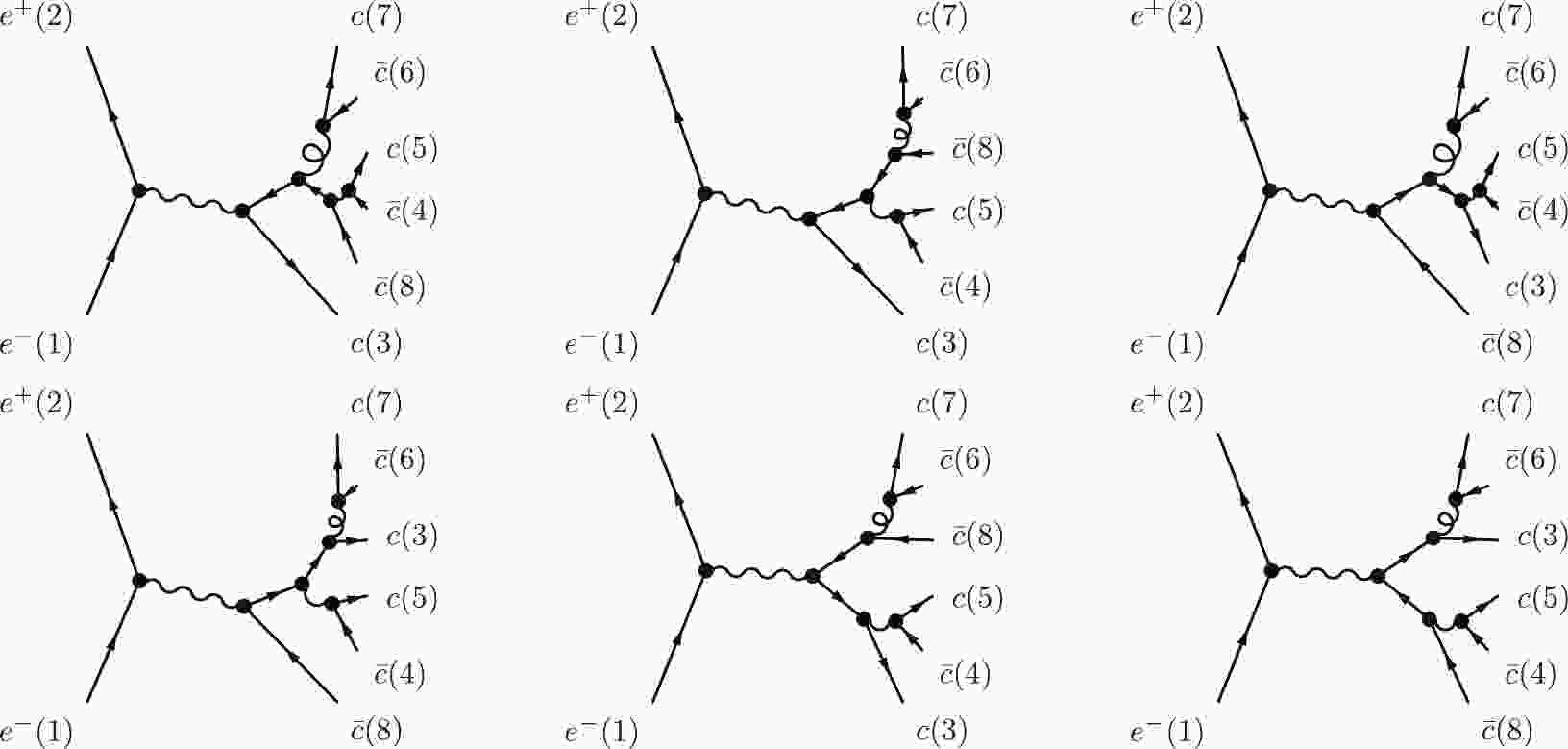
$ e^+e^-\rightarrow c\bar{c}c\bar{c}c\bar{c} $ , as shown in Fig. 1.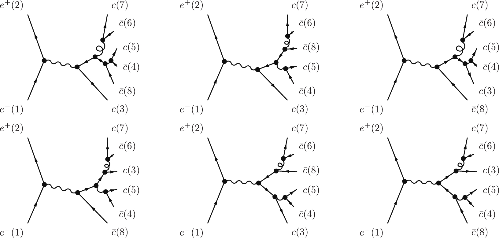
Figure 1. Selected Feynman diagrams of
$ e^+e^-\rightarrow c\bar{c}c\bar{c}c\bar{c} $ in the comparison with WHIZARD. The vector boson coupled with$ e^+e^- $ can be a photon or Z boson.The comparison was conducted in a similar manner, and the results are shown in Table 2. Since both FDC and WHIZARD can provide the expected time for a certain number of events directly, the time for 10000 events were used this time. Meanwhile, the first two processes are marked with
$ g^*\rightarrow b\bar{b} $ and$ g^*\rightarrow c\bar{c} $ , respectively.$ \sqrt{s} $ /GeV

$ e^{+}e^{-}\rightarrow b\bar{b}c\bar{c} $ (

$ g^*\rightarrow b\bar{b} $ )

$ e^{+}e^{-}\rightarrow b\bar{b}c\bar{c} $ (

$ g^*\rightarrow c\bar{c} $ )

$ e^+e^-\rightarrow c\bar{c}c\bar{c}c\bar{c} $ 

FDC WHIZARD FDC WHIZARD FDC WHIZARD 20 0.3 4 0.3 5 7.1 319 50 0.3 5 0.3 7 7.0 760 100 0.3 6 0.3 6 6.8 3935 200 0.2 8 0.3 9 6.8 6999 500 0.2 8 0.3 9 7.1 7905 1000 0.2 11 0.4 10 7.0 6277 Table 2. Expected time to generate 10000 events in unit of seconds.
The table shows that in the
$ 2\rightarrow 4 $ process, FDC is more than 13 times faster than WHIZARD, while in the$ 2\rightarrow 6 $ process, FDC is dozens to hundreds of times faster.Note added: After this work was submitted, a direct comparison on the computation of pure amplitude square with WHIZARD was conducted, with aid from its authors [42]. A slight difference was observed in the time cost of both packages for this part. The large difference observed in Table 2 may result from other parts, such as phase space integrations and event generations.
From both comparisons, we can conclude that with the new algorithm, FDC provides a very good performance in the processes with multiple fermion lines.
-
In this paper, a new approach for the numerical calculation of fermion lines at the tree level is introduced. By calculating two vectors recursively without any matrix multiplications, the result of a fermion line is reduced to a very compact form that depends only on these two vectors. Furthermore, the results for all possible polarization configurations can be obtained simultaneously without extra cost. As shown in the comparisons, FDC provides a very good performance in the processes of multiple fermion lines with this new approach and some other improvements. A further comparison with WHIZARD shows that this new approach has a competitive efficiency in computing pure amplitude squares without phase space integration.
-
We would like to thank Wolfgang Kilian, Thorsten Ohl and Jürgen Reuter for their help in the comparison with WHIZARD.
New approach for amplitudes with multiple fermion lines
- Received Date: 2022-03-29
- Available Online: 2022-08-15
Abstract: A new approach for tree-level amplitudes with multiple fermion lines is presented. It primarily focuses on the simplification of fermion lines. By calculating two vectors recursively without any matrix multiplications, the result of a fermion line is reduced to a very compact form depending only on the two vectors. Comparisons with other packages are presented, and the results show that our package FDC provides a very good performance in the processes of multiple fermion lines with this new approach and some other improvements. A further comparison with WHIZARD shows that this new approach has a competitive efficiency in computing pure amplitude squares without phase space integration.


 DownLoad: