


 Abstract
 HTML
HTML Reference
 Related
 PDF
PDF


-
Measurements of the initial c-quark polarization in charmed-baryon decays play an important role in the search for new physics processes, for example, at the Large Hadron Collider (LHC) experiment. Analysis of spin transfer provides access to the nonperturbative QCD parameters relevant to the dynamics of the hadronization process and thus provides crucial information about the structure of new physics [1, 2]. Moreover, measurement of charmed baryon polarization can be used to search for the anomalous magnetic moment [3], magnetic dipole moments [4], and electromagnetic dipole moments [5–7] at the LHC experiment.
The decay
$ {\Lambda_c^+}\to{pK^-\pi^+} $ can be selected as a spin polarimeter to analyze charmed baryon polarization [1]. Although two-body decays, such as$ {\Lambda_c^+}\to \Lambda\pi^+,\; \Sigma^+\pi^0,\; \Sigma^0\pi^+ $ , and$ pK_S $ , having approximately 1%$ \sim $ 2% branching fractions [8, 9], and their decay asymmetry parameters have recently been well measured [10], their individual branching fractions are only one sixth of that for$ {\Lambda_c^+}\to{pK^-\pi^+} $ . The charged final states can be directly identified in the LHC experiment, and an analysis on the decay$ {\Lambda_c^+}\to{pK^-\pi^+} $ is ongoing [11].Knowledge on spin transfer in the
$ {\Lambda_c^+} \to {pK^-\pi^+} $ decay is essential for calibrating it as a polarimeter in experiments. In the quark model, the lightest charmed baryon,$ {\Lambda_c^+} $ , is composed of$ udc $ quarks and is classified into a mixed-symmetry 20 multiplet; hence, its spin is assigned as$ {{1/2}} $ [8]. Confirmation of the spin-1/2 assignment dates back to the 90s in the NA32 experiment [12]. Owing to limited$ {\Lambda_c^+}\to{pK^-\pi^+} $ events, the spin was not conclusively determined; however, the results were compatible with the spin-1/2 assignment. Recently, using the events from$ {e^+e^-} \to {\Lambda_c^+}{\bar \Lambda_c^-} $ with$ {\Lambda_c^+}\to pK_S,\; \Lambda\pi^+,\; \Sigma^0\pi^+ $ , and$ \Sigma^+\pi^0 $ , the spin-1/2 assignment was confirmed with a significance of approximately 6σ [13].In this study, we propose to calibrate the
$ {\Lambda_c^+} $ polarimeter using the decays$ {e^+e^-}\to{\Lambda_c^+}{\bar \Lambda_c^-} $ and$ {\Lambda_c^+}\to{pK^-\pi^+} $ . These decays were once used to measure the absolute branching fraction of$ {\Lambda_c^+}\to{pK^-\pi^+} $ during the BESIII experiments [14]. Other than its large branching fraction, an advantage is that its polarization information is unambiguously known from the transfer of the unpolarized beams of the$ {e^+e^-} $ collider. The possible existence of$ {\Lambda_c^+} $ transverse polarization (TP) can be determined using data events and is helpful for calibrating the$ {\Lambda_c^+} $ polarimeter.Copious intermediate states, for example,
$ \bar K^*(892)^0 $ ,$ \Delta(1232) $ , and the excited$ \Lambda^* $ and$ \Sigma^* $ states, are observed in the Dalitz plot of the weak decay$ {\Lambda_c^+}\to{pK^-\pi^+} $ [15, 16]. An amplitude model can be applied to the decay to study the decay dynamics [17]. However, a measurement of charmed-baryon polarization requires an analysis of the angular distributions of decayed particles in experiments. The possibility of using$ {\Lambda_c^+}\to{pK^-\pi^+} $ as a spin polarimeter has been demonstrated in [17] with an amplitude model determined via full phase space amplitude analysis. In this study, a model-independent method is developed for the three-body decay$ {\Lambda_c^+}\to{pK^-\pi^+} $ to calibrate it with data events from the spin polarimeter used in other experiments. -
We consider the decay
$ {\Lambda_c^+}(p_0,\lambda_0)\to p(p_1,\lambda) K^-(p_2) \pi^+(p_3) $ using an isobar model. It proceeds via a two-step sequential decay, where$ p_i\;(i=0,1,2,3) $ denote the momenta of individual particles,$ \lambda_0 $ denotes the z-projection of the$ {\Lambda_c^+} $ spin, and$ \lambda_1 $ denotes the proton helicity. Currently, the measurement shows that the resonances$ \Delta(1232)^{++}, \bar{K}^*(890)^0 $ , and$ \Lambda(1520) $ dominate the decays. Their branching fractions add up to 5.2%, as shown in Table 1, whereas the total branching fraction for$ {\Lambda_c^+}\to {pK^-\pi^+} $ is measured to be (6.23$ \pm $ 0.23)%.$ {\Lambda_c^+}\to $ 

Branching fraction Vertex form $ \Delta(1232)^{++}K^- $ 

(1.07 $ \pm $ 0.25)%

$ f_1\gamma_5p_0^\mu+f_2p_0^\mu $ 

$ \Lambda(1520)\pi^+ $ 

(2.2 $ \pm $ 0.5)%

$ f_3p_0^\mu+f_4\gamma_5p_0^\mu $ 

$ p\bar{K}^*(892)^0 $ 

(1.94 $ \pm $ 0.27)%

$ f_5p_0^\mu+f_6\gamma_\mu $ 

$ +f_7(p_2^\nu+p_3^\nu)\sigma_{\mu\nu} $ 

$ +\gamma_5(f_8p_0^\mu+f_9\gamma_\mu) $ 

$ +\gamma_5f_{10}(p_2^\nu+p_3^\nu)\sigma_{\mu\nu} $ 

$ \Delta^{++}\to p\pi^+ $ 

33.1% $ f_8p_{1\mu} $ 

$ \Lambda(1520)\to pK^- $ 

22.5% $ f_9\gamma_5p_{1\mu} $ 

$ \bar{K}^*(892)^0\to K^-\pi^+ $ 

33.3% $ f_{11}p_{2\mu} $ 

Table 1. Branching fractions and the vertex forms of the decay for resonances in
$ {\Lambda_c^+}\to{pK^-\pi^+}.$ The Dalitz-plot decomposition of the
$ {\Lambda_c^+}\to{pK^-\pi^+} $ decay has been discussed with the helicity amplitude in Ref. [18]. In this study, we construct the amplitudes for these two-step consequential decays using the covariant tensor formalism, which is then related to the calculation of the helicity amplitude. The first-step decay occurs by emitting a W boson from a charmed quark and changing the charmed quark into a strange quark. This decay induces a weak interaction, and the decay does not conserve parity. The vertex forms of the tensor formalism, which include parity-violation terms, are given in Table 1 in terms of the linear combination with complex numbers$ f_i\;(i=1,2,..,10) $ . The second-step decays of intermediate states conserve spin and parity, and their vertex forms are also given in Table 1. To calculate the amplitudes, we present the amplitude for the sequential decay in the helicity system.The helicity amplitudes for
$ {\Lambda_c^+}(p_0,\lambda_0)\to \Delta(1232)^{++}K^- \to p(p_1,\lambda_1)K(p_2)\pi^+(p_3) $ reads as$ \begin{aligned}[b] F^\Delta_{\lambda_0,\lambda_1}(m_{p\pi^+})=&{\rm{Tr}}\Big[ u_{\lambda_0}(p_0)\bar{u}_{\lambda_1}(p_1)p_0^\mu(f_1\gamma_5+f_2)\\ &\times S^{3/2}_{\mu\nu}(p_1+p_3,m_{\Delta},\Gamma_{\Delta})f_8p_{1}^\nu\Big], \end{aligned} $

(1) where
$ u_{\lambda}(p) $ is the Dirac spinor, normalized with$ \bar u u=2m $ , and$ \lambda_0(\lambda_1) $ is the helicity value for the$ {\Lambda_c^+}(p) $ particle, that is,$ \begin{aligned}[b] u_{\lambda}(p) =& {\not p+m\over \sqrt{p^0+m}}u_\lambda(0),{\; {\rm{with}}\; }\\ u_{+{1/2}}(0)=&\left(\cos{\theta\over 2},\sin{\theta\over 2}{\rm e}^{{\rm i}\phi},0,0\right)^T,\\ u_{-{1/ 2}}(0)=&\left(-\sin{\theta\over 2}{\rm e}^{-{\rm i}\phi},\cos{\theta\over 2},0,0\right)^T, \end{aligned} $

(2) where
$ \theta,\phi $ are the polar and azimuthal angles of the momentum in the Dirac spinor, respectively.$ S^{3/2}_{\mu\nu} $ is the propagator for$ \Delta(1232) $ , which is given in Appendix B. In this decay, the two terms with the coupling constants$ f_1 $ and$ f_2 $ correspond to the violated and conserved parity contributions, respectively.Similarly, the helicity amplitude for
$ {\Lambda_c^+}\to \Lambda(1520)\pi^+ \to{pK^-\pi^+} $ can be expressed as$ \begin{aligned}[b] F^\Lambda_{\lambda_0,\lambda_1}(m_{pK^-})=&{\rm{Tr}}\Big[u_{\lambda_0}(p_0)\bar{u}_{\lambda_1}(p_1)p_0^\mu(f_3+f_4\gamma_5)\\ &\times S^{3/2}_{\mu\nu}(p_1+p_2,m_{\Lambda},\Gamma_{\Lambda})f_9p_{1}^\nu\Big], \end{aligned} $

(3) where
$ S^{3/2}_{\mu\nu} $ is the propagator for$ \Lambda(1520) $ . In this decay, the two terms with the coupling constants$ f_3 $ and$ f_4 $ correspond to the violated and conserved parity contributions, respectively.The helicity amplitude for
$ {\Lambda_c^+}\to p\bar{K}^*(892)^0 \to {pK^-\pi^+} $ can be expressed as$ \begin{aligned}[b] F^{K^*}_{\lambda_0,\lambda_1}(m_{K^-\pi^+})=&{\rm{Tr}}\Big[u_{\lambda_0}(p_0)\bar{u}_{\lambda_1}(p_1)\\ &\times[f_5p_0^\mu+f_6\gamma_\mu+f_7(p_2^\nu+p_3^\nu)\sigma_{\mu\nu}\\ &+\gamma_5(f_8p_0^\mu+f_9\gamma_\mu+f_{10}(p_2^\beta+p_3^\beta)\sigma_{\mu\beta})\Big]\\ &\times S^1_{\mu\alpha}(p_2+p_3,m_{K^*},\Gamma_{K^*})f_{11}p_2^\alpha, \end{aligned} $

(4) where
$ S^{1}_{\mu\alpha} $ is the propagator for$ \bar{K}^*(892)^0 $ , which is given in Appendix B. In this decay, the terms combined with the coupling constants$ f_8,\;f_9 $ , and$ f_{10} $ correspond to the parity-violation contributions, while the terms combined with$ f_5,\;f_6 $ , and$ f_7 $ correspond to the parity-conserved contributions. -
The spin of
$ {\Lambda_c^+} $ is conclusively determined to be 1/2, and its spin density matrix (SDM) can be expressed with a$ 2\times 2 $ matrix. This is usually written in terms of Pauli σ matrices as$ \rho({\Lambda_c^+}) = {\frac{1}{ 2}} (1+\vec{\mathcal{P}}\cdot {\vec\sigma})={\frac{1}{2}}\left[ \begin{matrix} 1+\mathcal{P}_z & \mathcal{P}_x-{\rm i}\mathcal{P}_y\\ \mathcal{P}_x+{\rm i}\mathcal{P}_y & 1-\mathcal{P}_z \end{matrix} \right] , $

(5) where the mean polarization vector
$ \vec{\mathcal{P}}=(\mathcal{P}_x,\mathcal{P}_y,\mathcal{P}_z) $ , which determines the$ {\Lambda_c^+} $ polarization.For the
$ {\Lambda_c^+}(\lambda_0)\to p(\lambda_1)K^+\pi^- $ decay, the three final-state particles are located on the same decay plane in the rest frame of the$ {\Lambda_c^+} $ system. We take the x axis to be along the proton flying direction, the z axis is the normal to the decay plane, and the y axis is vertical to the$ xz $ plane; hence, they form a right-hand system. The orientation of this system is described using three Euler angles ($ \alpha,\beta,\gamma $ ), with which the three successive rotations carry the$ {\Lambda_c^+} $ production helicity system to this system. The SDM of the proton can be calculated using$ \rho(p)=N\cdot\rho({\Lambda_c^+})\cdot N^\dagger, $

(6) where N is a
$ {\Lambda_c^+} $ decay matrix, which can be expressed as$ N_{\lambda_1,\lambda_0}=\sum\limits_{\mu=\pm1/2} D^{1/2*}_{\lambda_0,\;\mu}(\alpha,\beta,\gamma)F_{\mu,\,\lambda_1}(m_{pK},m_{p\pi},m_{K\pi}), $

(7) where the decay matrix
$ F_{\mu,\,\lambda_1} $ is dependent on the resonance structures in the$ {pK^-\pi^+} $ final states, which can be expressed by the coherent sum of intermediate states, as given in the previous section; that is,$ \begin{aligned}[b] |F_{\mu,\lambda_1}(m_{pK},m_{p\pi},m_{K\pi})|^2=&|F^{\Delta}_{\mu,\lambda_1}(m_{p\pi^+})\\ &+F^{\Lambda}_{\mu,\lambda_1}(m_{pK^-})+F^{K^*}_{\mu,\lambda_1}(m_{K^-\pi^+})|^2. \end{aligned} $

(8) For a study on intermediate states in
$ {\Lambda_c^+} $ decays,$ F_{\mu,\lambda_1} $ must be related to the decay amplitude of different resonances observed in the$ {pK^-\pi^+} $ final states [18]. In this study, we do not model the decay matrix$ F_{\mu,\lambda_1} $ . Instead we treat it as a model-independent parameter and then relate them to the polarization parameters; the values can be determined with the data events. This treatment has the advantage of model-independent measurement on the$ {\Lambda_c^+} $ polarization parameters.Because the helicity amplitudes are isolated from the angular distributions represented by Euler angles, we can integrate out the masses in the above model-dependent amplitude over the three body space
$ {\rm d}\Phi_3 $ . It then relates to the square of the model-independent amplitude,$ |F_{\mu,\lambda_1}|^2=\int {\rm d}\Phi_3 |F_{\mu,\lambda_1}(m_{pK},m_{p\pi},m_{K\pi})|^2, $

(9) where the invariant masses,
$ m_{pK},\;m_{p\pi} $ , and$ m_{K\pi} $ , are treated as Dalitz plot variables, and only two are independent in the integral. Because the mass variables are integrated out, we will suppress this mass dependence of the helicity amplitudes in what follows.In practice, integration over the phase space can be estimated as an average using the Monte-Carlo method. If the number of unweighted phase-space Monte-Carlo (MC) events is sufficiently large, the helicity amplitude can be estimated as
$ |F_{\mu,\lambda_1}|^2={\widetilde{\Phi_3}\over N}\sum_{i=1}^N|F_{\mu,\lambda_1}(m_{pK},m_{p\pi},m_{K\pi})|^2, $

(10) where
$ m^{(i)}_{p\pi^+},\; m^{(i)}_{pK^-} $ , and$ m^{(i)}_{K^-\pi^+} $ are invariant masses calculated with the i-th phase-space event, and$ \widetilde{\Phi_3}=\int {\rm d}\Phi_3 $ is the normalization factor when generating the unweighted MC events.The angular distribution of protons can be calculated by taking the trace of its SDM matrix.
$ \mathcal{W}(\alpha,\beta,\gamma)=\mathcal{A}_0 + \mathcal{\vec P}\cdot \mathcal{\vec A}, $

(11) where
$ \mathcal{A}_0 $ corresponds to an unpolarized cross section, and$ \mathcal{\vec A} $ represents the analyzing power. These are determined with the$ {\Lambda_c^+} $ decay matrix as①$ \mathcal{A}_0 ={\rm{Tr}}[N\cdot N^\dagger], $

(12) $ \mathcal{\vec A}={\rm{Tr}}[N\cdot\vec\sigma\cdot N^\dagger]. $

(13) Using the
$ {\Lambda_c^+} $ decay matrix, we get$ \begin{aligned}[b] \mathcal{A}_0 =&|F_{-{{1/ 2}},-{{1/ 2}}}|^2+|F_{-{{1/ 2}},{{1/ 2}}}|^2+|F_{{{1/ 2}},-{{1/ 2}}}|^2+|F_{{{1/ 2}},{{1/ 2}}}|^2,\\ \mathcal{A}_x =&2 \left(\mathcal{I}_1+\mathcal{I}_2\right) (\sin \alpha \cos \gamma -\cos \alpha \cos \beta \sin \gamma )\\ &+2(\mathcal{R}_1+\mathcal{R}_2)(\cos \alpha \cos \beta \cos \gamma +\sin \alpha \sin \gamma )\\ &+\mathcal{G} \cos \alpha \sin \beta ,\\ \mathcal{A}_y=&-2 (\mathcal{I}_1+\mathcal{I}_2) (\sin \alpha \cos \beta \sin \gamma +\cos \alpha \cos \gamma )\\ &+2 (\mathcal{R}_1+\mathcal{R}_2) (\sin \alpha \cos \beta \cos \gamma -\cos \alpha \sin \gamma )\\ &+\mathcal{G} \sin \alpha \sin \beta ,\\ \mathcal{A}_z =&2 \left(\mathcal{I}_1+\mathcal{I}_2\right) \sin \beta \sin \gamma +\mathcal{G} \cos \beta \\ &-2 \left(\mathcal{R}_1+\mathcal{R}_2\right) \sin \beta \cos \gamma. \end{aligned} $

(14) Here, we define
$ \begin{array}{*{20}{l}} \mathcal{G} =\big|F_{{{1/ 2}},-{{1/ 2}}}\big|^2+\big|F_{{{1/ 2}},{{1/ 2}}}\big|^2-\big|F_{-{{1/ 2}},-{{1/ 2}}}\big|^2-\big|F_{-{{1/ 2}},{{1/ 2}}}\big|^2. \end{array} $

If parity is conserved in
$ {\Lambda_c^+}\to{pK^-\pi^+} $ ,$\mathcal{G}= 2\big|F_{{1/ 2},{1/ 2}}\big|^2- 2\big|F_{-{1/ 2},-{1/ 2}}\big|^2$ .$ \mathcal{R}_1 $ and$ \mathcal{I}_1 $ are the real and imaginary parts of the product of the amplitudes,$F^{*}_{{1}/{2},-{1}/{2}} F_{-{1}/{2},-{1}/{2}}$ , respectively, while$ \mathcal{R}_2 $ and$ \mathcal{I}_2 $ are those of the product$ F^*_{{1}/{2},{1}/{2}}F_{-{1}/{2},{1}/{2}} $ . These are determined using the square of the helicity amplitude, for instance,$ \begin{aligned}[b] 2\mathcal{R}_1=&\int {\rm d}\Phi_3\left[\big|F_{{1}/{2},-{1}/{2}}(...)+F_{-{1}/{2},-{1}/{2}}(...)\big|^2-\big|F_{{1}/{2},-{1}/{2}}(...)\big|^2-\big|F_{-{1}/{2},-{1}/{2}}(...)\big|^2\right],\\ 2\mathcal{I}_1=&\int {\rm d}\Phi_3\left[\big|F_{{1}/{2},-{1}/{2}}(...)\big|^2-\big|F_{-{1}/{2},-{1}/{2}}(...)\big|^2-\big|F_{{1}/{2},-{1}/{2}}(...)+{\rm i}*F_{-{1}/{2},-{1}/{2}}(...)\big|^2\right], \end{aligned} $ 
(15) where
$ (...) $ implies the integration variables$(m_{pK},m_{p\pi}, m_{K\pi})$ , as given in Eq. (8). These are dependent on the coupling constants$ f_i $ , as shown in Table 1.In the above equations,
$ \mathcal{A}_0 $ corresponds to the unpolarized cross section of$ {\Lambda_c^+} $ decays, while$ \mathcal{R}_{1,2} $ ,$ \mathcal{I}_{1,2} $ , and$ \mathcal{G} $ correspond to contributions due to parity violation. We introduce three parameters characterizing the asymmetric distribution of$ {\Lambda_c^+} $ decays into$ {pK^-\pi^+} $ final states, namely,$ \mathcal{G}_0 = \mathcal{G}/\mathcal{A}_0, \quad \mathcal{G}_1=(\mathcal{I}_1+\mathcal{I}_2)/\mathcal{A}_0,\quad \mathcal{G}_2=(\mathcal{R}_1+\mathcal{R}_2)/\mathcal{A}_0,\nonumber $

and reformulate the angular distribution as
$ \mathcal{W}(\alpha,\beta,\gamma)=\mathcal{A}_0[1+\mathcal{G}_0\mathcal{\vec P}\cdot \mathcal{\vec R}+\mathcal{G}_1\mathcal{\vec P}\cdot \mathcal{\vec S}+\mathcal{G}_2\mathcal{\vec P}\cdot \mathcal{\vec T}], $

(16) where
$ \vec{\mathcal{P}} $ is the$ {\Lambda_c^+} $ polarization vector,$ \begin{aligned}[b] \vec{\mathcal{P}}=&(\mathcal{P}_x,\mathcal{P}_y,\mathcal{P}_z),\\ \vec{\mathcal{R}}=&(\sin\beta\cos\alpha,\sin\beta\sin\alpha,\cos\beta),\\ \vec{\mathcal{S}}=&(\sin \alpha \cos \gamma -\cos \alpha \cos \beta \sin \gamma ,\\ &-\sin \alpha \cos \beta \sin \gamma -\cos \alpha \cos \gamma,\\ &\sin \beta \sin \gamma)\\ \vec{\mathcal{T}}=&(\cos \alpha \cos \beta \cos \gamma +\sin \alpha \sin \gamma,\\ &\sin \alpha \cos \beta \cos \gamma -\cos \alpha \sin \gamma,\\ &- \sin \beta \cos \gamma). \end{aligned} $

(17) If the angle γ is integrated out, the angular distribution is reduced to
$ \mathcal{W}(\alpha,\beta)= \mathcal{A}_0[1+{\mathcal{G}_0}\vec{\mathcal{P}}\cdot\vec{\mathcal{R}}]. $

(18) In the above equations, the parameters
$ \mathcal{G}_0,\; \mathcal{G}_1 $ , and$ \mathcal{G}_2 $ are determined by the intrinsic properties of the decays, in which the parity is not conserved in the production of intermediate states, such as$ \Delta(1232),\; \Lambda(1520) $ and$ \bar{K}^{*}(892) $ . If we observe the distribution of the angle between, for example,$ \vec{\mathcal{P}} $ and$ \vec{\mathcal{R}} $ , the slope of the asymmetry angular distribution is proportional to$ \vec{\mathcal{G}}_0 $ . In this sense, labeling them as asymmetry parameters is a direct generalization for a two-body decay, for instance,$ \Lambda\to p\pi^- $ . If the parity is conserved,$ F_{1/2,1/2}=-F_{1/2,-1/2} $ ,$ F_{-1/2,1/2}=F_{-1/2,-1/2} $ , and$ F_{-1/2,1/2}= F_{1/2,-1/2} $ . This leads to$ \mathcal{G}_0=0 $ .In experiments,
$ {\Lambda_c^+} $ polarization can be determined by measuring several moments, which are defined as the average of the polarization observables, formed with Euler angles. Some of the moments related to the polarization vector are listed below.$ \begin{aligned}[b] \mathcal{P}_x&={3\langle \cos\alpha\sin\beta\rangle/\mathcal{G}_0},\quad \mathcal{P}_y={3\langle \sin\alpha\sin\beta\rangle/\mathcal{G}_0},\\ \mathcal{P}_z&={3\langle \cos\beta\rangle/\mathcal{G}_0}. \end{aligned} $

(19) Here, we consider the factor
$ \mathcal{G}_0={\mathcal{G}/\mathcal{A}_0} $ to be the asymmetry parameter with the assumption$ \mathcal{G}\neq 0 $ , which is intrinsically determined by the helicity amplitudes of the$ {\Lambda_c^+}\to {pK^-\pi^+} $ decay. Once it is determined in one experiment, it is applicable to other experiments for measurements of$ {\Lambda_c^+} $ polarization. -
The sensitivity of measurement on the asymmetry parameter,
$ \mathcal{G}_0={\mathcal{G}/ \mathcal{A}_0} $ , is determined by the number of$ {\Lambda_c^+} $ events. We define the sensitivity as$ \delta\mathcal{G}_0={\sqrt{V(\mathcal{G}_0)}\over \mathcal{G}_0}, $

(20) where
$ V(\mathcal{G}_0) $ is the variance of$ \mathcal{G}_0 $ , which is estimated with the likelihood function. For a sample with N events,$ X_1,X_2,..., X_N $ , the likelihood function$ \mathcal{L} $ defined over the parameters$ \mathcal{G}_0 $ is given by$ \mathcal{L}(X_1,X_2,...,X_N|\mathcal{G}_0)=\prod_{i=1}^N \widetilde{\mathcal{W}}(X_i|\mathcal{G}_0), $

(21) where
$ \widetilde{\mathcal{W}}=\mathcal{W}(\alpha,\beta)/\int \mathcal{W}(\alpha,\beta)\sin\beta {\rm d}\beta {\rm d}\alpha $ is the normalized function of the angular distribution (see Eq. (18)). With the maximum likelihood estimate, the variance of parameter$ \mathcal{G}_0 $ is defined by the expected value.$ \begin{aligned}[b] V^{-1}(\mathcal{G}_0)=&E\left[-{\partial^2\ln\mathcal{L}(X_i|\mathcal{G}_0)\over \partial^2\mathcal{G}_0}\right],\\ =&N\int {1\over \widetilde{\mathcal{W}}}\left[{\partial \widetilde{\mathcal{W}}(X|\mathcal{G}_0)\over \partial \mathcal{G}_0} \right]^2 {\rm d}X, \end{aligned} $

(22) where
$ {\rm d}X=\sin\beta {\rm d}\beta {\rm d}\alpha $ .We consider a special case with weak polarization and a small asymmetry parameter
$ \mathcal{G}_0 $ , such that$ \mathcal{G}_0 |\vec{\mathcal P}| \ll1 $ . In particular, the$ {\Lambda_c^+} $ events are accumulated at the$ {e^+e^-} $ collider near the$ {\Lambda_c^+}{\bar \Lambda_c^-} $ mass threshold in the BESIII experiment [10], with$ \mathcal{P}_x=\mathcal{P}_z=0 $ . Up to an accuracy of$ \mathcal{O}((\mathcal{G}_0 |\vec{\mathcal P}|)^5) $ , we obtain$ \delta \mathcal{G}_0 = \sqrt{105\over N}{1\over\mathcal{G}_0\mathcal{P}_y }{ \sqrt{1\over35+21\mathcal{G}_0^2\mathcal{P}_y^2+15\mathcal{G}_0^4\mathcal{P}_y^4}}. $

(23) An inverse problem in the application of the spin polarimeter concerns the estimation of the polarization measurement sensitivity, which can be determined using the same procedure. We find that it has the same form as the
$ \mathcal{G}_0 $ measurement because the polarization is solely dependent on the$ \mathcal {G}_0 $ measurement, as shown in Eq. (19), namely,$ {\Delta \mathcal{P}_y\over \mathcal{P}_y} = \sqrt{105\over N}{1\over\mathcal{G}_0\mathcal{P}_y }{ \sqrt{1\over35+21\mathcal{G}_0^2\mathcal{P}_y^2+15\mathcal{G}_0^4\mathcal{P}_y^4}}. $

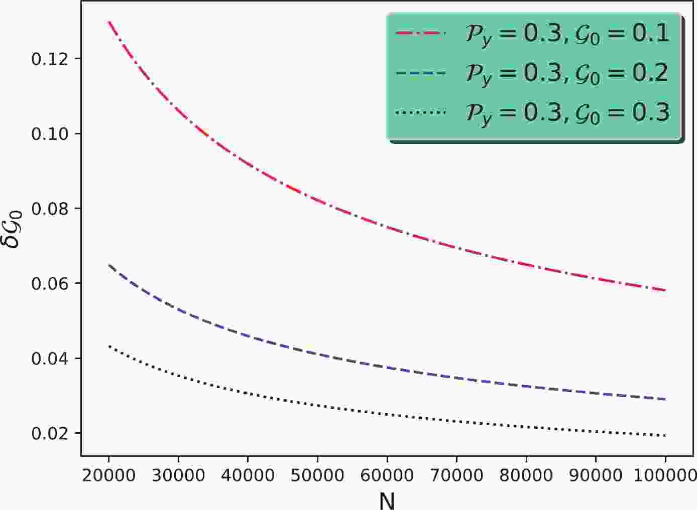
(24) Estimation of the sensitivity is dependent on the measurements of parameters
$ \mathcal{P} $ and$ \mathcal{G}_0 $ . Figure 1 shows that the sensitivities of measurement$ \delta\mathcal{G}_0 $ varied with the number of$ {\Lambda_c^+} $ candidates for the different parameters, for instance,$ \mathcal{P}_y=0.3 $ and$ \mathcal{G}_0=0.1,0.2,0.3 $ . Here, we assume the use of an$ {e^+e^-} $ collider with unpolarized beams and$ \mathcal{P}_x=\mathcal{P}_z=0 $ , such as in the BESIII experiment. We can see that a sensitivity of a few percent can be achieved if$ 10^5 ~{\Lambda_c^+} $ candidates survive from the event selection criteria.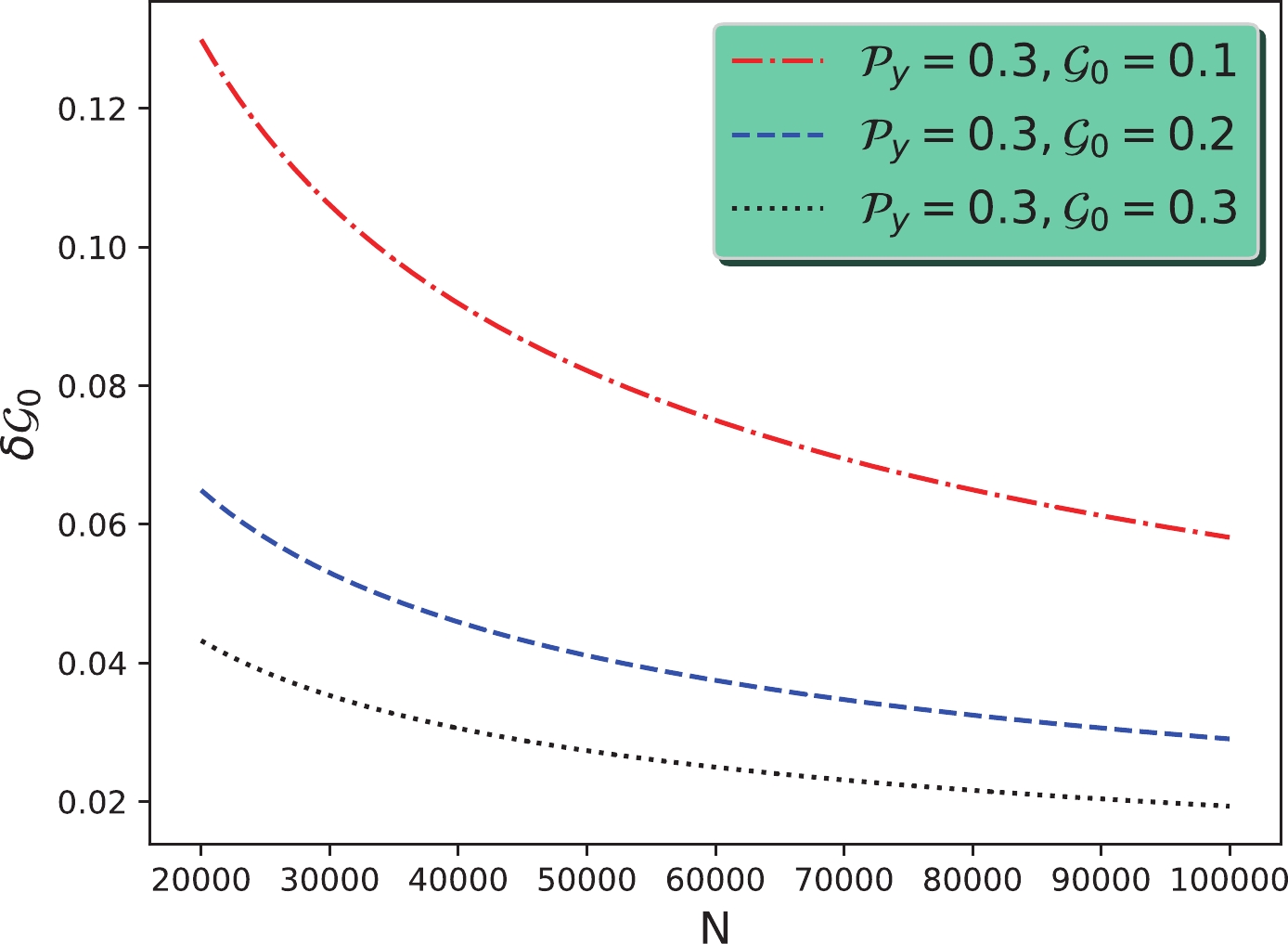
Figure 1. (color online) Sensitivity of measurement
$ \delta\mathcal{G}_0 $ for the different parameters$ \mathcal{P}_y $ and$ \mathcal{G}_0 $ with the decay$ {\Lambda_c^+}\to{pK^-\pi^+} .$ -
The advantages of calibrating the
$ {\Lambda_c^+} $ polarimeter with$ {e^+e^-} $ annihilation events originate from the parity conservation in this electromagnetic process. Also,$ {\Lambda_c^+} $ polarization is well known. For the unpolarized$ {e^+e^-} $ beam experiment, a virtual photon is produced from$ {e^+e^-} $ annihilation with tensor polarization, while the longitudinal polarization is zero. Hence, the polarization of$ {\Lambda_c^+} $ particles is only allowed along the direction normal to the$ {\Lambda_c^+} $ production plane.To calculate the
$ {\Lambda_c^+} $ SDM, we first define the$ {\Lambda_c^+} $ helicity system (x-y-z), which is produced from the$ {e^+e^-}\to{\Lambda_c^+}(\lambda_1){\bar \Lambda_c^-}(\lambda_0) $ process, as shown in Fig. 2. The z axis is taken along the$ {\Lambda_c^+} $ flying direction, the x axis is defined in the$ {\Lambda_c^+} $ -production plane formed by the$ e^+ $ beam and$ {\Lambda_c^+} $ momenta and is normal to the$ {\Lambda_c^+} $ momentum, and the y axis is taken along the normal to the$ {\Lambda_c^+} $ -production plane; therefore,$ x,y,z $ form a right-hand system. In the$ {e^+e^-} $ -center-of-mass (CM) system, the$ {\Lambda_c^+} $ momentum is characterized by the polar angle θ. Then, the$ {\Lambda_c^+} $ SDM is calculated using
Figure 2. (color online) Definition of the
$ {\Lambda_c^+} $ helicity system for its production from the$ {e^+e^-}\to{\Lambda_c^+}{\bar \Lambda_c^-},{\Lambda_c^+}\to{pK^-\pi^+} $ process.$ \begin{aligned}[b] \rho({\Lambda_c^+})_{\lambda_1,\lambda'_1}=&\sum_{m,\lambda_0} D^{1*}_{m,\lambda_1-\lambda_0}(0,\theta,0)\\ &\times D^{1}_{m,\lambda'_1-\lambda_0}(0,\theta,0)A_{\lambda_1,\lambda_0}A^*_{\lambda'_1,\lambda_0}, \end{aligned} $

(25) where
$ m=\pm1 $ is the spin projection of the virtual photon, and$ A_{\lambda_1,\lambda_2} $ denotes the helicity amplitudes. There are two independent amplitudes due to the constraints of parity conservation, that is,$ A_{-{1/ 2},\,-{1/ 2}}=A_{{1/2},\,{1/2}},\; A_{-{{1/2}},\,{{1/ 2}}}= A_{{{1/ 2}},\,-{{1/2}}} $ . In the experiment, only the ratio of two amplitudes can be measured. The study on the$ {\Lambda_c^+} $ angular distribution is related to the measurement of amplitude ratio, namely,$\alpha_c = \Big(\,\big|A_{{{1/ 2}},\,-{{1/2}}}\big|^2 - 2\big|\,A_{{{1/2}},\,{{1/ 2}}}\big|^2\,\Big)/ \Big(\,\big|\,A_{{{1/2}},\,-{{1/ 2}}}\big|^2+ 2|A_{{{1/ 2}},\,{{1/ 2}}}\,\big|^2\,\Big),$ where$ \alpha_c $ is the angular distribution parameter for the$ {\Lambda_c^+} $ particles. Using these relations, the$ {\Lambda_c^+} $ polarization vector can be expressed as$ \begin{aligned}[b] \mathcal{P}_x&=\mathcal{P}_z=0,\\ \mathcal{P}_y&={\sqrt{1-\alpha_c^2}\sin2\theta\sin\Delta\over 4(1+\alpha_c\cos^2\theta)}, \end{aligned} $

(26) where Δ is the difference between the phase angles in the two independent helicity amplitudes. The nonzero
$ \sin\Delta $ allows us to observe the transverse polarization of$ {\Lambda_c^+} $ production in$ {e^+e^-} $ collisions. Recent measurements have shown that$ {\Lambda_c^+} $ TP is insignificant at energies near the$ {\Lambda_c^+}{\bar \Lambda_c^-} $ mass threshold, with measurements of$ \alpha_c=-0.20\pm0.04\pm0.02 $ [19] and$ \sin\Delta=-0.28\pm0.13\pm 0.03 $ using BESIII data taken at energy point$ \sqrt s=4.6 $ GeV [10]. Although the average of$ {\Lambda_c^+} $ TP vanishes when an estimation is made over full detector coverage, the polarizations in the forward and backward hemisphere of the detector are nonvanishing and have a reverse sign. This allows us to measure the polarization constant$ 3\mathcal{A}_0/\mathcal{G} $ defined in the helicity system. -
We use the Monte-Carlo method to obtain the polarization constant. In a model-dependent analysis, the coupling constants
$ f_i\;(i=1,2,...,10) $ in the helicity amplitudes can be determined by fitting the angular distribution of Eq. (11) to data events by substituting the helicity amplitudes$ F_{\lambda_1,\lambda_2} $ of Eqs. (1)–(4). As an example, to show the simulation of Monte-Carlo event production, we only select the$ {\Lambda_c^+} $ decay to$ p\bar{K}^{*}(892)^0 $ .In the calculation of the three Euler angles, we first boost the
$ p(p_1)K^-(p_2)\pi^+(p_3) $ final states to the$ {\Lambda_c^+} $ rest frame so that$ \vec{p}_1+\vec{p}_2+\vec{p}_3=0 $ , as shown in Fig. 2. We describe$ {\Lambda_c^+} $ decay in the system (X-Y-Z), which defines the orientation of the decay plane formed by the momenta of three$ {pK^-\pi^+} $ final states. The X axis is taken along the proton flying direction, the Z axis is normal to the decay plane [20, 21] and parallel to$ \vec p_1\times \vec p_2 $ , and the Y axis is chosen to form a right-hand system, as shown in Fig. 2. Moreover,$ {\Lambda_c^+} $ polarization is described in the (x-y-z) system (see Fig. 2), as defined in the previous section. For a given event, three successive Euler rotations must be performed so that the$ (x $ -y-$ z) $ system is carried to overlap the (X-Y-Z) frame, as shown in Fig. 3. First, angle α is rotated about the z-axis to align the y-axis along the nominal to the plane formed by$ {\boldsymbol z\times \boldsymbol Z} $ . Then, angle β is rotated about the y-axis to align$ {\boldsymbol z} $ to the$ {\boldsymbol Z} $ direction. Finally, angle$ {\boldsymbol \gamma} $ is rotated about the Z axis to overlap the two systems. The angles$ (\beta,\alpha) $ correspond to the polar and azimuthal angles of the z axis in the (X-Y-Z) system. The calculation of Euler angles is given in Appendix A.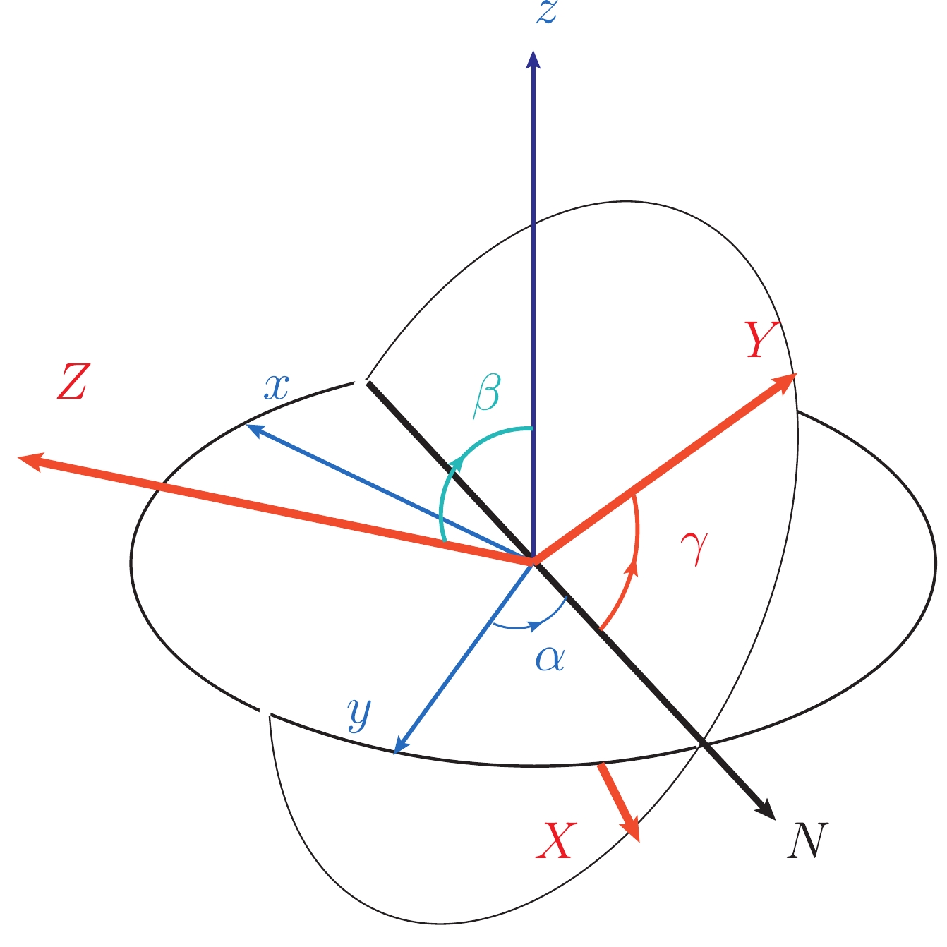
Figure 3. (color online) Euler rotations to overlap the
$ {\boldsymbol(x,y,z)} $ system with the$ {\boldsymbol (X,Y,Z)} $ system using angles$ (\alpha,\beta,\gamma) $ for the decay$ {\Lambda_c^+}\to{pK^-\pi^+} .$ In the decay plane, the momenta of the final states are denoted by
$ p_1,\;p_2 $ , and$ p_3 $ , and their z components are zero. The direction of the proton is along the x axis; therefore,$ p_{1x}=|\vec p_1| $ ,$ p_{1y}=0 $ ,$ p_{2x}=\vec p_1\cdot \vec p_2/|\vec p_1| $ ,$ p_{3x}=\vec p_1\cdot \vec p_3/|\vec p_1| $ ,$ p_{2y}=\vec Y\cdot \vec p_{2y} $ , and$ p_{3y}=\vec Y\cdot \vec p_{3y} $ , where$ \vec Y={(\vec Z\times \vec p_1)}/{ |\vec p_1|} $ . Only the ratios of the$ f_i $ coupling constants are measured in the experiment, and we set$ f_5=f_6=f_7=f_8=f_9=f_{10}=1+i $ in the MC event generation. The mass and width of$ \bar{K}^{*}(892)^0 $ are taken as$ m_{K^*}=895.55 $ MeV and$ \Gamma_{K^*}=47.3 $ MeV, respectively. Figure 4 shows the events sampled using the acceptance-rejection method.$ \bar{K}^*(892) $ is identified in the$ m_{pK^-} $ spectrum, and the calibration constant is distributed with a peak at approximately$ \mathcal{A}_0/\mathcal{G}=12.0 $ .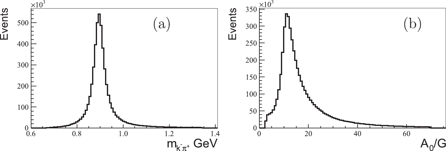
Figure 4.
$ m_{pK^-} $ and$ \mathcal{A}_0/\mathcal{G} $ distribution in the generated Monte-Carlo events.Using a large number of
$ {\Lambda_c^+}\to{pK^-\pi^+} $ events, the averages of the helicity amplitudes squared in Eq. (14) are calculated to be$ \mathcal{R}_1+\mathcal{I}_1{\rm i}=-4.78-1.65{\rm i} $ ,$ \mathcal{R}_2+\mathcal{I}_2{\rm i}=106.14+ 4.96{\rm i} $ , and$ \mathcal{G}_0=11.83/223.93 $ . We consider a general case and set the polarization vector$ \mathcal {\vec P}=(0.0,0.5,0.0) $ . Using an ensemble of generated events, the polarization can be calculated using the moments given in Eq. (19). The statistics of the polarizations are shown in Fig. 5. The two peaks are centered at the input polarization of the$ \mathcal P_y,\;\mathcal P_z $ values and follow Gaussian distributions, with the standard deviation determining the statistical uncertainties. From these distributions, we obtain$ \mathcal{P}_y= 0.494\pm 0.074 $ . From these simulations, the sensitivity of$ \mathcal{P}_y $ , for example, is determined as 15.0%, which is dependent on the values of$ \mathcal P_x,\; N $ , and$ \mathcal G_0 $ . Furthermore, for a consistency check, we can also estimate the sensitivity of$ \mathcal P_y $ to be$ 14.7\% $ using Eq. (24) by substituting in$ \mathcal P_x=0.5, \; N= 200000 $ , and$ \mathcal G_0=11.83/223.93 $ in the Monte-Carlo simulations.
Figure 5. (color online) Distribution of polarizations
$ \mathcal P_y $ (left peak) and$ \mathcal P_z $ (right peak) for 438 sets of MC simulations for the decay$ {\Lambda_c^+}\to{pK^-\pi^+} $ , with 200,000 events for each MC set. -
Measurement of the polarization transfer plays an important role in the search for new physics processes in charmed baryon decays. We show that the decay
$ {\Lambda_c^+}\to {pK^-\pi^+} $ can be chosen as a spin polarimeter. A general description of the decay is developed using Euler angles, and the polarization parameters are derived using a helicity amplitude method. A relationship with parity violation is revealed using the phenomenological amplitude model. A Monte-Carlo simulation is performed, and the results show that charmed baryon polarization can be well separated using a set of Monte-Carlo events with selected asymmetry parameters. The measurement of these asymmetry parameters in experiments is recommended. -
We take an intrinsic rotation starting with the
$ {\Lambda_c^+} $ -helicity system (x-y-z) to reach the target system (X-Y-Z). The unit vectors of the two systems are defined in the$ {\Lambda_c^+} $ -CM system. The unit vectors$ \hat X,\;\hat Y $ , and$ \hat Z $ are defined by the CM momenta of the final states of the$ {\Lambda_c^+}\to p(p_1) K^-(p_2) \pi^+(p_3) $ decay, that is,$ \begin{aligned}[b] \hat X={\vec p_1\over |\vec p_1|},\quad \hat Z={\vec p_1\times \vec p_2\over |\vec p_1||\vec p_2|\sin\theta_{12}},\quad \hat Y = \hat Z\times \hat X, \end{aligned} \tag{A1}$

where
$ p_i\;(i=1,2,3) $ are defined in the CM system of$ {\Lambda_c^+} $ , and$ \theta_{12} $ is the angle spanned by the momenta$ \vec p_1 $ and$ \vec p_2 $ . The intersection of the plane$ xy $ and$ XY $ in Fig. 3 is expressed by$ \hat N = {\vec z\times \vec Z\over \sin\beta}, \tag{A2}$

where β is calculated with
$ \beta = \cos^{-1}(\hat z\cdot \hat Z). \tag{A3}$

We define two scalers,
$ Y_N= \hat Z\cdot (\hat N\times \hat Y) $ and$ y_N= \hat z\cdot (\hat y\times \hat N) $ , then α and γ are calculated using$ \begin{array}{*{20}{l}} \alpha =\left\{\begin{aligned} \cos^{-1}(\hat y\cdot \hat N),\quad& {\rm{if }}~~y_N\ge0,\\ 2\pi - \cos^{-1}(\hat y\cdot \hat N),\quad& {\rm{if }}~~y_N<0, \end{aligned}\right. \end{array}\tag{A4} $

$ \begin{array}{*{20}{l}} \gamma =\left\{\begin{aligned} \cos^{-1}(\hat Y\cdot \hat N),\quad& {\rm{if }}~~Y_N\ge0,\\ 2\pi-\cos^{-1}(\hat Y\cdot \hat N),\quad& {\rm{if }}~~Y_N <0. \end{aligned}\right. \end{array} \tag{A5}$

-
The propagator for the spin 1 resonance is taken as
$ S^{1}_{\mu\nu}(k,m,\Gamma )={ {\tilde{g}_{\mu,\nu}(k) \over k^2-m^2+i m\Gamma}}\; {\rm{with}}\; \tag{B1}$

$ \tilde{g}_{\mu,\nu}(k)=-g_{\mu,\nu}+ {k_\mu \; k_\nu \over k^2}. \tag{B2}$

The propagator for the spin 3/2 resonance is taken as
$ \begin{aligned}[b] S^{3/2}_{\mu\nu}(k,m,\Gamma )=&{ {1 \over k^2-m^2+i m\Gamma}}{ {2 \over 5}}\left(-\gamma_{\mu_1} {{k} /}\gamma_{\mu_2} +m\gamma_{\mu_1} \gamma_{\mu_2} \right)\Bigg\{ { {1 \over 2}}\left[\tilde{g}_{\mu ,{\mu_2} }(k)\tilde{g}_{{\mu_1} ,\nu }(k)+\tilde{g}_{\mu ,\nu }(k)\tilde{g}_{{\mu_1} ,{\mu_2} }(k)\right] \\ &-{ {1 \over 3}}\tilde{g}_{{\mu_2} ,\nu }(k)\tilde{g}_{{\mu_1} ,\mu }(k)\Bigg\}. \end{aligned}\tag{B3} $

Using ${\boldsymbol {\Lambda_c^+}\boldsymbol\to\boldsymbol{pK^{-}\pi^+}} $ as a spin polarimeter
- Received Date: 2021-09-13
- Available Online: 2022-07-15
Abstract: Polarization transfer measurement plays an important role in the search for new physics processes in charmed baryon decays. The measurement of the


 DownLoad: