


 Abstract
 HTML
HTML Reference
 Related
 PDF
PDF


-
In high energy hadronic collisions, non-linear phenomena, such as gluon saturation and multiple scatterings, occur because each emitted gluon acts as a source for further emissions, which leads to the production of saturated gluonic matter known as the color glass condensate (CGC) [1]. Leading order (LO) CGC evolution is described by the JIMWLK hierarchy [2-5] and its mean field approximation, known as the Balitsky-Kovchegov (BK), equation in a large
$ N_c $ limit [6,7]. Several models inspired by the BK equation have been extensively used in phenomenological applications at HERA and LHC energies [8-12] and have provided successful descriptions of hallmark observables such as geometric scaling in HERA data at a time when the CGC theory was insufficiently developed. However, the LO CGC evolution equations have been found to be insufficient for providing accurate descriptions of experimental data such as the proton structure function at HERA [13,14] and the charged hadron multiplicity distribution in proton-lead (pA) [15-17] and lead-lead (AA) collisions at the LHC [18,19] because the evolution speed of the scattering amplitude resulting from these phenomena is excessively fast. Thus, it is crucial to go beyond the LO accuracy to quantitatively study gluon saturation physics in high energy scattering processes.There has been great progress toward next-to-leading order (NLO) corrections of the JIMWLK and BK evolution equations in the past fifteen years. Pioneering work in the form of the running coupling Balitsky-Kovchegov (rcBK) equation was derived by two independent groups in Refs. [20,21]. It was found that the evolution kernel is modified by the running coupling effect, which slows down the evolution speed of the scattering amplitude and significantly improves the prediction power of the CGC theory [22]. Soon after the derivation of the rcBK equation, another type of NLO correction① was considered during the derivation of the NLO BK equation. The full NLO BK equation was obtained by Balitsky and Chirill in Ref. [23]. However, numerical solutions to the NLO BK equation were not computed until seven years later owing to its complex structure. Unfortunately, the full NLO BK equation was found as unstable because of large double transverse logarithms in its evolution kernel. Two novel methods were proposed to solve the instability problem: the first by imposing kinematical constraints to successive gluon emissions, and the second via resummation of the leading double logarithms. The authors in Refs. [24,25] obtained kinematically constrained non-local Balitsky-Kovchegov (kcBK) and collinearly-improved local Balitsky-Kovchegov (ciBK) evolution equations that were stable and equivalent to each other in terms of leading logarithmic resummation.
To date, an elaborate NLO BK evolution equation has been achieved; however, a recent study found that the aforementioned instability is caused by the wrong rapidity variable, which influences the evolution time [26-28]. Note that all evolution equations mentioned above are formulated in terms of projectile rapidity Y. According to the outcomes found in Ref. [26], the correct evolution variable in the NLO BK equation should be target rapidity η. Moreover, deep inelastic scattering experiments use target rapidity rather than projectile rapidity as the variable. It has been shown that the severe instability of the NLO BK equation is automatically solved once the evolution variable is switched from the projectile to target rapidity, although several minor divergences must still be managed. A collinearly-improved BK equation in the η-representation (ciBK-η) was derived using a change of variable
$ Y = \eta+\ln(Q^2/Q_0^2) $ to transform the NLO BK equation from the Y-representation to the η-representation [26], where$ Q^2 $ and$ Q_0^2 $ are the characteristic transverse momentum scales of the projectile and target. However, we found that the ciBK-η equation does not fully include the running coupling corrections because the running coupling contributions are omitted during the expansion of the "real" S-matrix in its derivation. In a recent paper [29], we re-derived the ciBK-η equation by including running coupling corrections, and an extended collinearly-improved BK equation in the η-representation (exBK-η) was obtained. The exBK-η equation had an extra running coupling modified evolution kernel compared to the ciBK-η equation. As will be explained in Sec. III.C, the running coupling modified kernel plays a significant role in the suppression of the evolution speed of the scattering amplitude.Recently, a phenomenological study on HERA data was performed by using the kcBK, ciBK, and exBK-η equations [30]. Surprisingly, both the BK equations formulated in terms of projectile rapidity (kcBK and ciBK) and the BK equation expressed using target rapidity offered equally good fits to the HERA data. At first glance, this outcome appears doubtful because the evolution equation formulated in different rapidity representations is supposed to provide a distinguishable description of the data. However, if one carefully analyzes the dominant NLO corrections, the overwhelming correction is found to be the running coupling effect, which suppresses the impact of the change in evolution variable.
In this paper, we analytically solve the NLO BK evolution equations in the saturation domian using the strategy developed in our previous study [31-33]. To understand the significance of the running coupling effect, we first recall the analytic solutions of the LO BK, rcBK, and ciBK equations with a small dipole running coupling prescription; these solutions shall be used for later comparisons. Second, we solve the exBK-η equation, with emphasis on the running coupling contributions, to obtain an analytic S-matrix. The exponent of the S-matrix has a linear dependence on the rapidity, which is the same as the S-matrix obtained from the rcBK and ciBK equations. Surprisingly, we find that the exponent coefficients of the above mentioned S-matrices are almost same, which provides a reasonable explanation as to why the NLO BK evolution equations in two types of rapidity representations result in a similar description of the HERA data in Ref. [1]. Finally, we numerically solve the BK equations to test the analytic outcomes mentioned above. The numerical results confirm our analytic findings. Moreover, we fit the HERA data with the three BK equations, and all three are shown to provide equally good descriptions of the data.
-
To establish the general concept of CGC physics and collect information on the BK evolution equation, we briefly recall the LO BK equation and its analytic solution, which will be useful for the subsequent discussion.
-
Consider a high energy dipole, which consists of a quark-antiquark pair with a quark leg at the transverse coordinate
$ {\boldsymbol{x}} $ and an antiquark leg at the transverse coordinate$ {\boldsymbol{y}} $ , scattering off a dense hadronic target. In the fixed coupling case, the evolution of the S-matrix satisfies the BK equation [6,7]$ \begin{equation} \frac{\partial}{\partial Y} S_{ {\boldsymbol{x}} {\boldsymbol{y}}}(Y) = \frac{\bar{\alpha}_s}{2\pi} \int {{\rm{d}}}^2{\boldsymbol{z}}K^{\mathrm{LO}}({\boldsymbol{x}},{\boldsymbol{y}},{\boldsymbol{z}}) \left [S_{ {\boldsymbol{x}} {\boldsymbol{z}}}(Y)S_{ {\boldsymbol{z}} {\boldsymbol{y}}}(Y) - S_{ {\boldsymbol{x}} {\boldsymbol{y}}}(Y) \right], \end{equation} $

(1) where
$ \bar{\alpha}_s = \alpha_sN_c/\pi $ , and the evolution kernel$ K^{\mathrm{LO}} $ describes the probability of a dipole emitting a soft gluon at$ {\boldsymbol{z}} $ and has the form$ \begin{equation} K^{\mathrm{LO}}({\boldsymbol{x}},{\boldsymbol{y}},{\boldsymbol{z}}) = \frac{({\boldsymbol{x}}-{\boldsymbol{y}})^2}{({\boldsymbol{x}}-{\boldsymbol{z}})^2({\boldsymbol{z}}-{\boldsymbol{y}})^2}. \end{equation} $

(2) It is known that Eq. (1) has the following probabilistic interpretation: the quark-antiquark parent dipole, when evolved to higher rapidities, may emit a gluon, which is equivalent to producing two new daughter dipoles in the large
$ N_c $ limit (Fig. 1). The two daughter dipoles share a common transverse coordinate$ {\boldsymbol{z}} $ . For convenience in later calculations, we use the shorthand notations$ r = |{\boldsymbol{x}}-{\boldsymbol{y}}| $ ,$ r_1 = |{\boldsymbol{x}}-{\boldsymbol{z}}| $ , and$ r_2 = |{\boldsymbol{z}}-{\boldsymbol{y}}| $ to denote the transverse size of the parent dipole and the two daughter dipoles. The non-linear term on the right hand side of Eq. (1) describes the two new dipoles simultaneously scattering with the hadronic target, which is considered a "real" term. The linear term on the right hand side of Eq. (1) represents the survival probability of the parent dipole at the time of scattering; thus, it is considered a "virtual" term. In addition, note that Eq. (1) was derived by resumming only leading logarithmic$ \alpha_s\ln(1/x) $ corrections in the fixed$ \alpha_s $ case; therefore, it is an LO evolution equation.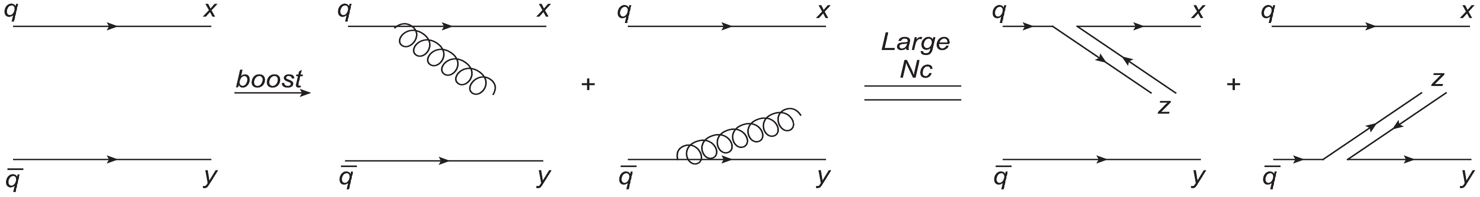
Figure 1. (color online) A schematic diagram of dipole rapidity evolution in the large
$ N_c $ limit. -
In this subsection, we perform a detailed derivation of the solution to the LO BK equation to introduce the method used to analytically solve the integral-differential equation. Here, we only consider the solution to the BK equation in the saturation domain because the physics of the dilute region is described by BKFL dynamics, which is relatively old. In the saturation region
$ r^2Q_s^2\gg1 $ , high energy dipole-hadron scattering approaches the black disk limit; thus, the scattering matrix$ S\rightarrow0 $ . Therefore, the non-linear term in S in Eq. (1) can be neglected, resulting in$ \begin{equation} \frac{\partial S(r, Y)}{\partial Y} \simeq -\frac{\bar{\alpha}_s}{2\pi}\int_{1/Q_s}^{r} \frac{ {{\rm{d}}}^2r_1 r^2}{r_1^2r_2^2} S(r, Y), \end{equation} $

(3) where
$ Q_s $ is the saturation scale. Note that we set the lower bound of the integral in Eq. (3) as$ 1/Q_s $ because the saturation condition demands that the transverse dipole size be greater than the typical dipole size$ r_s\sim1/Q_s $ . For the upper bound of the integral in Eq. (3), the parent dipole size r can be used. Although there are few emitted new dipoles with sizes larger than their parents$ r_1(r_2)>r $ , the evolution kernel$ K^{\mathrm{LO}} $ has a rapid decay when$ r_1(r_2)>r $ ; hence, the contribution from the$ r_1(r_2)>r $ region is negligible. The integral in Eq. (3) is governed by the situation in which either one of the daughter dipoles has a similar size to the parent dipole and the remaining one is significantly smaller than the parent dipole,$ r_2\sim r $ and$ r_1\ll r $ , or$ r_1\sim r $ and$ r_2\ll r $ [31,34]. Therefore, a factor of 2 is included on the right hand side of Eq. (4). If working in the first region, Eq. (3) reduces to$ \begin{equation} \frac{\partial S(r, Y)}{\partial Y} \simeq -2\frac{ \bar{\alpha}_s}{2}\int_{1/Q_s^2}^{r^2} \frac{ {{\rm{d}}} r_1^2}{r_1^2} S(r, Y). \end{equation} $

(4) Now, we perform integration over
$ r_1 $ and Y in Eq. (4) and obtain the analytic solution to the LO BK equation as [34,35]$ \begin{equation} S(r, Y) = \exp\left[-\frac{\lambda \bar{\alpha}_s^2}{2}(Y-Y_0)^2\right]S(r, Y_0), \end{equation} $

(5) where we use
$ \begin{equation} Q_s^2(Y) = \exp\big[\lambda \bar{\alpha}_s(Y-Y_0)^2\big]Q_s^2(Y_0) \end{equation} $

(6) and
$ \begin{equation} Q_s^2(Y_0)r^2 = 1. \end{equation} $

(7) Eq. (5) is known as the Levin-Tuchin formula [35]. We would like to emphasize that Eq. (5) is derived under the condition of fixed running coupling, which means that
$ \alpha_s $ is a constant and does not depend on parent dipole size or the smallest dipole size among the parent and two daughters (r,$ r_1 $ ,$ r_2 $ ). Thus, Eq. (5) is a leading order solution. The exponent of the S-matrix has a quadratic rapidity dependence, which makes the S-matrix too small when Y is large. In terms of the relationship between the S-matrix and scattering amplitude N,$ N = 1-S $ , the rapidity evolution speed of the scattering amplitude is too fast. It is for this reason that the LO BK equation is incapable of providing a precise description of the experimental data at HERA [13,14,36-38]. In the next section, we shall see that the argument of running coupling has a significant impact on the solution of the BK equation. As a consequence, the quadratic rapidity dependence in the exponent of the S-matrix shall convert into linear rapidity dependence once the running coupling effect is considered. -
From Sec.II, we know that the LO BK equation only considers the resummation of leading logarithmic
$ \alpha_s\ln(1/x) $ corrections in the fixed coupling case. The scattering amplitude resulting from the LO BK equation is not supported by HERA data. Therefore, we must go beyond leading order accuracy to improve the predictive power of the CGC theory. -
The first attempt toward NLO corrections of the BK equation were performed by Balitsky in Ref. [20] and Kovchegov and Weigert in Ref. [21]. They resummed the
$ \alpha_sN_f $ contributions to all orders independently. In the language of Feynman diagrams, they considered the quark loop contributions. -
The rcBK equation can be written as
$ \begin{equation} \frac{\partial S(r, Y)}{\partial Y} = \int\, {{\rm{d}}}^2 r_1 \,K^{\mathrm{rc}}(r, r_1, r_2) \left[S(r_1, Y)\,S(r_2, Y)-S(r, Y)\right], \end{equation} $

(8) where the evolution kernel
$ K^{\mathrm{rc}}(r, r_1, r_2) $ has two prescriptions: the Balitsky type [20]$ \begin{aligned}[b] K^{\mathrm{rcBal}}(r, r_1, r_2) =& \frac{N_c\alpha_s(r_{\mathrm{min}}^2)}{2\pi^2}\left[\frac{r^2}{r_1^2r_2^2} + \frac{1}{r_1^2}\left(\frac{\alpha_s(r_1^2)}{\alpha_s(r_2^2)}-1\right) \right.\\&\left.+ \frac{1}{r_2^2}\left(\frac{\alpha_s(r_2^2)}{\alpha_s(r_1^2)}-1\right)\right], \end{aligned} $

(9) and the Kovchegov-Weigert type [21]
$ \begin{aligned}[b] K^{\mathrm{rcKW}}(r, r_1, r_2) =& \frac{N_c}{2\pi^2}\left[\frac{\alpha_s(r_1^2)}{r_1^2}\right.\\&\left.-\frac{2\alpha_s(r_1^2)\alpha_s(r_2^2)}{\alpha_s(R^2)}\frac{{\boldsymbol{r_1}}\cdot{\boldsymbol{r_2}}}{r_1^2r_2^2}+\frac{\alpha_s(r_2^2)}{r_2^2}\right], \end{aligned} $

(10) with
$ \begin{equation} R^2(r, r_1, r_2) = r_1r_2\left(\frac{r_2}{r_1}\right)^{\textstyle\frac{r_1^2+r_2^2}{r_1^2-r_2^2}-\frac{2}{r_1^2-r_2^2}\frac{r_1^2r_2^2}{{\boldsymbol{r}_1\cdot{\boldsymbol{r}}_2}}}. \end{equation} $

(11) Note that the evolution kernels in Eq. (9) and Eq. (10) appear to differ at first glance because two types of separation schemes were used to isolate running coupling from subtraction in Refs. [20,21] (for the details on the separation schemes, see [22]). Interestingly, in our previous study, we found that both evolution kernels in the saturation region reduce to [31,33]
$ \begin{equation} K^{\mathrm{rc}}(r, r_1, r_2)\simeq\frac{N_c}{2\pi^2}\frac{\alpha_s(r_{\mathrm{min}}^2)}{r_1^2}. \end{equation} $

(12) From Eqs. (9) and (10), it is clear that the evolution kernel is modified by the running coupling corrections, which slows down the rapidity evolution speed of the scattering amplitude. As a consequence, the rcBK equation (8) greatly improve the predictive power of the CGC theory. The rcBK equation is more favored by HERA data than the LO BK equation [13]. Note that we will not provide a detailed derivation of the rcBK equation because it is outside the scope of this paper. In this study, we focus on the impact of running coupling on the evolution speed of the scattering amplitude. To reveal the effect of running coupling, we must analytically and numerically solve the rcBK equation. In the subsequent sections, it shall be revealed that the running coupling effect plays a significant role in dragging down the evolution of the CGC system.
-
To solve the rcBK equation (8), the format of the QCD coupling
$ \alpha_s $ must be identified. In this work, we plan to use the QCD coupling at one loop accuracy$ \begin{equation} \alpha_s(r^2) = \frac{1}{b\ln\Bigg(\dfrac{1}{r^2\Lambda^2}\Bigg)}, \end{equation} $

(13) with
$ b = (11N_c-2N_f)/12\pi $ .As with the LO BK equation, we analytically solve the rcBK equation in the saturation domain, which means that the sizes of the parent dipole (r) and two daughter dipoles (
$ r_1 $ and$ r_2 $ ) are larger than$ 1/Q_s $ . Therefore, we know that the lower and upper bounds of the integral in Eq. (8) are$ 1/Q_s $ and r, respectively. In addition, in the saturation domain, the integral in Eq. (8) is dominated by the case if one of the daughters has a similar size to the parent dipole while the remaining daughter is significantly smaller than the parent dipole. Using the approximation in Eq. (12) and assuming that$ r_1 $ is the smallest among the three dipoles, Eq. (8) can be simplified to$ \begin{aligned}[b] \frac{\partial S(r, Y)}{\partial Y} \simeq& \frac{N_c}{2\pi^2} 2 \int_{1/Q_s}^r\ \frac{ {{\rm{d}}}^2 r_1\alpha_s(r_1^2)}{r_1^2} \\&\times \left[S(r_1, Y)\,S(r_2, Y)-S(r, Y)\right]. \end{aligned} $

(14) Note that there is a symmetric factor of 2 on the right hand side of Eq. (14) owing to the fact that the larger or smaller dipole can be either of the emitted daughter dipoles. More importantly, in Eq. (14), the QCD coupling
$ \alpha_s $ has an argument$ r_1 $ in the running coupling case, which is not a constant as in the fixed coupling case. We choose to use the smallest dipole size running coupling prescription, which was proposed in Ref. [23] and developed by Ref. [25] and our previous publication [33]. In the smallest running coupling prescription, the argument of the running coupling is$ r_1 $ in Eq. (14). In the saturation region, the scattering amplitude tends toward 1; hence, the S-matrix is close to 0 as$ S\rightarrow0 $ . The quadratic term in S in Eq. (14) can be neglected and has the following approximation:$ \begin{equation} \frac{\partial S(r,Y)}{\partial Y}\simeq -\int_{1/Q_s^2}^{r^2}\, \,\frac{ {{\rm{d}}} r_1^2\bar{\alpha}_s(r_1^2)}{r_1^2}S(r, Y), \end{equation} $

(15) $ \begin{equation} S(r,Y) = \exp\left\{-\frac{N_c}{b\pi}(Y-Y_0)\left[\ln\left(\frac{\sqrt{\lambda'(Y-Y_0)}}{\ln\frac{1}{r^2\Lambda^2}}\right)-\frac{1}{2}\right]\right\}S(r, Y_0). \end{equation} $

(16) Here, we use
$ \ln Q_s^2/{\Lambda'}^2 = \sqrt{\lambda'(Y-Y_0)} + \mathcal{O}(Y^{1/6}) $ with$ \Lambda' $ fixed by the initial condition [39]. Let us compare the solution of the rcBK equation (16) with the solution to the LO BK equation (5). It is clear that the quadratic rapidity dependence in the exponent of the S-matrix changes to a linear dependence once the running coupling effect is considered, which dramatically suppresses the evolution speed of the scattering amplitude. It has been shown in Ref. [13] that this suppression is favored by HERA data. -
It is known that the rcBK equation only includes quark loop corrections. Soon after its formation, the full NLO BK equation was derived including gluon loop corrections in addition to quark loop corrections in Ref. [23]. However, the full NLO BK equation was found to be unstable owing to large double transverse logarithmic contributions in the evolution kernel,
$ -\ln r_1^2/r^2\ln r_2^2/r^2 $ [40]. To remove these instabilities, kinematical constraint [24] and resummation [25] methods were independently proposed. They obtained two stabilized full NLO BK equations, which were equivalent to each other in terms of the resummation of the leading double transverse logarithms and are known as the collinearly-improved BK equation. -
The ciBK equation can be written as [25]
$ \begin{equation} \frac{\partial S(r, Y)}{\partial Y} \simeq \frac{1}{2\pi}\int {\rm d}^2r_1K^{\mathrm{ci}}[S(r_1, Y)S(r_2, Y) - S(r, Y)], \end{equation} $

(17) where the collinearly-improved kernel is [41]
$ \begin{aligned}[b] K^{\mathrm{ci}} = & K^{\mathrm{DLA}}\Bigg[\frac{r^2}{r_1^2r_2^2} + \frac{1}{r_1^2}\Bigg(\frac{\alpha_s(r_1^2)}{\alpha_s(r_2^2)}-1\Bigg)+\frac{1}{r_2^2}\Bigg(\frac{\alpha_s(r_2^2)}{\alpha_s(r_1^2)}-1\Bigg)\Bigg] \\ & +\frac{ \bar{\alpha}_s(r^2)r^2}{r_1^2r_2^2}\Bigg(\frac{67}{36} - \frac{\pi^2}{12} - \frac{5N_f}{18N_c}\Bigg), \end{aligned} $

(18) with the double logarithmic approximation (DLA) evolution kernel
$ \begin{equation} K^{\mathrm{DLA}} = \frac{J_1\bigg(2\sqrt{ \bar{\alpha}_s \rho^2}\bigg)}{\sqrt{ \bar{\alpha}_s\rho^2}}\simeq 1 - \frac{ \bar{\alpha}_s\rho^2}{2} + \mathcal{O}( \bar{\alpha}_s^2). \end{equation} $

(19) $ J_1 $ in Eq. (19) is the Bessel function with the definition$ \begin{equation} \rho = \sqrt{\ln\frac{r_1^2}{r^2}\ln\frac{r_2^2}{r^2}}. \end{equation} $

(20) In addition, note that if
$ \begin{equation} \ln\frac{r_1^2}{r^2}\ln\frac{r_2^2}{r^2} < 0, \end{equation} $

(21) an absolute value is used and the Bessel function converts from
$ J_1 $ to$ I_1 $ [42]$ \begin{equation} K^{\mathrm{DLA}} = \frac{I_1\bigg(2\sqrt{ \bar{\alpha}_s \rho^2}\bigg)}{\sqrt{ \bar{\alpha}_s\rho^2}}. \end{equation} $

(22) Now, it is clear that the ciBK equation (17) is stable because the large double transverse logarithmic term disappeared from the evolution kernel of the ciBK equation (see Eq. (18)). From Eq. (18), we know that there is a DLA contribution, which is a result of double transverse logarithmic resummation.
-
Let us now analytically solve the ciBK equation. We will work in the saturation domain, where the ciBK equation is governed by the case of one of the two daughter dipoles having a similar size to the parent dipole while the remaining daughter is smaller than the parent dipole. In this case, the DLA kernel can simplify to
$ \begin{equation} K^{\mathrm{DLA}}\simeq 1 - \frac{ \bar{\alpha}_s\rho^2}{2}\simeq 1, \; \; \; \; \; \; \; \mathrm{when}\; \; r_1\sim r\; \; \mathrm{or}\; \; r_2\sim r. \end{equation} $

(23) Then, the ciBK evolution kernel reduces to
$ \begin{equation} K^{\mathrm{ci}}({\boldsymbol{r}},{\boldsymbol{r}}_1,{\boldsymbol{r}}_2) \simeq \frac{ \bar{\alpha}_s(r_{\min}^2)}{2\pi r_1^2} + \frac{ \bar{\alpha}_s^2(r_{\min}^2)}{8\pi r_1^2}\left(\frac{67}{9} - \frac{\pi^2}{3} - \frac{10N_f}{9N_c}\right). \end{equation} $

(24) Here, we once again note that the smallest dipole running coupling prescription is employed. Substituting Eq. (24) into Eq. (17) and performing integration over rapidity and dipole size, we can obtain an analytic solution to the ciBK equation.
$ \begin{aligned}[b] S(r, Y) =& \exp\Bigg\{-\frac{N_c}{b\pi}(Y-Y_0)\bigg[\ln\bigg(\frac{\sqrt{\lambda'(Y-Y_0)}}{\ln\frac{1}{r^2\Lambda^2}}\bigg)+\\& \frac{B'N_c}{b\pi\ln\frac{1}{r^2\Lambda^2}}-\frac{1}{2}\bigg] +\frac{2B'N_c^2}{b^2\lambda'\pi^2}\sqrt{\lambda'(Y-Y_0)}\Bigg\}S(r,Y_0), \end{aligned} $

(25) with
$ B' = 67/36-\pi^2/12-5N_f/18N_c $ . By comparing the analytic solution to the ciBK equation (25) with the solution to the rcBK equation (16), we can see that the dominant parts in the exponent of the S-matrices are similar; both have linear rapidity dependence under the smallest dipole running coupling prescription. This outcome indicates that the running coupling effect plays a major role in the suppression of the evolution speed of the scattering amplitude, especially in the saturation domain. In other words, although the resummation effect plays a significant role in removing instability from the NLO BK equation, it is not a dominant effect in the suppression of dipole evolution. -
Until now, all of the evolution equations mentioned above have been represented by the projectile rapidity Y. Recently, it was found that the instability issue in the full NLO BK equation is caused by the wrong choice of evolution variable, which means that the evolution variable in the BK equation should not be the projectile rapidity. From previous handling of similar unstable issues in the NLO BFKL equation, it is known that the proper evolution variable in the NLO BK equation ought to be the target rapidity η. By using the change of variable method,
$ Y = \eta+\rho $ , the authors in Ref. [26] derived a semi collinearly-improved Balitsky-Kovchegov equation in a target rapidity (ciBK-η) representation. The reason why we call it the semi ciBK-η equation is that it does not include full running coupling corrections. In our recent study [29], we developed upon the semi ciBK-η equation by including running coupling corrections during the expansion of the "real'' S-matrix and obtained an extended collinearly-improved BK equation in the target rapidity (exBK-η) representation. -
To obtain the ciBK-η equation, we must briefly introduce the full NLO BK equation in the Y-representation, which can be written as [20]
$ \begin{aligned}[b] \frac{\partial S(r, Y)}{\partial Y} =& \frac{ \bar{\alpha}_s}{2 \pi} \int {{\rm{d}}}^2 r_1\,\cdot (K_0 + K_q + K_g) \\&\cdot \Big(S(r_1, Y) S(r_2, Y) - S(r, Y) \Big) \\& +\frac{ \bar{\alpha}_s^2}{8\pi^2} \int {{\rm{d}}}^2 r_1 \, {{\rm{d}}}^2 r_2'\cdot K_1 \\ & \cdot \Big(S(r_1, Y) S(r_3, Y) S(r_2', Y) - S(r_1, Y) S(r_2, Y)\Big) \\& + \frac{ \bar{\alpha}_s^2}{8\pi^2}\frac{N_f}{N_c}\int {{\rm{d}}}^2 r_1 \, {{\rm{d}}}^2 r_2' \\&\times K_f\cdot\Big(S(r_1', Y)S(r_2, Y)-S(r_1, Y) S(r_2, Y)\Big), \end{aligned} $

(26) with
$ \begin{align} K_0 = \frac{r^2}{r_1^2r_2^2}, \end{align} $

(27) $ \begin{align} K_{q} = \frac{r^2}{r_1^2r_2^2} \bar{\alpha}_s \left[b \ln r^2 \mu^2 - b\frac{r_1^2 - r_2^2}{r^2} \ln\frac{r_1^2}{r_2^2} \right], \end{align} $

(28) $ \begin{align} K_{g} & = \frac{r^2}{r_1^2r_2^2} \bar{\alpha}_s\bigg[ \frac{67}{36} - \frac{\pi^2}{12} -\frac{5N_f}{18N_c} -\frac{1}{2}\ln \frac{r_1^2}{r^2} \ln \frac{r_2^2}{r^2}\bigg], \end{align} $

(29) $ \begin{aligned}[b] K_1 =& -\frac{2}{r_3^4} + \Bigg[\frac{r_1^2r_2'^2 + r_1'^2r_2^2 - 4r^2r_3^2}{r_3^4(r_1^2r_2'^2-r_1'^2r_2^2)}\\& + \frac{r^4}{r_1^2r_2'^2(r_1^2r_2'^2 - r_1'^2r_2^2)} + \frac{r^2}{r_1^2r_2'^2r_3^2}\Bigg]\ln\frac{r_1^2r_2'^2}{r_1'^2r_2^2}, \end{aligned} $

(30) and
$ \begin{align} K_f = \frac{2}{r_3^4} - \frac{r_1'^2r_2^2 + r_2'^2r_1^2 - r^2r_3^2}{r_3^4(r_1^2r_2'^2 - r_1'^2r_2^2)}\ln\frac{r_1^2r_2'^2}{r_1'^2r_2^2}, \end{align} $

(31) where
$ r_1'^2 = ({\boldsymbol{x}}-{\boldsymbol{u}})^2 $ ,$ r_2'^2 = ({\boldsymbol{y}}-{\boldsymbol{u}})^2 $ ,$ r_3^2 = ({\boldsymbol{z}}-{\boldsymbol{u}})^2 $ , and the kernels$ K_q $ and$ K_g $ denote the NLO corrections from the quark loop and gluon contributions. In the large$ N_c $ limit, Eq. (26) has a probability interpretation: the parent dipole ($ {\boldsymbol{x}}, {\boldsymbol{y}} $ ) splits into two daughter dipoles ($ {\boldsymbol{x}}, {\boldsymbol{z}} $ ) and ($ {\boldsymbol{z}}, {\boldsymbol{y}} $ ) with a common transverse coordinate$ {\boldsymbol{z}} $ . Then, the dipole ($ {\boldsymbol{z}}, {\boldsymbol{y}} $ ) further splits into dipoles ($ {\boldsymbol{u}}, {\boldsymbol{z}} $ ) and ($ {\boldsymbol{u}}, {\boldsymbol{y}} $ ) with a common transverse coordinate$ {\boldsymbol{u}} $ .Now, we transform Eq. (26) from the Y-representation to the η-representation using a change of variable
$ \begin{equation} Y = \eta + \rho. \end{equation} $

(32) Therefore, the S-matrices can be expressed in the η representation as
$ \begin{align} S(r, Y) = S(r, \eta+\rho) \equiv \bar{S}(r, \eta), \end{align} $

(33) $ \begin{aligned}[b] S(r_1, Y) =& S(r_1, \eta+\rho) = \bar{S}\left(r_1, \eta +\ln\frac{r_1^2}{r^2}\right)\\\simeq&\bar{S}(r_1, \eta) + \ln\frac{r_1^2}{r^2} \frac{\partial \bar{S}(r_1, \eta)}{\partial \eta}, \end{aligned} $

(34) $ \begin{aligned}[b] S(r_2, Y) =& S(r_2, \eta+\rho) = \bar{S}\left(r_2, \eta +\ln\frac{r_2^2}{r^2}\right)\\\simeq&\bar{S}(r_2, \eta) + \ln\frac{r_2^2}{r^2} \frac{\partial \bar{S}(r_2, \eta)}{\partial \eta} \end{aligned} $

(35) with
$ \rho = \ln Q^2/Q_0^2 $ .Substituting Eqs. (33), (34), and (35) into Eq. (26), and after some complex algebra, the ciBK-η equation can be obtained as [26]
$ \begin{aligned}[b] \frac{\partial S(r_1, \eta)}{\partial \eta} =& \, \frac{ \bar{\alpha}_s}{2 \pi} \int {{\rm{d}}}^2 r_1\cdot K_0\cdot\, \Theta\big(\eta - \delta_{r;r_1;r_2}\big) \\&\times\Big(\bar{S}(r_1, \eta - \delta_{r_1;r})\bar{S}(r_2, \eta - \delta_{r_2;r}) - \bar{S}(r, \eta) \Big) \\ & +\frac{ \bar{\alpha}_s}{2 \pi}\int {{\rm{d}}}^2 r_1 \cdot (K_q + K_g)\, \Big(\bar{S}(r_1, \eta) \bar{S}(r_2, \eta) - \bar{S}(r, \eta) \Big) \\ & +\frac{ \bar{\alpha}_s^2}{8\pi^2} \int {{\rm{d}}}^2 r_1\, {{\rm{d}}}^2 r_2'\, \cdot (K_1 + 4K_2) \\ &\cdot \Big(\bar{S}(r_1, Y) \bar{S}(r_3, Y) \bar{S}(r_2', Y) - \bar{S}(r_1, Y) \bar{S}(r_2, Y)\Big) \\ & + \frac{ \bar{\alpha}_s^2}{8\pi^2}\frac{N_f}{N_c}\int {{\rm{d}}}^2 r_1 \, {{\rm{d}}}^2 r_2' \cdot K_f\\&\cdot \Big(\bar{S}(r_1', Y)\bar{S}(r_2, Y)-\bar{S}(r_1, Y) \bar{S}(r_2, Y)\Big), \end{aligned} $

(36) with
$ K_2 = r^2/(r_1'^2r_3^2r_2^2)\ln r_2'^2/r^2 + \delta_{r_2';r} $ ,$\delta_{r_2';r} = \max\{0, \ln r^2/r_2'^2\}$ ,$ \delta_{r_1;r} = \max\{0,\ln r^2/r_1^2\} $ , and$ \delta_{r_2; r} = $ $ \max\{0,\ln r^2/r_2^2\} $ . If only the dominant part is retained, the canonical form of the BK equation (caBK-η) can be obtained as [26]$ \begin{aligned}[b] \frac{ \partial \bar{S}(r, \eta)}{ \partial \eta} =& \frac{ \bar{\alpha}_s}{2\pi} \int {{\rm{d}}}^2 r_1 \cdot K_0\cdot\, \Theta\big(\eta - \delta_{r;r_1;r_2}\big) \\ &\times\big[\bar{S}(r_1, \eta - \delta_{r_1;r})\bar{S}(r_2, \eta - \delta_{r_2;r}) - \bar{S}(r, \eta) \big], \end{aligned} $

(37) which is a non-local evolution equation in rapidity η. The rapidity shifts in Eq. (37) act as resummation.
The ciBK-η equation only includes part of the running coupling corrections; it does not include the running coupling contributions of the Taylor expansions in (34), and (35). To obtain a full running coupling improved ciBK-η equation, we re-derive it by considering all running coupling corrections in the Taylor expansions (see [29] for a detailed derivation). From this, we obtain the running coupling improved ciBK-η equation [29]
$ \begin{aligned}[b] \frac{\partial S(r_1, \eta)}{\partial \eta} =& \, \frac{ \bar{\alpha}_s}{2 \pi} \int {{\rm{d}}}^2 r_1\cdot K_0\cdot\, \Theta\big(\eta - \delta_{r;r_1;r_2}\big) \\&\times\Big(\bar{S}(r_1, \eta - \delta_{r_1;r})\bar{S}(r_2, \eta - \delta_{r_2;r}) - \bar{S}(r, \eta) \Big) \\ & +\frac{ \bar{\alpha}_s}{2 \pi}\int {{\rm{d}}}^2 r_1 \cdot (K_q + K_g)\, \Big(\bar{S}(r_1, \eta) \bar{S}(r_2, \eta) - \bar{S}(r, \eta) \Big) \\ & +\frac{ \bar{\alpha}_s^2}{8\pi^2} \int {{\rm{d}}}^2 r_1\, {{\rm{d}}}^2 r_2'\, \cdot (K_1 + 4K_3) \\&\cdot \Big(\bar{S}(r_1, Y) \bar{S}(r_3, Y) \bar{S}(r_2', Y) - \bar{S}(r_1, Y) \bar{S}(r_2, Y)\Big) \\ & + \frac{ \bar{\alpha}_s^2}{8\pi^2}\frac{N_f}{N_c}\int {{\rm{d}}}^2 r_1 \, {{\rm{d}}}^2 r_2' \cdot K_f\\&\cdot \Big(\bar{S}(r_1', Y)\bar{S}(r_2, Y)-\bar{S}(r_1, Y) \bar{S}(r_2, Y)\Big), \end{aligned} $

(38) with
$ \begin{aligned}[b] K_3 =& \bigg(\ln\frac{r_2'^2}{r^2}+\delta_{r_2';r}\bigg)\bigg[ \frac{r^2}{r_1'^2\,r_3^2\,r_2^2}+ \frac{r^2}{r_1'^2\,r_2'^2}\frac{1}{r_3^2}\left(\frac{ \alpha_s^{r_3}}{ \alpha_s^{r_2}}-1\right) \\ &+ \frac{r^2}{r_1'^2\,r_2'^2r_2^2}\left(\frac{ \alpha_s^{r_2}}{ \alpha_s^{r_3}}-1\right)+ \frac{r_2'^2 }{r_1'^2r_3^2\,r_2^2}\left(\frac{ \alpha_s^{r_1'}}{ \alpha_s^{r_2'}}-1\right) \\ &+ \frac{1}{r_1'^2r_3^2}\left(\frac{ \alpha_s^{r_1'}}{ \alpha_s^{r_2'}}-1\right)\left(\frac{ \alpha_s^{r_3}}{ \alpha_s^{r_2}}-1\right)+ \frac{1}{r_1'^2r_2^2}\left(\frac{ \alpha_s^{r_1'}}{ \alpha_s^{r_2'}}-1\right)\left(\frac{ \alpha_s^{r_2}}{ \alpha_s^{r_3}}-1\right) \\ &+ \frac{1}{r_3^2\,r_2^2}\left(\frac{ \alpha_s^{r_2'}}{ \alpha_s^{r_1'}}-1\right)+ \frac{1}{r_2'^2r_3^2}\left(\frac{ \alpha_s^{r_2'}}{ \alpha_s^{r_1'}}-1\right)\left(\frac{ \alpha_s^{r_3}}{ \alpha_s^{r_2}}-1\right) \\ &+ \frac{1}{r_2'^2r_2^2}\left(\frac{ \alpha_s^{r_2'}}{ \alpha_s^{r_1'}}-1\right)\left(\frac{ \alpha_s^{r_2}}{ \alpha_s^{r_3}}-1\right) \bigg], \end{aligned} $

(39) where we use variations of the shorthand notation
$ \alpha_s^{r_1} = \alpha_s(r_1^2) $ for all terms. Similar to Eq. (37), if only the dominant part is retained, the extended BK equation in target rapidity representation (exBK-η) can be obtained as [29]$ \begin{aligned}[b] \frac{ \partial \bar{S}(r, \eta)}{ \partial \eta} =& \int {{\rm{d}}}^2 r_1 K_{\mathrm{rc}}(r,r_1,r_2) \Theta\big(\eta - \delta_{r;r_1;r_2}\big) \\&\times\big[\bar{S}(r_1, \eta - \delta_{r_1;r})\bar{S}(r_2, \eta - \delta_{r_2;r}) - \bar{S}(r, \eta) \big], \end{aligned} $

(40) which has the same structure as the caBK-η equation (37), but with a running coupling modified kernel
$ K_{\mathrm{rc}} = \bar{\alpha}_s(K_0+K_q)/2\pi $ . -
To intuitively understand the significance of the running coupling effect, we shall analytically solve the caBK-η and exBK-η equations in the saturation region for the fixed and running coupling cases, respectively. We employ the same strategy we used for the solutions to the LO BK and rcBK equations. We are interested in the saturation domain where one of the two daughter dipoles is much smaller than the other, while the large daughter is close to the parent dipole. In this section, we also assume
$ 1/Q_s\ll r_1\ll r_2 $ and$ r_2\sim r $ . It is known that the non-locality (or rapidity shift) is only important for the S-matrix associated with the smaller dipole. Therefore, the impact of the rapidity shift can be neglected for the larger dipole. Eq. (37) reduces to$ \begin{aligned}[b] \frac{ \partial\bar{S}(r,\eta)}{ \partial\eta} \simeq &\frac{ \bar{\alpha}_s\bar{S}(r,\eta)}{\pi}\int_{1/Q_s}^{r}\frac{ {{\rm{d}}}^2r_1}{r_1^2}\Theta\bigg(\eta-\ln\frac{r^2}{r_1^2}\bigg) \\&\times\left[\bar{S}\bigg(r_1,\eta-\ln\frac{r^2}{r_1^2}\bigg)-1\right], \end{aligned} $

(41) where
$ Q_s $ is the saturation momentum, which is associated with$ \bar{Q}_s $ via$ r^2Q_s^2 = (r^2\bar{Q}_s^2)^{1/(1+\bar{\lambda})} $ [26].Now, we solve Eq. (41) in the saturation domain, where the scattering amplitude approaches 1 and thus the S-matrix is close to 0. This indicates that the S-matrix in the square brackets on the right hand side of Eq. (41) can be neglected because it is much smaller than 1. Thus, Eq. (41) simplifies to
$ \begin{equation} \frac{ \partial\bar{S}(r,\eta)}{ \partial\eta} \simeq - \bar{\alpha}_s\bar{S}(r,\eta)\int_{1/Q_s^2}^{r^2}\frac{ {{\rm{d}}} r_1^2}{r_1^2}. \end{equation} $

(42) Performing integration over
$ r_1 $ and η, we can obtain the analytic solution to the caBK-η equation in the saturation domain as$ \begin{equation} \bar{S}(r,\eta) = \exp\left[-\frac{ \bar{\alpha}_s^2}{2}\frac{\bar{\lambda}\big(\eta - \eta_0\big)^2}{1+ \bar{\alpha}_s\bar{\lambda}}\right]\bar{S}(r,\eta_0), \end{equation} $

(43) where
$ \begin{equation} \bar{Q}_s^2 = Q_0^2\exp(\bar{\lambda}\eta). \end{equation} $

(44) From Eq. (42), we can see that the QCD coupling
$ \alpha_s $ is fixed. We will not artificially represent$ \alpha_s $ as a function of the size of the smallest dipole because running coupling was not included when deriving the caBK-η equation. In the fixed coupling case, the S-matrix has a quadratic rapidity dependence in its exponent (43), which is similar to the solution of the LO BK equation (5), although the coefficients in the exponent are slightly different. The quadratic rapidity dependence implies a rapid evolution speed in the scattering amplitude, which is not favored by the proton structure data at HERA.Next, we solve the running coupling modified exBK-η equation, Eq. (40), in the saturation domain. From solving the rcBK equation in Sec. III.A, we know that the evolution kernel
$ K_{\mathrm{rc}} $ in Eq. (40) can reduce to$ K^{\mathrm{rc}} $ , Eq. (12). Furthermore, the non-locality is only important for the S-matrix associated with the smaller dipole. Thus, we can obtain a simplified Eq. (40) as follows:$ \begin{aligned}[b] \frac{ \partial \bar{S}(r,\eta)}{ \partial \eta} \simeq& \frac{\bar{S}(r,\eta)}{\pi}\int_{1/Q_s}^{r} \frac{ {{\rm{d}}}^2r_1}{r_1^2} \bar{\alpha}_s(r_1^2) \Theta\Big(\eta - \ln\frac{r^2}{r_1^2}\Big)\\&\times \left[\bar{S}\Big(r_1, \eta - \ln\frac{r^2}{r_1^2}\Big) - 1\right]. \end{aligned} $

(45) At first glance, it seems that Eq. (45) is almost the same as Eq. (41). However, there is a key difference caused by QCD running coupling.
$ \alpha_s $ is fixed in Eq. (41), whereas$ \alpha_s $ is a function of the size of the smallest dipole among the parent and daughter dipoles in Eq. (45). It is precisely because of$ \alpha_s $ that the rapidity dependences of the scattering amplitude greatly differs.In the saturation domain, it is known that the S-matrix is close to 0. The S-matrix in square brackets on the right hand side of Eq. (45) is negligible. Using one loop running coupling, Eq. (13), we can obtain a simplified Eq. (45) as
$ \begin{align} \frac{ \partial \bar{S}(r,\eta)}{ \partial \eta} \simeq -\frac{N_c\bar{S}(r,\eta)}{\pi}\int_{1/Q_s^2}^{r^2} \frac{ {{\rm{d}}} r_1^2}{r_1^2}\frac{1}{b\ln\dfrac{1}{r_1^2\Lambda^2}}, \end{align} $

(46) whose solution is
$ \begin{aligned}[b] \bar{S}(r,\eta) =\exp \Bigg\{-\frac{N_c}{b\pi}(\eta - \eta_0) \end{aligned} $

$ \begin{aligned}[b]\quad\quad\times \left[\ln \left(\dfrac{\sqrt{\bar{\lambda'}}(\eta-\eta_0)+\dfrac{\sqrt{\bar{\lambda'}}}{2}\ln\dfrac{1}{r^2\Lambda^2}}{\left(\sqrt{\eta-\eta_0}+\dfrac{\sqrt{\bar{\lambda}'}}{2} \right)\ln\dfrac{1}{r^2\Lambda^2}} \right)-\dfrac{1}{2} \right] \Bigg\}\bar{S}(r,\eta_0), \end{aligned} $

(47) where
$ \ln\bar{Q}_s^2/{\Lambda'}^2 = \sqrt{\bar{\lambda}'(\eta-\eta_0)} + \mathcal{O}(\eta^{1/6}) $ and$ r^2Q_s^2 \simeq \left[r^2\bar{Q}_s^2 \right]^{1/(1+\sqrt{\bar{\lambda}'/4\eta})} $ .So far, we have obtained five analytic solutions, Eqs. (5), (16), (25), (43), and (47) for five different BK evolution equations, Eqs. (1), (8), (17), (37), and (40), respectively. Now, two comparisons are performed: (i) the two solutions with the fixed QCD coupling, (5) and (43), have a quadratic rapidity dependence, which leads to rapid evolution speeds in the scattering amplitude; (ii) the three solutions with running QCD coupling, (16), (25), and (47), have similarly linear rapidity dependences, which yield a favored HERA data scattering amplitude. This outcome indicates that running coupling plays a significant role in the precise description of experimental data. Interestingly, we observe that the running coupling corrections cause the rapidity dependence in the exponent of the S-matrix to change from quadratic to linear dependence regardless of whether the evolution equations are equipped in the projectile rapidity (Y) or target rapidity (η) representation. This suggests that the running coupling corrections overwhelm the contribution from the changing of evolution variable. Finally, it is clear why the ciBK, kcBK, and exBK-η equations used in Ref. [30] provide indistinguishable descriptions of the reduced cross section data at HERA, because these three equations yield similar scattering amplitudes in the running coupling case.
-
In this section, we numerically solve the BK equations to test the analytic results obtained in previous sections. It is known that the BK equations are integro-differential equations that can be solved via the Runge-Kutta method. We shall use the GNU Scientific Library (GSL) to perform the numerical analysis, since the GSL provides almost all of the numerical routines required by our purpose. In this study, we do not consider the impact parameter dependence and assume that the dipole amplitude is independent of angle,
$N({\boldsymbol{r}}, Y) = $ $ 1-S({\boldsymbol{r}}, Y) = $ $ 1-S(|r|, Y)$ .For the initial condition of the BK equations, we use the McLerran-Venugopalan (MV) model to parameterize the scattering amplitude at rapidity
$ Y = 0 $ [43]$ \begin{equation} S^{\mathrm{MV}}(r, Y = 0) = \exp\bigg[-\bigg(\frac{r^2Q_{s0}^2}{4}\bigg)^{\gamma}\ln\Big(\frac{1}{r^2\Lambda^2}+e\Big)\bigg], \end{equation} $

(48) where
$ Q_{s0}^2 $ and γ are the free parameters that shall be determined by fitting to HERA data.For
$ \alpha_s $ in the BK equations, we use the one-loop QCD coupling constant, Eq. (13), with$ N_f = 3 $ and$ N_c = 3 $ . The smallest dipole running coupling prescription is employed in these numerical simulations.$ \begin{equation} \alpha_s(r_{\mathrm{min}}^2) = \alpha_s\big(\mathrm{min}\{r^2,r_1^2,r_2^2\}\big). \end{equation} $

(49) Running coupling
$ \alpha_s(r_{\mathrm{fr}}) = 0.75 $ is frozen when$ r>r_{\mathrm{fr}} $ to regularize the infrared behavior. -
The left-hand panel of Fig. 2 presents the solutions to the LO BK and rcBK equations for three different rapidities. Note that we only select two typical groups of solutions to the BK equations to unambiguously reveal the role of the running coupling effect. The dashed and solid curves denote the results computed by the LO BK and rcBK equations, respectively. In addition, the blue, red, and purple curves present numerical solutions at rapidities of 4, 8, and 12, respectively. The black curve is the MV initial condition. By comparing the solutions for each respective rapidity, we can see that the values of the scattering amplitudes resulting from the rcBK equation are significantly smaller than those from the LO BK equation, which implies that the running coupling corrections significantly slow down the evolution speed of the scattering amplitude. This outcome is consistent with the analytic solution obtained in Sec. III.A, in which the running coupling effect converts the quadratic rapidity dependence in the LO case (5) into linear rapidity dependence in the NLO case (16); as a consequence, the evolution speed of the scattering amplitude is suppressed by the running coupling effect.
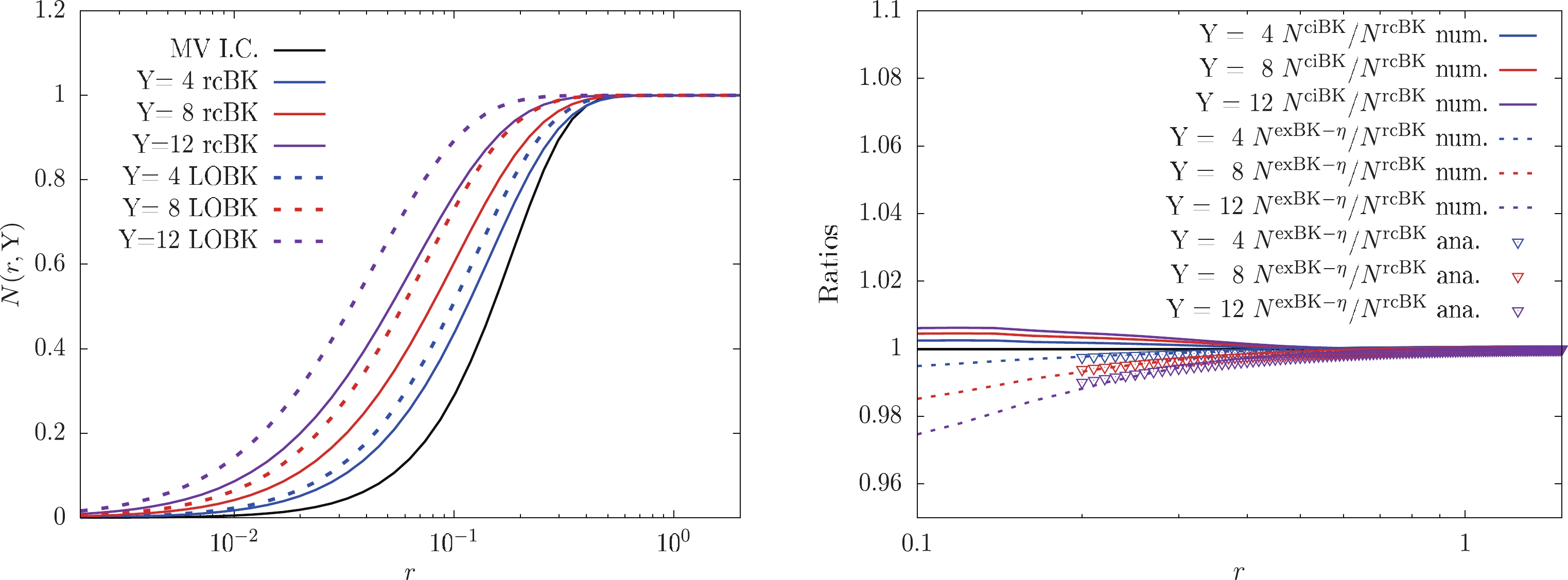
Figure 2. (color online) Numerical solutions to the BK equations for three different rapidities. The left hand panel presents comparisons of the evolution speeds of the LO scattering amplitude and running coupling modified scattering amplitude. The right hand panel shows the respective ratios of the ciBK and exBK-η equation solutions to the rcBK equation solutions.
The right-hand panel of Fig. 2 shows the ratios of the ciBK, and exBK-η equation solutions to the rcBK equation solutions in the saturation domain for rapidities of 0 (black curve), 4 (blue curves), 8 (red curves), and 12 (purple curves). The solid and dashed curves denote the ratios
$ N^{\mathrm{ciBK}}/N^{\mathrm{rcBK}} $ and$ N^{\mathrm{exBK-\eta}}/N^{\mathrm{rcBK}} $ computed from the exact numerical solutions to these equations. By comparing the ratios for each respective rapidity, we can see that all ratios are close to one, which indicates that the scattering amplitudes resulting from the rcBK, ciBK, and exBK-η equations are similar in the saturation domain. The numerical results support the analytic findings in Sec. III.C.2. These numerical results can provide a reasonable explanation as to why the kcBK, ciBK, and exBK-η equations provide equally high quality descriptions of HERA data in Ref. [30]. Moreover, to compare the numerical and analytic solutions, the ratio$ N^{\mathrm{exBK-\eta}}/N^{\mathrm{rcBK}} $ (triangles) computed by the analytic expressions is plotted in Fig. 2. Note that Fig. 2 only shows the analytic ratios in relatively large dipole sizes because the analytic amplitudes are valid only in the saturation region, for example,$ rQ_s>2 $ [9]. The analytic ratios are consistent with the numerical ratios. -
To further support the outcomes obtained above, we use the rcBK (8), ciBK (17), and exBK-η (40) equations to fit HERA data [44]. The actual quantity we shall fit is the reduced cross-section
$ \begin{equation} \sigma_\mathrm{red} = \frac{Q^2}{4\pi^2\alpha_{\mathrm{em}}}\bigg[\sigma_{\mathrm{T}}^{\gamma^\ast p}+\frac{2(1-y)}{1+(1-y)^2}\sigma_{\mathrm{L}}^{\gamma^\ast p}\bigg], \end{equation} $

(50) with
$ y = Q^2/(sx) $ as the inelasticity variable and s the squared center of mass collision energy.$ \sigma_{\mathrm{T}} $ and$ \sigma_{\mathrm{L}} $ in Eq. (50) are the transverse and longitudinal cross-sections, respectively.$ \begin{equation} \sigma_{\mathrm{T,L}}^{\gamma^\ast p} = \sum_f\int_0^1{\rm d}z\int {\rm d}^2r|\psi^{(f)}_\mathrm{T,L}(r,z;Q^2)|^2\sigma_\mathrm{dip}^{q\bar{q}}(r,x), \end{equation} $

(51) where
$ \psi^{(f)}_\mathrm{T,L} $ is the light cone wave function, which can be calculated via QED [45]. The key term in Eq. (51) is the dipole amplitude$ \sigma_\mathrm{dip}^{q\bar{q}} $ , which can be expressed in terms of the S-matrix,$ \sigma_\mathrm{dip}^{q\bar{q}}(r, x) = \sigma_0 \big[1- S(r, x)\big] $ . Here,$ \sigma_0 $ denotes the area of the proton and is a free parameter in our fit. To obtain a good description of HERA data, it is useful to slightly modify the one loop running coupling Eq. (13) to$ \alpha_s(r^2) = 1/[b\ln(4C/r^2\Lambda^2)] $ with C as a free parameter.Within the framework of the color glass condensate, we must work in a small x region,
$ x<0.01 $ . Thus, there are 252 data points from Ref. [44] being used in our fit. Table 1 provides the values of the relevant parameters. Reasonable$ \chi^{2}/\mathrm{d.o.f} $ values indicate that BK equations with higher order corrections provide good description of HERA data. In particular, note that$ \chi^{2}/\mathrm{d.o.f} $ resulting from the three higher order BK (rcBK, ciBK, and exBK-η) equations have similar values, which suggests that they provide HERA data descriptions of similar quality.Dipole amplitude $ \sigma_0 $ /mb

$\bar{Q}_{s0}^2/\mathrm{GeV}^2$ 

γ $ C^2 $ 

$ \chi^{2}/\mathrm{d.o.f} $ 

rcBK 30.75 0.16 1.10 5.20 1.15 ciBK 31.51 0.15 1.05 26.56 1.26 exBK-η 33.24 0.13 1.08 0.80 1.20 Table 1. Parameters and
$ \chi^{2}/\mathrm{d.o.f} $ from the fits.To intuitively display the good matching between the theoretical calculations and experimental data, we plot the reduced cross-section versus x for different values of
$ Q^2 $ in Fig. 3. The green squares, red circles, and blue triangles denote the numerical results computed using the rcBK, ciBK, and exBK-η equations, respectively. From Fig. 3, we can see that almost all of the numerical results overlap with the data points, which indicates once again that the three aforementioned BK equations provide similar descriptions of HERA data. Because the rcBK equation (with only running coupling corrections) is relatively low among the three higher order equations, we can reason that the NLO BK equation running coupling correction is only sufficient in the description of the experimental data at HERA energies.
Figure 3. (color online) The reduced cross-section as a function of x at different values of
$ Q^2 $ . The experimental data points are from the combined measurements of the H1 and ZEUS collaborations [44]. -
In this paper, we first presented analytic solutions to the LO BK, rcBK, ciBK, and exBK-η equations in the saturation region for the fixed and running coupling cases. By comparing these equations, we found that all of the analytic S-matrices in the final three (NLO) equations had similar linear rapidity dependence in the exponent, which indicates that the running coupling correction was the main correction among all NLO corrections (for example, gluon loop and collinear resummation) in the suppression of the rapidity evolution of the dipole amplitude. Thus, the dominant part of the dipole amplitudes resulting from the final three equations was almost the same (see Eqs. (16), (25), and (47)). This finding can provide a reasonable explanation for a surprising result presented in Ref. [30], where the authors found that different fit schemes (kcBK, ciBK, and exBK-η) resulted in equally good descriptions of HERA data. Our study found that the running coupling BK equation was robust and had a sufficiently strong predictive power for the DIS measurements at HERA energies, although other higher order corrections may be significant for future experiments, such as those at the EIC or LHeC.
To test the analytic outcomes mentioned above, we numerically solved the BK equations and calculated the ratios between these solutions (see Fig. 2). The ratios were close to one in the saturation region, which suggests that the three dipole amplitudes were almost equal and confirmed our analytic findings. Moreover, we numerically fit the three dipole amplitudes to HERA data. The
$ \chi^2/\mathrm{d.o.f} $ obtained from the fits reveals that the three equations provide an equally good description of HERA data (see also Fig. 3). In short, our study suggests that the BK equation with NLO correction at the running coupling level has sufficient accuracy to describe HERA data.
Running coupling effect in next-to-leading order Balitsky-Kovchegov evolution equations
- Received Date: 2021-10-11
- Available Online: 2022-05-15
Abstract: Balitsky-Kovchegov equations in projectile and target rapidity representations are analytically solved for fixed and running coupling cases in the saturation domain. Interestingly, we find that the respective analytic S-matrices in the two rapidity representations have almost the same rapidity dependence in the exponent in the running coupling case, which provides a method to explain why the equally good fits to HERA data were obtained when using three different Balitsky-Kovchegov equations formulated in the two representations. To test the analytic outcomes, we solve the Balitsky-Kovchegov equations and numerically compute the ratios between these dipole amplitudes in the saturation region. The ratios are close to one, which confirms the analytic results. Moreover, the running coupling, collinearly-improved, and extended full collinearly-improved Balitsky-Kovchegov equations are used to fit the HERA data. We find that all of them provide high quality descriptions of the data, and the


 DownLoad: