


 Abstract
 HTML
HTML Reference
 Related
 PDF
PDF


-
Experimental datasets for the pion vector form factor have important applications in elementary particle physics, notably providing input for a high precision determination of the muon anomalous magnetic moments, which is one of the prospective probes for a "new physics" discovery [1]. The quantity in the limit of low energy can be related to the pion charge radius, an observable that describes the quantum chromodynamics (QCD) confinement of the pion. An accurate determination of the radius provides a precision test in the realm of the standard model of particle physics at low energy (e.g., chiral perturbation theory and lattice QCD) [2]. The analyses of high quality data for the pion form factor also yield a straightforward computation of the pion charge radius, particularly through dispersion theory approaches [2-4], and it is principally cited in the Particle Data Group (PDG) booklet [5]. The PDG 2020 has published the following updated value:
$\sqrt{\langle r_{V}^{2} \rangle} = $ $ (0.659 \pm 0.004)\;{\rm{ fm}}$ .In this study, we focus on analyzing the experimental datasets for the modulus of the pion vector form factor to extract the value of the pion charge radius within a Bayesian framework. The datasets were obtained from the measurements of
$ e^{+}e^{-}\rightarrow \pi^{+}\pi^{-} $ experiments [6-11]. The phenomenological fit used in our work is an approach from the dispersion theory of the electromagnetic structure of hadrons described in [3]. Theoretically, the pion form factor formulated using this approach utilizes a holomorphic function, colloquially called a "polynomial," whose corresponding polynomial order terms are constrained specifically from the data fitting. The rapid progress in high performance computing, as well as advanced numerical algorithms dedicated to Bayesian analysis, has created interest toward Bayesian tools for analyzing and inferring data in hadron physics [12]. Henceforth, our problems can be solved using model selection techniques that can be conducted via the Bayesian approach.In addition to computing the Bayesian evidences, we performed model comparisons based on Bayesian effective complexity to determine the effective number of model parameters sufficient for describing the datasets. Despite the non-universal definition of effective model complexity in the Bayesian framework [13], this work employed a formalism of model selection in terms of a trade-off between a goodness-of-fit and model complexity proposed in the context of physical sciences and widely used in cosmology and astrophysics in particular [14-18]. The complexity attempts to break degeneracy among the competing models (two or more models having the same magnitude of Bayesian evidences) using Occam's razor to penalize the large volume of the "unused" parameter space of the more complex model(s) [15].
-
We specify
$ p({{\theta}} \lvert {\bf{y}},{\cal{M}}) $ as the probability that a model denoted by$ {\cal{M}} $ with a set of parameters$ {{\theta}} = \left\{ \theta_{1}, \theta_{2}, ..., \theta_{m} \right\} $ is true, given a dataset$ {\bf{y}} $ that has k data points$ {\bf{y}} = \left\{ y_{1}, y_{2}, ..., y_{k} \right\} $ with any background information incorporated in$ {\cal{M}} $ . This quantity is called a posterior, representing the updated probability of the model parameters after we observe the given dataset,$ {\bf{y}} $ . We express Bayes' theorem as [19]$ p({{\theta}} \lvert {\bf{y}},{\cal{M}}) = \frac{{\cal{L}}({\bf{y}}\lvert {{\theta}}, {\cal{M}}) \pi({{\theta}} \lvert {\cal{M}})}{p({\bf{y}}\lvert {\cal{M}})} . $

(1) The quantity
$ {\cal{L}}({\bf{y}}\lvert {{\theta}}, {\cal{M}}) $ is the$ likelihood $ , which expresses the probability of observing the dataset$ {\bf{y}} $ if the model$ {\cal{M}} $ is true. The quantity$ \pi({{\theta}} \lvert {\cal{M}}) $ is the$ prior\; probability $ , which accommodates our prior knowledge of the model parameters before observing the data. The quantity in the denominator,$ p({\bf{y}}\lvert {\cal{M}}) $ , is called the$ evidence $ , which serves as a normalization factor and is given by the integral over the parameter space.The Bayesian model selection aims to directly compare the relative probability of two competing models fitted to the data. Hence, we define the Bayes factor, namely, the ratio of evidences between two competing models
$ {\cal{M}}_{1} $ and$ {\cal{M}}_{2} $ , as$ B_{12} \equiv \frac{p({\bf{y}} \lvert {\cal{M}}_{1})}{p({\bf{y}} \lvert {\cal{M}}_{2})}. $

(2) The Bayes factor describes whether the data permits a sensible selection of a model if the order of magnitude of the model evidence significantly exceeds the evidence of other competing models.
Generally, a simple model that can provide a satisfactory description of the data is more favored than more complex models (i.e., models with many parameters), which is the essence of Occam's razor. Thus, we employ
$ Bayesian \;effective $ $ \;complexity $ , denoted as$ {\cal{C}}_{b} $ , which measures the effective number of model parameters that the data can support [15, 17, 20]. The quantity is defined in terms of the Kullback-Leibler divergence between the posterior and prior. However, assuming that the likelihood function of our model can be expressed as$ {\cal{L}}(\theta) = \exp{(-\chi^{2}(\theta)/2)} $ ,$ {\cal{C}}_{b} $ can be expressed in a compact form [16, 17]:$ {\cal{C}}_{b} = \overline{\chi^{2}(\theta)}-\chi^{2}(\widehat{\theta}). $

(3) where
$ \overline{\chi^{2}(\theta)} $ is determined over the posterior distribution,$ \overline{\chi^{2}(\theta)} = \int p(\theta \lvert {\bf{y}}, {\cal{M}})\,\chi^{2}(\theta) \,{\rm{d}}\theta. $

(4) The second term is a point-estimate of the likelihood function around the estimator of the parameters,
$ \hat{\theta} $ . The estimator is selected to be any of the sample statistics that best represents the posterior distribution.In principal, the Bayesian effective complexity provides a tool to overcome degeneracy in the value of the model evidences between two or more models. For example, if we consider two models,
$ {\cal{M}}_{1} $ and$ {\cal{M}}_{2} $ , with the number of model parameters$ m_{1}<m_{2} $ , then the following scenario can be used to asses the models:(i)
$ {\cal{C}}_{b}({\cal{M}}_{2}) \geqslant {\cal{C}}_{b}({\cal{M}}_{1}) $ and$ p({\bf{y}}\lvert{\cal{M}}_{2}) \gg p({\bf{y}}\lvert{\cal{M}}_{1}) $ : the most complex model$ ({\cal{M}}_{2}) $ is favored, implying that the extra parameters are permitted by the data.(ii)
$ p({\bf{y}}\lvert{\cal{M}}_{2}) \approx p({\bf{y}}\lvert{\cal{M}}_{1}) $ and$ {\cal{C}}_{b}({\cal{M}}_{2})>{\cal{C}}_{b}({\cal{M}}_{1}) $ : the quality of the data does not significantly improve the evidence of the more complex model; hence, Occam's razor demands the selection of a model with fewer parameters.(iii)
$ p({\bf{y}}\lvert{\cal{M}}_{2}) \approx p({\bf{y}}\lvert{\cal{M}}_{1}) $ and$ {\cal{C}}_{b}({\cal{M}}_{2}) \approx {\cal{C}}_{b}({\cal{M}}_{1}) $ : the data may not be sufficient to permit the additional parameters, and we are unable to make any conclusive decision as to whether the additional parameters are required, unless$ {\cal{C}}_{b}({\cal{M}}_{2})<m_{2}. $ The parameter estimation and model selection based on
$ {\cal{C}}_{b} $ can be performed using Markov chain Monte Carlo (MCMC) algorithms to provide an efficient sampling of analytically intractable posterior distributions① [21]. We employ an affine – invariant ensemble sampling introduced by Goodman et al., [22] and the improved implementation by Foreman-Mackey et al. [23] is available as a package called$ {\texttt{EMCEE}} $ . In this study, we used$ {\texttt{EMCEE}} $ to provide the sampling of the posterior distribution.Following the suggestion in [23], we initialized the algorithm by beginning a set of walkers to explore a small Gaussian ball in the parameter space around a certain point (i.e., a set of initial values of the parameters with a maximum likelihood probability). The walkers diffused to the surrounding parameter space to eventually explore the full posterior distribution. We initially ran a chain with hundreds to thousands of samples, which was determined via trial and error for each scenario, to achieve a "burn-in" phase. Thereafter, the desired posterior distribution was computed by generating
$ O(10^{5}) $ samples. -
Below the inelastic threshold, namely energy less than 1.0 GeV2, we can employ Watson's theorem [24] to parameterize the pion vector form factor expressed as a product of two functions:
$ F_{V}(s) = P(s)\Omega(s), $

(5) where
$ P(s) $ is an arbitrary holomorphic function, and$ \Omega(s) $ is called Omnès function [25], defined as$ \Omega(s) = \exp \left\{ \frac{s}{\pi} \int_{4m_{\pi}^{2}}^{\infty} \frac{{\rm{d}}z}{z} \frac{\delta_{1}(z)}{z-s-{\rm i}\epsilon} \right\}. $

(6) Equation (5) is known as the Omnès representation of the pion form factor with the input of
$ \pi\pi $ P-wave phase shifts.Meanwhile, the holomorphic function,
$ P(s) $ , can be expressed as a polynomial whose degree depends on the high energy continuation and the final state interactions. Moreover, we consider the$ \rho-\omega $ mixing effect to explain the narrow structure in the$ \rho-\omega $ mass region of the$ e^{+}e^{-}\rightarrow\pi\pi $ data. We follow an ansatz proposed in [3] that assumes form as a simple Breit-Wigner parameterization of the$ \omega $ -channel into the polynomial$ P(s) $ . Thus, the final form of the polynomial up to the third order can be expressed as$ P(s) = (1+\alpha s +\beta s^{2} + \gamma s^{3})+ \frac{\kappa_{1} s}{m_{\omega}^{2}- s -i m_{\omega}\Gamma_{\omega}}. $

(7) Here,
$ m_{\omega} $ and$ \Gamma_{\omega} $ are the$ \omega $ -mass and its total decay width, respectively. A new parameter$ \kappa_{1} $ is obtained via a fit to the data for the pion form factor. We can exclude higher order terms when we are assured that a lower order polynomial can still explain the observed data.The squared charge radius of the pion,
$ \langle r_{V}^{2} \rangle $ , is associated with the first derivative of the pion form factor evaluated at$ s = 0 $ :$ \langle r_{V}^{2} \rangle \equiv 6 \frac{{\rm d}F_{V}(s)}{{\rm{d}}s}\Bigr\rvert_{s = 0}. $

(8) Using Eqs. (5) and (6),
$ \langle r_{V}^{2} \rangle $ can be expressed in terms of the polynomial and Madrid parameters:$ \langle r_{V}^{2} \rangle = \frac{6}{\pi}\int_{4m_{\pi}^{2}}^{\infty} \frac{\delta_{1}(z)}{z^{2}}\,{\rm{d}}z + 6\left( \alpha + \frac{\kappa_{1}}{m_{\omega}^{2}} \right). $

(9) Throughout this work, the phase shift,
$ \delta_{1} $ , used in Eq. (6) was obtained from the phenomenological fits to the$ \pi\pi $ data provided in [26] known as$ Constrained $ $ \;Fits \;to \;Data $ (CFD) set (we refer to this formulation as Madrid phase shift) in an energy range up to$ 1.42 $ GeV. The parameterization of the phase shift is summarized in Table 1 including their pertinent (symmetric) uncertainties. The continuation of the phase shift above$ 1.42 $ GeV is possible using any smooth extrapolation that fulfills the asymptotic condition$ \delta_{1}(s)\rightarrow\pi $ . Therefore, we propose the following high-energy extension with an exponential decay factor:Parameter Value $ m_\rho $ 

$ 773.69 \pm 0.90 $ MeV

$ B_{0} $ 

$ 1.043 \pm 0.011 $ 

$ B_{1} $ 

$ 0.19 \pm 0.05 $ 

$ \lambda_{1} $ 

$ 1.39 \pm 0.18 $ 

$ \lambda_{2} $ 

$ 1.70 \pm 0.49 $ 

Table 1. Fit parameters of the P-wave phase shift obtained from the dispersive analysis of the Madrid group [26].
$ \begin{aligned}[b] c(s) =& \pi - \left[ (\pi-b(s_{m})) - (s-s_{m})b'(s_{m}) \right]\\&\times \exp\left(-\frac{(s-s_{m})^{2}}{T^{2}}\right)\Theta(s-s_{m}). \end{aligned} $

(10) Here,
$ b'(s_{m}) $ is the first derivative of the Madrid phase shift evaluated at the matching point,$ \sqrt{s_{m}}\leqslant $ 1.42 GeV (i.e., the boundary between the intermediate-energy and high-energy region). The other parameter (T) is a rate of decay of the above extension that eventually converges to$ \pi $ as the energy increases. Its value should be selected to maintain a continuous matching between the two energy regions. To achieve the aforementioned property, we select$ s_{m}\approx 1.3^{2} $ GeV2 and$ T\approx 2.0 $ GeV2. We might be able to consider the inclusion of the two parameters as a possible source of systematic uncertainty in the$ \langle r_{V}^{2} \rangle $ values. We refer to the Madrid phase shift with this type of high energy continuation as phase shift$ N\rho $ ,$ \delta_{1}^{N\rho}(s) $ .The formulation of the Omnès function in Eq. (6) and hence the pion form factor in Eq. (5) only hold for purely elastic interactions up to infinite energies (i.e., the phase shift
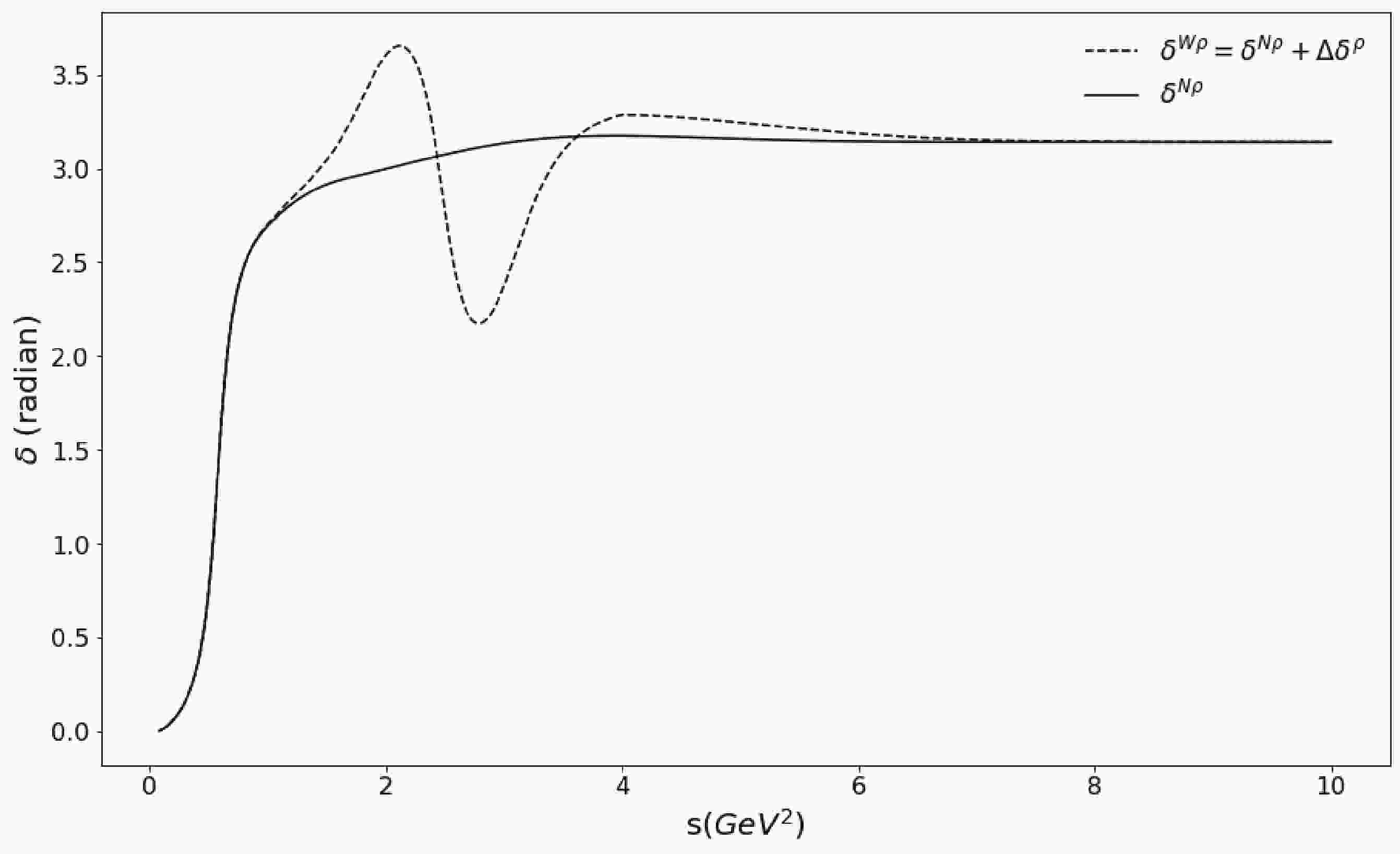
$ N\rho $ ). Physically, the inelasticity of the$ \pi\pi $ scattering for the P-wave is indicated by the experimental observations that indicate that, except for the existence of$ \rho $ resonance (or more precisely the$ \rho(770) $ meson and the$ \rho-\omega $ mixing) below (1.42${\rm GeV})^{2}$ , the line shape of$ F_{V} $ at higher energies contains structures such as the$ \rho-\phi $ mixing and other$ \rho $ resonances such as$ \rho(1450) $ and$ \rho(1770) $ (experimentally denoted as$ \rho' $ and$ \rho'' $ , respectively). To incorporate the effects of these higher$ \rho $ resonances, we employ a parameterization of the pion vector form factor introduced in [27]. Subsequently, we extract a phase shift difference, denoted by$ \Delta\delta(s) $ , that contains information about those high energy structures. The values can be added into the original phase shift$ N\rho $ ,$ \delta_{1}^{N\rho} $ to obtain phase shift$ W\rho $ , formulated as$ \delta_{1}^{W\rho}(s) \equiv \delta_{1}^{N\rho}+\Delta\delta(s) $ (Fig. 1). The phase shift is the second input to Eq. (5), which can be useful in providing a comparative result with the computation via the phase shift$ N\rho $ .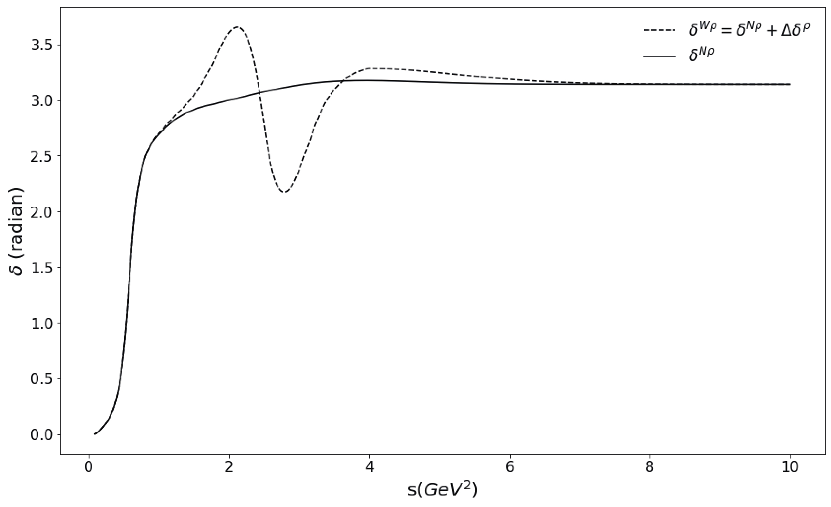
Figure 1. Comparison of two different
$\pi\pi$ scattering phase shifts ($\delta^{W\rho}$ and$\delta^{N\rho}$ ) with respect to energy s. -
We employed data from six different
$ e^{+}e^{-}\rightarrow\pi^{+}\pi^{-} $ experiments at timelike energies: KLOE10, KLOE12, BESIII, BABAR, CMD2, and SND [6-11]. More precisely, we only used the pion vector form factor that included vacuum polarization effects. First, KLOE10, KLOE12, BESIII, and BABAR events were divided into energy intervals (bins) with specific widths,$ \Delta $ . The number of data points and bin width included in our analysis were 75 points and$ \Delta = 10 $ MeV for KLOE10, 60 points and$ \Delta = 10 $ MeV for KLOE12, 60 points and$ \Delta = 5 $ MeV for BESIII, and 270 points,$ \Delta = 10 $ MeV below 500 MeV, and$ \Delta = 2 $ MeV for$ 500\;{\rm{ MeV}}<\sqrt{s} \leqslant 1000 \;{\rm{ MeV}} $ for BaBar. Therefore, we must modify the expression of the pion form factor at each bin according to the following formula:$ \widetilde{F}_{V}(s_{i}) = \frac{1}{2\sqrt{s_{i}}\Delta} \int\limits_{(\sqrt{s_{i}}-\Delta/2)^{2}}^{(\sqrt{s_{i}}+\Delta/2)^{2}} F_{V}(s) \,{\rm{d}}s, $

(11) where
$ \widetilde{F}_{V}(s_{i}) $ is the average value of the form factor at i-th bin,$ s_{i} $ is the energy value at the bin center, and$ F_{V}(s) $ denotes the original formulation given in Eq. (5). In contrast, the CMD2 (29 points) and SND (45 points) datasets were not divided into bins [10, 11]. The CMD2 and SND data are the simplest among the six datasets because they have$ \widetilde{F}_{V}(s_{i}) = F_{V}(s_{i}) $ . -
We performed the parameter inference to extract the values of the pion charge radius,
$ \langle r_{V}^{2} \rangle $ , for a single dataset in two separate scenarios. Each scenario involved different types of phase shifts ($ N\rho $ and$ W\rho $ ) as the input to the Omnès function in Eq. (6). Next, we compared the formulation of the form factor under the two scenarios with varying options of the degree of the polynomial$ P(s) $ . Selecting$ \beta = \gamma \equiv 0 $ and a non-zero value of$ \alpha $ , we acquired a linear polynomial. Meanwhile, a quadratic polynomial was obtained by maintaining non-zero values of$ \alpha $ and$ \beta $ ; and the cubic polynomial permitted the three coefficients to be non-zero. Therefore, the number of considered scenarios in each dataset was six, three for each phase shift scenario. In addition to the values of$ \langle r_{V}^{2} \rangle $ ,$ \kappa_{1} $ ,$ \alpha $ ,$ \beta $ , and$ \gamma $ , other nuisance parameters were considered in our analysis:$ \omega $ mass ($ m_{\omega} $ ) and its total width ($ \Gamma_{\omega} $ ), both of which are parameters in the Breit-Wigner function in Eq. (7). Moreover, parameters in the Madrid phase shift (i.e., Table 1), denoted as$ \theta_{M} = (m_{\rho}{, }B_{0}{, }B_{1}{, }\lambda_{1}, \;{\rm{and}}\;\lambda_{2}) $ , were also considered to be the nuisance parameters.To maintain a low computational cost of the numerical calculation of the Omnès function within the Bayesian integration, we approximated the expression of the Madrid phase shift in Taylor series only to the first order about the quoted mean values of Madrid parameters
$ \overline{\theta}_{M}^{(i)} $ . We assumed that those parameters only sway around the mean values within the small parameter space volume (with a radius measured from their standard deviations). Thus, we obtained$ \left|\Omega(s,\theta_{M}^{(i)}) \right|^{2} \approx \lvert \Omega(s,\overline{\theta}_{M}^{(i)})\rvert^{2} \left| \exp\left( \frac{s}{\pi}(\theta_{M}^{(i)} - \overline{\theta}_{M}^{(i)}) \int {\rm d}z \frac{D^{(i)}(s)}{z(z-s)} \right) \right|^{2}, $

(12) where
$ D^{(i)}(s) $ denotes the partial derivative of the phase shift with respect to the parameter$ \theta_{M}^{(i)} $ .For simplicity, we further assumed that the experimental data were obtained from a Gaussian distribution (independent observations) with diagonal covariance matrices. The probability for the data
$ {\bf{y}}\equiv \lvert F_{V}^{2}\rvert $ , where each data point is denoted as$ y_{i} $ with the measurement error$ \sigma_{i} $ , to occur under the assumption of the pion form factor of Equation (5), i.e., the likelihood, is expressed as$\begin{aligned}[b] & \ln{\cal{L}}\left( {\bf{y}} \lvert \langle r_{V}^{2} \rangle, \alpha, \beta, \gamma, \kappa, m_{\omega}, \Gamma_{\omega}, \theta_{M} \right) \propto \\-&\frac{1}{2}\sum\limits_{k} \left( \frac{\lvert \widetilde{F}_{V}(s_{i},\langle r_{V}^{2} \rangle, \alpha, \beta, \gamma, \kappa, m_{\omega}, \Gamma_{\omega}, \theta_{M})\rvert^{2} - y_{i}}{\sigma_{i}} \right)^{2}. \end{aligned} $

(13) We propose a normal distribution,
$ {\cal{N}}(\overline{\theta}_{M},\sigma_{\theta_{M}}) $ , to express our prior beliefs of all parameters used in the Madrid phase shift whose central values are$ \overline{\theta}_{M} $ and errors are$ \sigma_{\theta_{M}} $ . More precisely, the total prior probability of all Madrid parameters,$ \pi(\theta_{M}) $ , can be expressed as$ \pi(\theta_{M}) \sim \prod\limits_{j = 1}^{5} {\cal{N}}(\overline{\theta}_{M,j},\sigma_{\theta_{M,j}}), $

(14) Moreover, we considered
$ m_{\omega} $ and$ \Gamma_{\omega} $ to be nuisance parameters and assume normal distributions with mean values and errors obtained from PDG [5]. We also employed a Gaussian prior for the pion charge radius, and its mean and uncertainty were also obtained from PDG 2020.On the contrary, it is rather unclear how to establish prior beliefs for
$ \kappa_{1} $ ,$ \beta $ , and$ \gamma $ . However, we argue that both "informative" and "uninformative" priors can still be used for$ \kappa_{1} $ ,$ \beta $ , and$ \gamma $ . To avoid cluttering the notation, we denote$ \pi_{A} $ and$ \pi_{B} $ as the informative and uninformative priors for the three parameters, respectively [28].● Informative priors,
$ \pi_{A} $ The fit values of
$ \kappa_{1} $ have been explored in [3] and [4]. Hanhart et al. provided an estimate of this quantity via the experimental value of the total decay width of$ \omega $ obtained from PDG. In this study, we used their formula to obtain$ \kappa_{1} = (1.99 \pm 0.36)\times 10^{-3} $ . Therefore, we set the prior for$ \kappa_{1} $ as$ {\cal{N}}(\overline{\kappa}_{1},\sigma_{\kappa_{1}}) $ based on that value. Meanwhile, we imposed a zero-mean Gaussian prior for$ \beta $ and$ \gamma $ and its variance was deduced from preliminary MCMC sampling. After several experimentations, we concluded that the width distribution for$ \gamma $ was relatively larger than$ \beta $ . Thus, we set the following prior for$ \gamma $ :$\pi_{\gamma}\approx {\cal{N}}(\mu = 0$ ${\rm{ GeV}}^{-6},\sigma = 0.5\;{\rm{ GeV}}^{-6})$ for the remainder of our analyses (i.e., using the same prior regardless of the data being used). In contrast, we propose the following priors for$ \beta $ : 1) the BABAR data uses$ \pi_{\beta}\approx {\cal{N}}(\mu = 0\;{\rm{ GeV}}^{-4},$ $\sigma = 0.2\;{\rm{ GeV}}^{-4}) $ , 2) the KLOE10 and KLOE12 data use$ \pi_{\beta}\approx{\cal{N}}(\mu = 0\;{\rm{ GeV}}^{-4} $ ,$\sigma = 0.3\;{\rm{ GeV}}^{-4}) $ , and 3) the CMD2, SND, and BESIII data use$ \pi_{\beta}\approx{\cal{N}}(\mu = 0\;{\rm{ GeV}}^{-4}, $ $ \sigma = 0.4\;{\rm{ GeV}}^{-4}) $ . The joint distribution for "informative" prior beliefs,$ \pi_{A} $ , is simply determined by the total product of the above priors:$ \pi_{A} = \pi(\theta_{M})\,\pi(m_{\omega},\Gamma_{\omega},\langle r_{V}^{2}\rangle)\,\,\pi_{A}(\kappa)\,\pi_{A}(\beta)\,\pi_{A}(\gamma). $

(15) ● Uninformative priors,
$ \pi_{B} $ To alleviate criticism over the selected prior and provide additional diagnosis of the results, we additionally assigned the
$ uninformative \;priors $ to the fit parameters. For the KLOE10, KLOE12, and BABAR datasets, we selected the priors for both$ \beta $ and$ \gamma $ to be flat within the ranges$ -1\;{\rm{ GeV}}^{-4} \leqslant \beta \leqslant 1\;{\rm{ GeV}}^{-4} $ and$ -1\;{\rm{ GeV}}^{-6} \leqslant \gamma \leqslant $ $ 1\;{\rm{ GeV}}^{-6} $ and then appended an exponential fallof beyond the given range:$ \pi(x) \sim \exp \left( \frac{\lvert x \rvert - 1 }{\lambda}\right). $

(16) Here
$ \lambda $ is set to$ 0.1\;{\rm{ GeV}}^{-4} $ for$ \beta $ and$ 0.5\;{\rm{ GeV}}^{-6} $ for$ \gamma $ , reflecting our vague understanding of parameter$ \gamma $ . We employed the same priors for CMD2, SND, and BESIII except that their range was selected from –2.0 units to 2.0 units because the preliminary MCMC computations demonstrated that their distributions are wider than the other datasets. Meanwhile, the fit values of$ \kappa_{1} $ are always observed to be in order$ \tau = 10^{-3} $ . Therefore, we may place the following exponential distribution as the prior for$ \kappa_{1} $ :$ \pi ({\kappa _1}) = \left\{ {\begin{array}{*{20}{l}} {\dfrac{1}{\tau }\exp \left( { - \dfrac{{{\kappa _1}}}{\tau }} \right),}&{{\rm{if}}\;{\kappa _1} > 0,}\\ {0,}&{{\rm{otherwise}}.} \end{array}} \right. $

(17) The joint prior,
$ \pi_{B} $ , is also determined by the total product of the individual priors.Owing to the strict relation in Equation 9, we can ignore
$ \alpha $ completely from our analysis and set the pion vector form factor as a function of$ \langle r_{V}^{2} \rangle $ instead of$ \alpha $ . Next, the posterior distribution can be formulated via Bayes' theorem (Equation 1) and computed via MCMC sampling. -
After the MCMC walker chains were established, we computed the estimate-measure of the marginalized distribution of
$ \langle r_{V}^{2} \rangle $ to obtain the radius value. In this paper, we opt to quote the "68.3% rule" used in [2] in the sense of a frequentist approach, stating that the percentage of the values within the band around the mean value defines a one-standard deviation,$ 1\sigma $ (Fig. 2). Normalizing the parameter distribution, we imposed the following condition: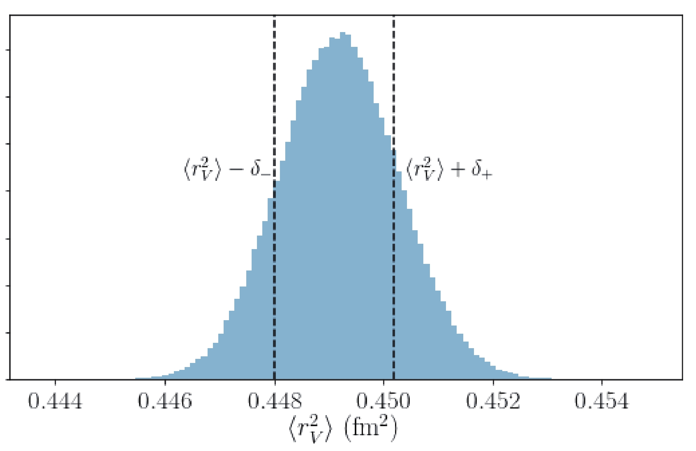
Figure 2. (color online) Marginal distribution of
$\langle r_{V}^{2} \rangle$ obtained via the A-W$\rho$ fit (i.e., applying the prior$\pi_{A}$ and including the higher$\rho$ resonances) using the BaBar data. The 68.3% confidence interval (CI) is marked by the two dashed lines.$ \int_{\overline{\theta}_{i}-\delta^-}^{\overline{\theta}_{i}+\delta^+}p(\theta_{i}\;\lvert {\bf{y}},{\cal{M}})\,\theta_{i}\,\;{\rm{d}}\theta_{i} = 68.3\%, $

(18) and solved it to obtain the upper and lower errors,
$ \delta_{+} $ and$ \delta_{-} $ .We established four different "fits" for our analyses based on the notation in the tables. The first fit A-W
$ \rho $ corresponded to the analysis using the informative priors ($ \pi_{A} $ ) for$ \kappa $ ,$ \beta $ , and$ \gamma $ as well as the phase shift$ \delta_{1}^{W\rho} $ ("with" higher$ \rho $ resonances). The fit A-N$ \rho $ employed the same prior$ \pi_{A} $ but used the phase shift$ \delta_{1}^{N\rho} $ ("no" higher$ \rho' $ resonances). The fit B-W$ \rho $ considered both the uninformative priors$ \pi_{B} $ and the$ \delta_{1}^{W\rho} $ . The final fit B-N$ \rho $ with the flat distributions excluded the resonances.We only show two prominent examples here: BaBar and BESIII analysis, presented in Table 2 and 3, since the conclusions from KLOE10, KLOE12, CMD, and SND were similar to that of BaBar, while the BESIII result provided an "outlier" compared with the others. The first column of each table provides the estimated values of the squared pion charge radius including their uncertainties, indicated in bracket(s). The symmetric error is shown as a number inside a single bracket. The values inside double brackets denote the upper and lower uncertainties (asymmetric errors), which clearly suggest a non-Gaussian nature of the marginal distribution of the parameters of interest.
Prior Resonance $ {\cal{M}} $ (

$ {\cal{C}}_{0} $ )

$ \langle r_{V}^{2}\rangle $ /fm2

$ \kappa\times 10^{-3} $ 

$ \beta $ /GeV

$ ^{-4} $ 

$ \gamma $ /GeV

$ ^{-6} $ 

$ p({\bf{y}}\lvert {\cal{M}}) $ 

$ {\cal{C}}_{b} $ 

$ \pi_{A} $ 

Fit A-W $ \rho $ 

L (9) 0.4491(11) 1.86(5) $ 0^{*} $ 

$ 0^{*} $ 

9.02 9.63 Q (10) 0.4446(26) 1.95(6)(6) 0.08(4) $ 0^{*} $ 

5.47 10.16 C (11) 0.4452(51) 1.95(7)(7) 0.07(7) 0.00(8) 1.00 10.32 Fit A-N $ \rho $ 

L (9) 0.4417(11) 1.89(5) $ 0^{*} $ 

$ 0^{*} $ 

21.44 9.33 Q (10) 0.4390(25) 1.94(6) 0.09(7) $ 0^{*} $ 

4.28 9.86 C (11) 0.4359(48) 1.92(7) 0.05(4) −0.05(6) 1.00 10.13 $ \pi_{B} $ 

Fit B-W $ \rho $ 

L (9) 0.4492(11) 1.86(5) $ 0^{*} $ 

$ 0^{*} $ 

54.46 9.48 Q (10) 0.4448(26) 1.95(6) 0.08(4) $ 0^{*} $ 

16.02 10.01 C (11) 0.4455(47) 1.95(7) 0.07(7) 0.00(8) 1.00 10.45 Fit B-N $ \rho $ 

L (9) 0.4418(11) 1.89(5) $ 0^{*} $ 

$ 0^{*} $ 

151.20 9.13 Q (10) 0.4391(24)(25) 1.93(6) 0.05(4) $ 0^{*} $ 

12.45 9.54 C (11) 0.4366(46)(45) 1.95(7) 0.07(7) 0.01(7) 1.00 10.83 Table 2. Bayesian analysis of the BaBar data employing four "fits", denoted by A-W
$ \rho $ , A-N$ \rho $ , B-W$ \rho $ , and B-N$ \rho $ as the combination of the prior and the phase shift.Prior Resonance $ {\cal{M}} $ (

$ {\cal{C}}_{0} $ )

$ \langle r_{V}^{2}\rangle $ /fm2

$ \kappa\times 10^{-3} $ 

$ \beta $ /GeV

$ ^{-4} $ 

$ \gamma $ /GeV

$ ^{-6} $ 

$ p({\bf{y}}\lvert {\cal{M}}) $ 

$ {\cal{C}}_{b} $ 

$ \pi_{A} $ 

Fit A-W $ \rho $ 

L (9) 0.4430(35)(33) 1.81(14) $ 0^{*} $ 

$ 0^{*} $ 

0.89 7.28 Q (10) 0.4232(93)(96) 1.81(15)(14) 0.18(8) $ 0^{*} $ 

1.82 8.09 C (11) 0.4050(216)(213) 1.87(15) 0.5(3) −0.2(3) 1.00 8.54 Fit A-N $ \rho $ 

L (9) 0.4328(31) 1.79(14) $ 0^{*} $ 

$ 0^{*} $ 

1.94 7.13 Q (10) 0.4185(91) 1.83(14) 0.13(8) $ 0^{*} $ 

1.11 7.98 C (11) 0.3976(219)(215) 1.84(14) 0.5(3) −0.3(3) 1.00 8.40 $ \pi_{B} $ 

Fit B-W $ \rho $ 

L (9) 0.4423(35)(33) 1.73(15) $ 0^{*} $ 

$ 0^{*} $ 

3.27 7.37 Q (10) 0.4230(95)(97) 1.79(16) 0.05(5)(4) $ 0^{*} $ 

1.13 7.92 C (11) 0.3577(371)(373) 1.80(16) 0.2(2) −0.1(1) 1.00 7.78 Fit B-N $ \rho $ 

L (9) 0.4321(34) 1.71(15) $ 0^{*} $ 

$ 0^{*} $ 

9.62 7.39 Q (10) 0.4148(94)(92) 1.76(15) 0.1(1) $ 0^{*} $ 

0.91 8.24 C (11) 0.3493(365)(371) 1.77(16) 1.2(6)(5) −0.9(5)(4) 1.00 8.13 Table 3. Bayesian analysis of the BESIII using fit A-W
$ \rho $ , A-N$ \rho $ , B-W$ \rho $ , and B-N$\rho$ .Our first observation was that when using
$ \delta_{1}^{W\rho} $ , the extracted radii for all considered polynomials were larger than that of$ \delta_{1}^{N\rho} $ . This indicated that a larger radius value may be caused by the net "positive" effect from the phase shift with$ \rho'-\rho'' $ phase. Moreover, it came as no surprise that the uncertainties increased as the degree of the polynomial increases because the extra prior coalescing into the existing posterior also further stretched the marginal distribution of the radius. Interestingly, the values of$ \kappa_{1} $ barely changed significantly in all fits referring to a single dataset, and the values were consistent with the results from [3, 4]. -
Model selection is performed by estimating the Bayes factor for
$ nested \;models $ , which means that we seek to compare a$ (m+1) $ -parameter model$ {\cal{M}}_{2} $ to a simpler m-parameter model$ {\cal{M}}_{1} $ , namely a submodel of$ {\cal{M}}_{2} $ when one parameter of$ {\cal{M}}_{2} $ is fixed. We denote the parameters of the complex model as$ \theta^{(2)} = (\psi,\theta^{(1)}) $ , where the simpler model$ {\cal{M}}_{1} $ is obtained by setting$ \psi = 0 $ . We further assume that the prior is also separable. Thus, we can prove that the Bayes factor$ B_{12} $ can be easily obtained here simply by computing the following ratio [15]:$ B_{12} = \frac{p(\psi \lvert {\bf{y}}, {\cal{M}}_{2})}{\pi(\psi \rvert {\cal{M}}_{2})}\bigg|_{\psi = 0}. $

(19) Here,
$ p(\psi \lvert {\bf{y}}, {\cal{M}}_{2}) $ is the marginal posterior of the more complex model while$ \pi(\psi \rvert {\cal{M}}_{2}) $ is the prior density of this more complex model. In Bayesian literature, this expression is known as the Savage-Dickey density ratio (SDDR) [16, 29, 30]. This method is suitable for our scenario, in which we only introduced one additional parameter into the original model to construct a more complex model, namely, from the linear model to the quadratic one or from the quadratic to the cubic one.The general prescription to calculate the value of the evidence of the three models begins from the marginal distribution of the cubic model parameter
$ p(\gamma \lvert {\cal{M}}_{\gamma}) $ obtained from the normalized MCMC sampling and normalized to unity. Practically, we can use a non-parametric method, such as$ Kernel \;Density \;Estimation $ , to investigate the distribution of a particular density plot to estimate the probability evaluated at the zero parameter value (i.e.,$ p(\gamma = 0 \lvert {\cal{M}}_{\gamma}) $ ). We pluged the result into Eq. (19), where the prior of$ \gamma $ was also computed at the zero parameter value,$ \pi(\gamma = 0 \lvert {\cal{M}}_{\gamma}) $ to obtain the Bayes factor between the quadratic model and the cubic one,$ B_{\beta\gamma} $ . The Bayes factor enabled us to calculate the model evidence using Eq. (2) as follows:$ p({\bf{y}} \lvert {{\cal{M}}_{\beta}}) = B_{\beta\gamma}\times p({\bf{y}} \lvert {{\cal{M}}_{\gamma}}), $

(20) where we assigned any arbitrary value to the cubic model evidence. For simplicity, we set
$ p({\bf{y}} \lvert {{\cal{M}}_{\gamma}})\equiv 1 $ , since we sought only to compare the relative magnitude of each model. We subsequently continued the same prescription to compute the evidence of the linear model$ p({\bf{y}} \lvert {{\cal{M}}_{\alpha}}) $ , beginning from the quadratic model. The final expression was similarly expressed as$ p({\bf{y}} \lvert {{\cal{M}}_{\alpha}}) = B_{\alpha\beta}\times B_{\beta\gamma}\times p({\bf{y}} \lvert {{\cal{M}}_{\gamma}}). $

(21) The origin of the difference in the values of the evidences obtained from the priors
$ \pi_{A} $ and$ \pi_{B} $ are shown in Tables 2 and 3, respectively. This can be explained more intuitively using the definition of the SDDR in Eq. (19). The informative distribution$ \pi_{A} $ was slightly peaked compared with the uninformative prior,$ \pi_{B} $ ; hence, the ratio between the marginal distribution and the prior in Eq. (19) was also directly affected.We depict the SDDR computation using the BaBar analysis for both
$ \beta $ and$ \gamma $ in Fig. 3. Here, the resulting marginal posteriors for the two choices of prior had almost similar positions (the height difference was also negligible), implying that the priors only moderately affected the posteriors. However, the height ratio between the posterior and the prior at the zero$ \beta $ or$ \gamma $ value (blue dashed lines) using$ \pi_{A} $ (black curve) was smaller than the ratio using$ \pi_{B} $ (red curve) because the Gaussian prior was slightly higher (i.e., more peaked) than the flat prior. If we further stretched the range of the parameter value in the flat prior$ \pi_{B} $ , the distribution height also decreased; hence, the ratio in Eq. (19) increased because the posterior was relatively stable against the selected prior. The same conclusion also held if we selected a larger variance for a Gaussian prior.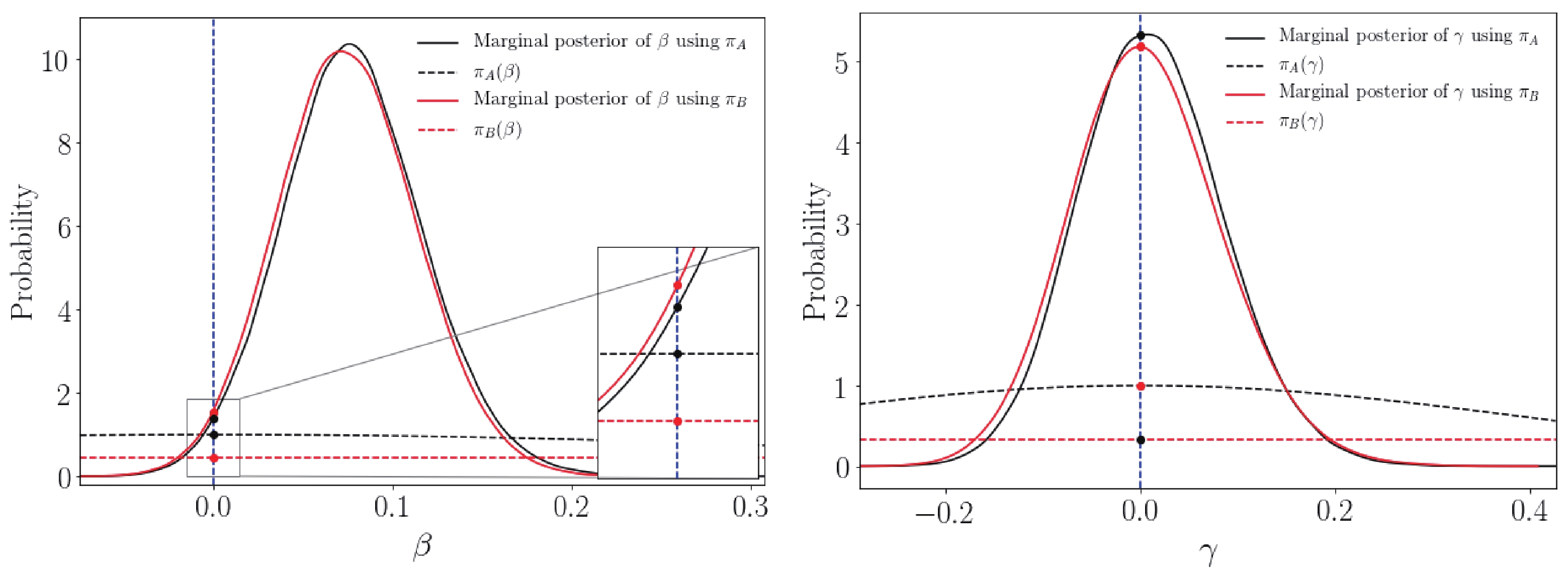
Figure 3. (color online) Marginal distributions of
$ \beta $ and$ \gamma $ in the BaBar analysis with$ \delta_{1}^{W\rho} $ . The results are compared using two different choices of priors. The height ratio between the marginal distribution and the prior evaluated at zero value (black and red dots on the blue line) illustrates the computation of the SDDR in Eq. (19). -
We required the efficient Bayesian complexity,
$ {\cal{C}}_{b} $ , to provide a means of inferring the number of free parameters the data could still constraint. The quantity is expressed by Eq. (3) where$ \chi^{2} $ and$ \hat{\theta} $ were approximated using a estimator describing the resulting MCMC chain. However, a good estimator for non-Gaussian posterior distributions is difficult to obtain and is consdiered to be the main problem in some references [17, 18]). Therefore, we utilized various estimators (i.e., maximum a posteriori, posterior mean, posterior median, and posterior mode) or combinations of those quantities to obtain sensible values of$ {\cal{C}}_{b} $ .We summarize the results in Figs. 4 and 5. The left-hand figures plot the
$ {\cal{C}}_{b} $ against the real number of parameters$ {\cal{C}}_{0} $ . The line$ {\cal{C}}_{b} = {\cal{C}}_{0} $ is an auxiliary to check the consistency between the obtained effective number of parameters ($ {\cal{C}}_{b} $ ) with$ {\cal{C}}_{0} $ . A good inference is indicated by the points that do not deviate significantly from the line until a certain critical point at which$ {\cal{C}}_{b} $ is constant. The turning point indicates that adding parameters beyond the critical$ {\cal{C}}_{0} $ is not necessarily required. This conclution must be supported by the evidence plots (right-hand figures) in which additional parameters (i.e.,$ {\cal{C}}_{0} $ beyond the red dashed line) do not contribute to a larger value of posterior distributions.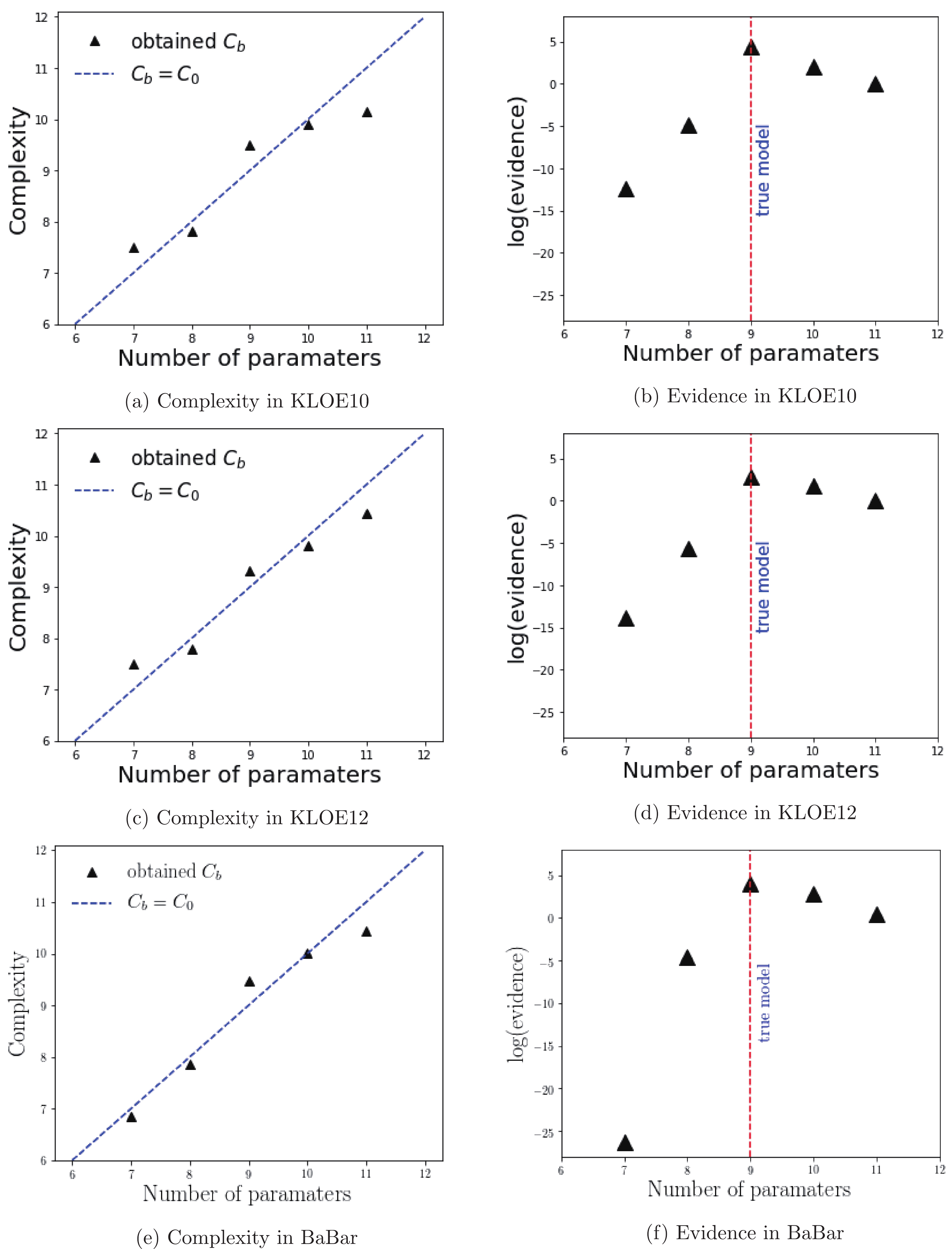
Figure 4. (color online) Summaries of the KLOE10, KLOE12, and BaBar analyses using fit
$ A\text{-}N\rho $ . The plots in the left-hand column depict the complexity against the number of parameters meanwhile the ones in the right-hand column are the logarithm of the evidence as a function of the number of parameters. The red lines indicate that$ C_{0} = 9 $ (linear polynomial) is favored by the three data.
Figure 5. (color online) Summaries of the CMD2, SND, and BESIII analyses using fit
$A\text{-}N\rho$ . The plots for CMD2 consistently favor the linear model. Following Occam's razor, the plateau region within both the log-evidence and the complexity plots for SND implies that the linear model should be selected. BESIII plots provide an inconclusive answer owing to the apparent inconsistency between the complexity plot and the log-evidence plot. -
Referring to Figs. 4(a) and 4(b) for KLOE10, we could still incorporate at least the second order polynomial in our analysis although we observed that the fit
$A\text{-}N\rho$ may oppose this. However, the data were consistently unable to support the cubic polynomial, as all the obtained complexities were smaller than$ {\cal{C}}_{0}(C) = 11 $ . When evidence$ p({\bf{y}}\lvert {\cal{M}}) $ was used in our analysis, we observed that the data demonstrated high preference for the linear-polynomial scenario,$ {\cal{C}}_{0}(L) \gg {\cal{C}}_{0}(Q) $ and$ {\cal{C}}_{0}(L) \gg {\cal{C}}_{0}(C) $ . The results held in all fits except the fit A-W$ \rho $ where the Bayesian evidence had only a slight preference for the linear model owing to$ p({\bf{y}}\lvert {\cal{M}}_{L})\approx p({\bf{y}}\lvert {\cal{M}}_{Q}) \approx p({\bf{y}}\lvert {\cal{M}}_{C}) $ . We also made the same inference for the KLOE12 data as we observed that the effective complexity could only penalize the cubic polynomial (Figs. 4(c) and 4(d)). Moreover, the evidence-based computation also indicated that the linear scenario was also favored, regardless of the priors. The conclusion based on these values in KLOE12 analysis may be weaker compared with the KLOE10 data since the$ {\cal{C}}_{0}(L) $ in the KLOE12 scenario was only a few times larger than$ {\cal{C}}_{0}(Q) $ . -
A significant decrease in the model probability was also observed for the BaBar results (Table 2 and Figs. 4(e) and 4(f)) while the effective complexity increased at a low rate — a similar behavior that we observed in the previous KLOE10 and KLOE12 analyses. Thus, we similarly neglected the more complex models and retained the linear polynomial in our pion form factor analysis. In addition, all fits for the KLOE10, KLOE12, and BaBar data undoubtedly supported the selection of linear polynomial, which was apparent from the fitted values of both
$ \beta $ and$ \gamma $ tabulated in the Table 2, i.e., the values were consistent with zero within 1$ \sigma $ . -
The Bayesian analysis on the CMD2 data revealed that the linear scenario might be the desired one: the complexity increased gradually but the probability did not (Figs. 5(a) and 5(b)). In contrast, the evidence of the SND analysis retained the same magnitude in all considered polynomials (Figs. 5(c) and 5(d)). Incorporating the effective complexity, we selected the simplest model with the smallest number of free parameters, i.e, the linear polynomial because the quality of fit was inadequate to offset the Occam's razor penalty factor.
-
An apparent discrepancy was observed between the complexity and number of parameters in the BESIII analysis as the argument
$ {\cal{C}}_{b}<{\cal{C}}_{0} $ held in all fits (Table 3 and Figs. 5(e) and 5(f)). The complexity increased significantly slower than that of the previous data, indicated by the constant values of the evidence$ p({\bf{y}}\lvert {\cal{M}}) $ . The inclusion of the higher order terms seldom improved the model evidence by any means. The fit B-N$ \rho $ may be exempted from this problem, but the fit A-N$ \rho $ implied that the difference of the evidence to the fit B-N$ \rho $ suggested that the calculation may depend on the prior we consider. Remember that the results obtained from different priors (with also slightly different inputs) ought to agree to provide the same inference. This was not observed between fits A-N$ \rho $ and B-N$ \rho $ ; thus, we cannot provide a conclusive answer solely from the evidence. Additionally, we performed a diagnosis to examine whether the BESIII data was unable to constraint nine or more free parameters in our approach by considering a reformulation of the charge radius in terms of$ \alpha $ , namely$ \kappa_{1} = m_{\omega}^{2}\left( \frac{1}{6}\langle r_{V}^{2} \rangle - \alpha - \frac{1}{\pi}\int_{4m_{\pi}^{2}}^{\infty} \frac{\delta_{1}(z, \theta_{M})}{z^{2}}\,{\rm{d}}z \right). $

(22) Thus, we had an eight-parameter scenario,
$ {\cal{M}}_{8} $ , in which the value of$ \alpha $ was set to zero. The analysis of$ {\cal{M}}_{8} $ might be used to observe the possible value of the effective complexity of the BESIII data. We denote the Bayes factor$ B_{89} $ as a ratio between the eight-parameter scenario (without any polynomial$ P(s) $ ) and the nine-parameter scenario (the linear polynomial) with$ \kappa_{1} $ eliminated instead of$ \alpha $ (Table 4). The conclusion still holds: a seven-parameter model might be favored by the BESIII data.Fit $ B_{89} $ 

$ {\cal{C}}_{b} $ 

A-W $ \rho $ 

23.63 7.05 A-N $ \rho $ 

36.10 7.05 Table 4. Complexity and evidence of the BESIII data using the prior
$ \pi_{A} $ with$ \langle r_{V}^{2} \rangle $ formulated via Eq. (22). The evidences are evaluated for the eight-parameter scenario,$ {\cal{M}}_{8} $ .$ B_{89} $ denotes the Bayes factor between$ {\cal{M}}_{8} $ and$ {\cal{M}}_{9} $ (the linear case).We further augmented the analysis of the complexity by performing "additional fits" to construct two additional models: an eight-parameter model and a seven-parameter model. First, we set the value of the total width (
$ \Gamma_{\omega} $ ) to$ (8.49\pm 0.08) $ MeV (the average values from the PDG [31]) to obtain the eight-parameter model. Subsequently, a seven-parameter model was formulated by fixing the value of$ \omega $ mass using the PDG value. We continued the SDDR procedure, beginning from the results of the linear scenario (the nine-parameter model), to infer the eight-parameter and seven-parameter scenarios. We only demonstrate the analysis in which the prior for$ \kappa_{1} $ was selected to be from$ \pi_{A} $ . We note that the complexity based analysis for BESIII, depicted in Fig. 5(e), also favored the seven-parameter scenario. This confirms our previous analysis in Table 3. -
We only quote the radii of the linear scenario, which was favored by the previous model selection procedure. First, we considered averaging the radii obtained from each prior selection in one dataset, and each value from the data was considered to be a "separate experiment" (i.e., we generated two radius values for each dataset: one from W
$ \rho $ and the other from N$ \rho $ ). Therefore, we achieved 12 measured points,$ n_{\rm{points}} = 12 $ , for each phase shift input: N$ \rho $ and W$ \rho $ . The radii were then combined using the weighted average formula from which we could also extract the error via the "weights,"$ w_{i} $ [31]. If we assume independent (uncorrelated) measurements, the expression becomes$ \langle r_{V}^{2} \rangle_{\rm{ave}} = \frac{\displaystyle\sum_{i} w_{i}\langle r_{V}^{2} \rangle_{i}}{\displaystyle\sum_{i}w_{i}} \quad{,}\quad w_{i} = (1/\epsilon_{i})^{2}, $

(23) where
$ \epsilon_{i} $ denotes the individual uncertainty of the$i {\rm{th}}$ measurement. The combined error,$ \delta\langle r_{V}^{2} \rangle $ , is expressed as$ \delta\langle r_{V}^{2} \rangle = \left(\sum\limits_{i}w_{i}\right)^{-1/2}. $

(24) We can also compute
$ S = \displaystyle\sum_{i}w_{i}(\langle r_{V}^{2} \rangle_{\rm{ave}}-\langle r_{V}^{2} \rangle_{i})^{2} $ and compare it with the quantity$ \overline{S} = n_{\rm{points}}-1 $ , i.e., S value if the measurements are obtained from a perfect Gaussian distribution. The ratio$ S/\overline{S} $ indicates the extent to which we may select the average value to represent the combined measurements. In all our scenarios, we had$ (S/\overline{S})>1 $ , implying that we could still use the average value, but we had to increase the error stated in Eq. (24) by a$ scaling \;factor $ defined as$ \sqrt{S/(n_{\rm{points}}-1)} $ [31]. Because of the insufficient support for the BESIII result deduced via our model selection approach, we omitted the result from the BESIII analysis in averaging the radii. We obtained the radii from fits$W\rho$ and$N\rho$ as$\langle r_{V}^{2} \rangle_{W\rho} = $ $ (0.4472\pm 0.0015)\;{\rm{ fm}}^{2}$ and$\langle r_{V}^{2} \rangle_{N\rho} = (0.4394\pm $ $ 0.0016)\;{\rm{ fm}}^{2}$ , respectively.We further unified the extracted value of
$ \langle r_{V}^{2} \rangle $ by averaging the two values from W$ \rho $ and N$ \rho $ , respectively, in the linear scenario. Excluding the results of the BESIII analysis, we obtained$ \langle r_{V}^{2} \rangle = (0.4436 \pm 0.0039)\;{\rm{ fm}}^{2} $ , where a scaling factor of 3.6 was applied for the uncertainty. We could compare this with the individual values in Fig. 6. Finally, the pion charge radius$ \sqrt{\langle r_{V}^{2} \rangle} $ became
Figure 6. (color online) Total average values of the squared pion charge radius in which the BESIII radius is excluded. This value are compared with the ones from the other datasets (including the BESIII value). The thick horizontal lines indicate the total mean value.
$ \sqrt{\langle r_{V}^{2} \rangle} = (0.6660 \pm 0.0029)\;{\rm{ fm}}. $

(25) The value was consistent within 1
$ \sigma $ with the recent PDG average value ($ 0.659 \pm 0.004 $ ) fm. -
As of 2020, the most updated radius values in the PDG were contributed from the systematic and comprehensive result by Colangelo et al. that included both time-like and space-like datasets for the analysis [4]. Their value reads
$ \langle r_{V}^{2}\rangle_{\rm{Colangelo}} = (0.429 \pm 0.004) {\rm{ fm}}^{2}. $

(26) Colangelo's value is also consistent with the early value obtained by Ananthanarayan et al., which utilized a rigorous optimization technique and Monte Carlo simulations [2]. However, our obtained value is too close to the edge of
$ 2\sigma $ of their value, implying an inconsistency indicated by Colangelo et al. owing to some apparent challenges in formulating our problem. One of them is the simplified and outdated version of the Omnès formulation of the pion vector form factor.Based on the discussion by Colangelo et al., the polynomial described in our approach must describe how the inelasticities are open above
$ s_{\rm{in}} = (m_{\pi}+m_{\omega})^{2} $ . This is described by a branch-cut singularity at$ s = s_{\rm{in}} $ . Therefore, the polynomial part in Eq. (7) must be generalized as a conformal polynomial instead of a simple polynomial expansion. It is expressed as$ P_{\rm in}(s) = 1 + \sum\limits_{k = 1}^{N} c_{k}(z^{k}(s) - z^{k}(0)) , $

(27) where
$ c_{k} $ denotes fit parameters where N must be specified. Moreover, s is conformally transformed into$ z(s) $ as$ z(s) = \frac{\sqrt{s_{\rm{in}} - s_{c}} -\sqrt{s_{\rm{in}} - s}}{\sqrt{s_{\rm{in}} - s_{c}} + \sqrt{s_{\rm{in}} - s}}, $

(28) where
$ s_{c} $ is an auxiliary variable selected to be varied from −0.5 GeV2 to −2.0 GeV2. Furthermore, the$ \rho-\omega $ mixing effect must be revised to include a correct right-hand cut behavior at$ s = 9m_{\pi}^{2} $ [4], i.e.,$ G_{\omega}(s) = 1 + \frac{s}{\pi}\int_{9m_{\pi}^{2}}^{\infty} \frac{{\rm{Im}}g_{\omega}(s')}{s'(s'-s)}\left(\frac{1-\dfrac{9m_{\pi}^{2}}{s'}}{1-\dfrac{9m_{\pi}^{2}}{m_{\omega}^{2}}}\right)^{4}, $

(29) where
$ g_{\omega} $ resembles a somewhat similar Breit-Wigner parameterization that we discussed in Eq. (7), which reads as$ g_{\omega}(s) = 1 + \kappa_{1}\frac{s}{\left(m_{\omega}-\dfrac{\rm i}{2}\Gamma_{\omega}\right)^{2}-s}. $

(30) Hence, we performed an additional computation that employed a more sophisticated formulation of the pion vector form factor described by Colangelo et al.
$ F_{V}(s) = P_{\rm in}(s)G_{\omega}(s)\Omega(s). $

(31) For a quick comparison, we only input the phase shift
$ {W}\rho $ into Eq. (31).As dictated by Colangelo et al., using a polynomial order
$ N>3 $ does not provide a good estimate for the radius computation because the oscillation of the complex phase of the conformal polynomial becomes larger as N increases. This should be possible to investigate using the previous Bayesian model selection technique we used. However, since we are only interested in providing a simple and somewhat intuitive comparison with the existing results, we only discuss the result for$ P_{\rm{in}}(s) $ with$ N = 2 $ and$ N = 3 $ . We consider the polynomial only up to$ N = 3 $ (cubic term). To retrieve the correct P-wave behavior near$ s = s_{\rm{in}} $ , we should have$ c_{1} = -\sum_{k = 2}^{N} k c_{k} $ . Thus, we only require to asses two models, namely$ N-1 = 1 $ (quadratic) and$ N-1 = 2 $ (cubic). In addition, we can equivalently parameterize one of the polynomial coefficients, for example$ c_{2} $ , with$ \langle r_{V}^{2}\rangle $ using the sum rule from Eq. (8), i.e.,$ c_{2} = f(\langle r_{V}^{2}\rangle) $ where f is some function. Hence, we can ignore$ c_{2} $ completely from our discussion and set$ c_{3} = 0 $ instead when we refer to the quadratic model.Moreover, we place only an uninformative prior onto
$ c_{3} $ in a similar fashion to the parameters$ \beta $ or$ \gamma $ . The upper and lower limits of$ c_{3} $ to define a flat prior are obtained from the results in Colangelo et al. The prior should be combined with a constraint for$ c_{k} $ obtained via the Eidelman–Łukaszuk (EŁ) bound [32]. However, in this paper, we aim to make a simple and rapid observation to compare radii obtained from the new$ F_{V} $ formulation; hence, we assume the fit values in [4] are sufficient for our objective. We utilize a simple flat prior for$ s_{c} $ :$ \pi(s_{c})\sim 1 $ for$ -2.0\leqslant s_{c} \leqslant -0.5 $ and append a decay behavior beyond this range.We performed the Bayesian parameter inference using this new
$ F_{V} $ formulation. The results are summarized in Table 5. We observed that our fitted$ c_{3} $ values corroborated with the results of Colangelo et al. within$ 1\sigma $ . Moreover, the radius values generally increased for the cubic model than the quadratic model except for the KLOE12 result. We also observed relatively larger values for KLOE10, KLOE12, and BESIII compared with values from the previous formulation (see Fig. 6 and the supplemental tables). Despite the apparent difference in the phase shift input between Colangelo's result and ours, we must further explore in a future analysis whether the new formulation (i.e., the conformal polynomial and the isospin factor) or the phase shift contributes mostly to the results. To check the latter, we could directly use the Regge based formulation described in [33] for the input. Another approach would be to incorporate a new extended Madrid phase shift in [34] that may provide a testament for better radius extractions in the framework of the Bayesian inference. The results from the current and the previous analysis demonstrate that the Gaussian assumption of the marginal distribution of Madrid parameters$ \theta_{M} $ might not be always correct. This is particularly true for more complex model(s), i.e., quadratic and/or cubic models. This should be addressed by permitting non-Gaussian priors for the Madrid parameters. The nature of non-Gaussian errors of these parameters are also discussed in [35] and will be investigated further in our future analysis.Data $N-1$ 

$\langle r_{V}^{2}\rangle$ /fm2

$\kappa\times 10^{-3}$ 

$c_{3}$ 

KLOE10 1 0.4764(26) 1.20(4) − 2 0.4878(29)(26) 1.21(4) 0.1(1) KLOE12 1 0.4869(29)(26) 1.21(10)(9) − 2 0.4526(77)(64) 1.03(8) −0.2(1) BaBar 1 0.4420(12)(13) 1.33(3) − 2 0.4482(53)(45) 1.33(3) −0.06(6) CMD2 1 0.4365(21)(23) 1.18(5) − 2 0.4539(11)(9) 1.17(5) −0.2(1) SND 1 0.4400(17) 1.30(4) − 2 0.4697(13)(11) 1.28(4) −0.3(1) BESIII 1 0.4810(29)(26) 1.23(11) − 2 0.4716(32)(27) 1.22(10) −0.5(4) Table 5. Parameter estimation using the pion vector form factor formulated in Eq. (31) using fits for the quadratic (
$N-1=1$ ) and cubic model ($N-1=2$ ).Several problems with our values may relate to our oversimplified data considerations. We omitted the off-diagonal covariance matrices for BaBar and KLOEs from our analysis to simplify our likelihood formulation (i.e., Eq. (13)). Next, we ignored the outlier analysis of the datasets which may be important in this scenario because Colangelo et al. performed the fits by considering potential outliers on the data as one of the of systematic errors. In addition, the data with undressed vacuum polarization effects included in the sets must be addressed in a future analysis using this Bayesian approach.
-
In this study, we employed a Bayesian inference to extract the value of the pion charge radius based on the dispersion relations, utilizing several experimental
$ e^{+}e^{-} $ datasets. We used two phase shifts for the pion vector form, and they differ slightly in terms of continuation function above 1.3 GeV2. Our Bayesian inference is constructed upon two types of priors, namely informative and non-informative priors, which are useful to avoid bias from any particular choices of the prior distribution. We computed the posterior distribution numerically for each prior information by using the MCMC algorithm to infer model parameters in the pion form factor, including the pion charge radius.In addition, the nested model problem was addressed using Bayesian model selection to compare the model evidences of the polynomial choices. An economically straightforward approach to compute the evidence of the nested models involved the use of SDDR with the existing MCMC samples of the posterior distribution. This can also be achieved through nested sampling [36] for general non-nested models. In practice, we computed the model evidence via the MULTINEST algorithm, which is a popular multimodal nested sampling method developed by Feroz et al. [37]; the conclusion drawn from the SDDR method agrees with the computations from MULTINEST that favors the linear polynomial. Moreover, effective complexity was used to infer the number of parameters permitted by the data combined with the model evidences. However, a more robust approach that involves Bayesian dimensionality introduced by Handley et al. [18] may provide an alternative to compute the improved version of the effective complexity. Our analyses reveal that the nine-parameter model (linear polynomial) of the pion vector form factor is more favored to extract the pion charge radius.
In addition to the comparison of our result with of the most updated values from Colangelo et al., we must address the computational burden of our Bayesian approach despite having a more intuitive applicability in addressing parameter estimation (radius extraction) and model selection (determine polynomial order). Our posterior sampling may be expensive to compute, and thus hinder the wider applications of this framework to improve the fitting procedure used in the dispersion relations. However, we argue that an approximate Bayesian computation (APC) could serve as a faster and lighter alternative method to our conventional approach [38-40]. In addition, high-peformance parallel optimization techniques for Bayesian methods that may permit for faster hyperparameter tunings in a grander scale in the realms of particle physics research should be developed (for an interesting example, refer to Ref. [41]).
-
The authors wish to thank Andreas Wirzba, Christoph Hanhart, and Bastian Kubis for providing helpful discussions on the underlying physics concepts and the Bayesian formulations.
-
The following tables summarize the results from all fits for different numbers of parameters denoted by
${\cal{C}}_{'}$ (i.e., 9, 10, and 11) using the original formulation of$F_{V}$ . We only indicate the parameter inference for the pion radius charge ($\langle r_{V}^{2}\rangle$ ) and three "polynomial parameters" (i.e.,$\kappa$ ,$\beta$ , and$\gamma$ ), including their uncertainty. The model evidences and effective complexities presented in the tables were obtained from the SDDR based procedure to solve the nested model problem in our analysis. The values of the Akaike Information Criterion (AIC) and Bayesian Information Criterion (BIC) are shown here to achieve completeness.Prior Resonance ${\cal{M}}$ (

${\cal{C}}_{0}$ )

$\langle r_{V}^{2}\rangle$ /fm2

$\kappa\times 10^{-3}$ 

$\beta$ /GeV

$^{-4}$ 

$\gamma$ /GeV

$^{-6}$ 

AIC BIC $p({\bf{y}}\lvert {\cal{M}})$ 

${\cal{C}}_{b}$ 

$\pi_{A}$ 

Fit $A\text{-}W\rho$ 

L (9) 0.4412(22) 1.71(7) $0^{*}$ 

$0^{*}$ 

88.2 109.0 9.35 9.36 Q (10) 0.4352(44) 1.76(8) 0.08(5) $0^{*}$ 

91.7 114.9 3.83 9.56 C (11) 0.4332(116) 1.76(8) 0.1(2) 0.0(1) 97.7 123.2 1.00 9.90 Fit $A\text{-}N\rho$ 

L (9) 0.4328(22) 1.71(7)(7) $0^{*}$ 

$0^{*}$ 

87.9 108.8 55.90 8.96 Q (10) 0.4307(42) 1.73(8) 0.03(5) $0^{*}$ 

91.7 114.9 3.39 9.38 C (11) 0.4245(114)(117) 1.73(8) 0.1(2) 0.0(1) 94.3 119.8 1.00 10.00 $\pi_{B}$ 

Fit $B\text{-}W\rho$ 

L (9) 0.4409(22) 1.68(7) $0^{*}$ 

$0^{*}$ 

87.9 108.8 80.00 9.50 Q (10) 0.4368(39)(42) 1.73(8) 0.05(5)(4) $0^{*}$ 

103.7 126.9 7.63 9.90 C (11) 0.4311(132) 1.74(8) 0.01(2) 0.0(2)(1) 93.7 119.2 1.00 10.15 Fit $B\text{-}N\rho$ 

L (9) 0.4325(23) 1.69(7) $0^{*}$ 

$0^{*}$ 

88.0 108.8 202.10 9.51 Q (10) 0.4335(34) 1.73(8)(7) 0.00(3)(4) $0^{*}$ 

89.5 112.7 7.86 9.69 C (11) 0.4249(118)(101) 1.71(8) 0.1(1)(2) 0.0(1) 120.3 145.8 1.00 10.10 Table 6. Bayesian analysis of the KLOE10 data employing two different priors: informative and uninformative (denoted by
$\pi_{A}$ and$\pi_{B}$ ) and two different phase shift inputs with higher$\rho$ resonances ($W\rho$ ) and without higher$\rho$ resonances ($N\rho$ ). To avoid cluttering the notation, we establish the "fits" A-W$\rho$ , A-N$\rho$ , B-W$\rho$ , and B-N$\rho$ to denote the combination of the prior and the phase shift.Prior Resonance ${\cal{M}}$ (

${\cal{C}}_{0}$ )

$\langle r_{V}^{2}\rangle$ /fm2

$\kappa\times 10^{-3}$ 

$\beta$ GeV

$^{-4}$ 

$\gamma$ /GeV

$^{-6}$ 

AIC BIC $p({\bf{y}}\lvert {\cal{M}})$ 

${\cal{C}}_{b}$ 

$\pi_{A}$ 

Fit $A\text{-}W\rho$ 

L (9) 0.4451(21) 1.61(11) $0^{*}$ 

$0^{*}$ 

85.2 104.0 13.03 9.28 Q (10) 0.4382(50)(52) 1.64(12) 0.08(6)(5) $0^{*}$ 

87.2 108.2 3.36 9.67 C (11) 0.4310(130) 1.63(12) 0.2(2) 0.0(1) 90.4 113.4 1.00 10.08 Fit $A\text{-}N\rho$ 

L (9) 0.4372(22) 1.62(11) $0^{*}$ 

$0^{*}$ 

84.0 102.8 16.65 9.20 Q (10) 0.4352(46)(50) 1.63(12) 0.03(6)(5) $0^{*}$ 

85.6 106.5 2.38 9.61 C (11) 0.4220(128)(130) 1.61(12) 0.2(2) −0.1(1) 89.9 112.9 1.00 9.94 $\pi_{B}$ 

Fit $B\text{-}W\rho$ 

L (9) 0.4448(21) 1.54(12) $0^{*}$ 

$0^{*}$ 

84.4 103.3 18.24 9.32 Q (10) 0.4407(42)(48) 1.56(12) 0.05(5)(4) $0^{*}$ 

105.0 125.9 6.00 9.81 C (11) 0.4263(144) 1.55(13) 0.2(2) −0.1(1) 100.3 123.3 1.00 10.44 Fit $B\text{-}N\rho$ 

L (9) 0.4370(22) 1.54(12) $0^{*}$ 

$0^{*}$ 

84.0 103.0 59.4 9.29 Q (10) 0.4355(46)(49) 1.56(16) 0.02(6)(5) $0^{*}$ 

86.9 107.8 3.71 9.18 C (11) 0.4170(142)(141) 1.52(12) 0.3(2) −0.2(1) 97.2 120.3 1.00 10.15 Table 7. Bayesian analysis of the KLOE12 data employing two different priors: informative and uninformative (denoted by
$\pi_{A}$ and$\pi_{B}$ ) and two different phase shift inputs with higher$\rho$ resonances ($W\rho$ ) and without higher$\rho$ resonances ($N\rho$ ). To avoid cluttering the notation, we establish the "fits" A-W$\rho$ , A-N$\rho$ , B-W$\rho$ , and B-N$\rho$ to denote the combination of the prior and the phase shift.Prior Resonance ${\cal{M}}$ (

${\cal{C}}_{0}$ )

$\langle r_{V}^{2}\rangle$ /fm2

$\kappa\times 10^{-3}$ 

$\beta$ /GeV

$^{-4}$ 

$\gamma$ /GeV

$^{-6}$ 

AIC BIC $p({\bf{y}}\lvert {\cal{M}})$ 

${\cal{C}}_{b}$ 

$\pi_{A}$ 

Fit $A\text{-}W\rho$ 

L (9) 0.4430(35)(33) 1.81(14) $0^{*}$ 

$0^{*}$ 

58.2 77.1 0.89 7.28 Q (10) 0.4232(93)(96) 1.81(15)(14) 0.18(8) $0^{*}$ 

57.5 78.4 1.82 8.09 C (11) 0.4050(216)(213) 1.87(15) 0.5(3) −0.2(3) 58.1 81.2 1.00 8.54 Fit $A\text{-}N\rho$ 

L (9) 0.4328(31) 1.79(14) $0^{*}$ 

$0^{*}$ 

57.2 76.0 1.94 7.13 Q (10) 0.4185(91) 1.83(14) 0.13(8) $0^{*}$ 

57.3 80.5 1.11 7.98 C (11) 0.3976(219)(215) 1.84(14) 0.5(3) −0.3(3) 57.8 83.3 1.00 8.40 $\pi_{B}$ 

Fit $B\text{-}W\rho$ 

L (9) 0.4423(35)(33) 1.73(15) $0^{*}$ 

$0^{*}$ 

58.4 77.2 3.27 7.37 Q (10) 0.4230(95)(97) 1.79(16) 0.05(5)(4) $0^{*}$ 

57.4 78.3 1.13 7.92 C (11) 0.3577(371)(373) 1.80(16) 0.2(2) −0.1(1) 55.4 78.5 1.00 7.78 Fit $B\text{-}N\rho$ 

L (9) 0.4321(34) 1.71(15) $0^{*}$ 

$0^{*}$ 

57.0 75.8 9.62 7.39 Q (10) 0.4148(94)(92) 1.76(15) 0.1(1) $0^{*}$ 

57.2 80.7 0.91 8.24 C (11) 0.3493(365)(371) 1.77(16) 1.2(6)(5) −0.9(5)(4) 56.5 82.0 1.00 8.13 Table 8. Bayesian analysis of the BESIII data employing two different priors: informative and uninformative (denoted by
$\pi_{A}$ and$\pi_{B}$ ) and two different phase shift inputs with higher$\rho$ resonances ($W\rho$ ) and without higher$\rho$ resonances ($N\rho$ ). To avoid cluttering the notation, we establish the "fits" A-W$\rho$ , A-N$\rho$ , B-W$\rho$ , and B-N$\rho$ to denote the combination of the prior and the phase shift.Prior Resonance ${\cal{M}}$ (

${\cal{C}}_{0}$ )

$\langle r_{V}^{2}\rangle$ /fm2

$\kappa\times 10^{-3}$ 

$\beta$ /GeV

$^{-4}$ 

$\gamma$ /GeV

$^{-6}$ 

AIC BIC $p({\bf{y}}\lvert {\cal{M}})$ 

${\cal{C}}_{b}$ 

$\pi_{A}$ 

Fit A-W $\rho$ 

L (9) 0.4491(11) 1.86(5) $0^{*}$ 

$0^{*}$ 

219.5 251.8 9.02 9.63 Q (10) 0.4446(26) 1.95(6)(6) 0.08(4) $0^{*}$ 

220.2 256.2 5.47 10.16 C (11) 0.4452(51) 1.95(7)(7) 0.07(7) 0.00(8) 223.4 263.0 1.00 10.32 Fit A-N $\rho$ 

L (9) 0.4417(11) 1.89(5) $0^{*}$ 

$0^{*}$ 

219.4 251.8 21.44 9.33 Q (10) 0.4390(25) 1.94(6) 0.09(7) $0^{*}$ 

220.4 256.4 4.28 9.86 C (11) 0.4359(48) 1.92(7) 0.05(4) −0.05(6) 223.6 266.8 1.00 10.13 $\pi_{B}$ 

Fit B-W $\rho$ 

L (9) 0.4492(11) 1.86(5) $0^{*}$ 

$0^{*}$ 

219.5 251.8 54.46 9.48 Q (10) 0.4448(26) 1.95(6) 0.08(4) $0^{*}$ 

218.8 254.7 16.02 10.01 C (11) 0.4455(47) 1.95(7) 0.07(7) 0.00(8) 227.1 266.6 1.00 10.45 Fit B-N $\rho$ 

L (9) 0.4418(11) 1.89(5) $0^{*}$ 

$0^{*}$ 

219.4 251.8 151.20 9.13 Q (10) 0.4391(24)(25) 1.93(6) 0.05(4) $0^{*}$ 

219.5 255.5 12.45 9.54 C (11) 0.4366(46)(45) 1.95(7) 0.07(7) 0.01(7) 221.9 261.5 1.00 10.83 Table 9. Bayesian analysis of the BaBar data employing two different priors: informative and uninformative (denoted by
$\pi_{A}$ and$\pi_{B}$ ) and two different phase shift inputs with higher$\rho$ resonances ($W\rho$ ) and without higher$\rho$ resonances ($N\rho$ ). To avoid cluttering the notation, we establish the "fits" A-W$\rho$ , A-N$\rho$ , B-W$\rho$ , and B-N$\rho$ to denote the combination of the prior and the phase shift.Prior Resonance ${\cal{M}}$ (

${\cal{C}}_{0}$ )

$\langle r_{V}^{2}\rangle$ /fm2

$\kappa\times 10^{-3}$ 

$\beta$ /GeV

$^{-4}$ 

$\gamma$ /GeV

$^{-6}$ 

AIC BIC $p({\bf{y}}\lvert {\cal{M}})$ 

${\cal{C}}_{b}$ 

$\pi_{A}$ 

Fit A-W $\rho$ 

L (9) 0.4505(37) 1.71(7) $0^{*}$ 

$0^{*}$ 

50.3 62.6 4.47 9.25 Q (10) 0.4425(75)(78) 1.75(8) 0.07(7) $0^{*}$ 

53.2 66.9 1.12 9.45 C (11) 0.4157(225)(219) 1.74(8) 0.4(3) −0.2(2) 53.3 68.3 1.00 10.16 Fit A-N $\rho$ 

L (9) 0.4412(37) 1.71(7) $0^{*}$ 

$0^{*}$ 

50.6 62.9 6.16 9.46 Q (10) 0.4400(71)(73) 1.72(8) 0.01(7) $0^{*}$ 

52.6 66.3 0.77 9.50 C (11) 0.4078(212)(217) 1.71(8) 0.4(3) −0.3(2) 52.5 67.5 1.00 10.18 $\pi_{B}$ 

Fit B-W $\rho$ 

L (9) 0.4500(37)(36) 1.71(7) $0^{*}$ 

$0^{*}$ 

50.3 62.6 23.39 9.20 Q (10) 0.4426(74)(77) 1.75(8) 0.08(7)(6) $0^{*}$ 

57.3 71.0 1.49 9.58 C (11) 0.4200(206)(208) 1.74(8) 0.3(3) −0.2(2) 55.3 70.4 1.00 9.53 Fit B-N $\rho$ 

L (9) 0.4407(37) 1.71(7) $0^{*}$ 

$0^{*}$ 

50.6 62.9 11.00 9.24 Q (10) 0.4404(72)(75) 1.72(8) 0.01(7) $0^{*}$ 

52.6 66.3 0.42 9.49 C (11) 0.3828(281)(289) 1.70(8) 0.8(4) −0.5(2) 53.8 68.8 1.00 9.58 Table 10. Bayesian analysis of the CMD2 data employing two different priors: informative and uninformative (denoted by
$\pi_{A}$ and$\pi_{B}$ ) and two different phase shift inputs with higher$\rho$ resonances ($W\rho$ ) and without higher$\rho$ resonances ($N\rho$ ). To avoid cluttering the notation, we establish the "fits" A-W$\rho$ , A-N$\rho$ , B-W$\rho$ , and B-N$\rho$ to denote the combination of the prior and the phase shift.Prior Resonance ${\cal{M}}$ (

${\cal{C}}_{0}$ )

$\langle r_{V}^{2}\rangle$ /fm2

$\kappa\times 10^{-3}$ 

$\beta$ /GeV

$^{-4}$ 

$\gamma$ /GeV

$^{-6}$ 

AIC BIC $p({\bf{y}}\lvert {\cal{M}})$ 

${\cal{C}}_{b}$ 

$\pi_{A}$ 

Fit A-W $\rho$ 

L (9) 0.4469(27) 1.78(6) $0^{*}$ 

$0^{*}$ 

84.4 100.7 0.16 9.26 Q (10) 0.4339(60)(64) 1.88(7) 0.15(7)(6) $0^{*}$ 

84.6 102.7 0.37 9.19 C (11) 0.4030(160)(158) 1.86(7) 0.6(2) −0.3(2) 80.2 100.0 1.00 9.30 Fit A-N $\rho$ 

L (9) 0.4382(28)(27) 1.79(6) $0^{*}$ 

$0^{*}$ 

85.5 101.7 0.54 8.48 Q (10) 0.4310(57)(60) 1.84(7) 0.08(6) $0^{*}$ 

86.9 105.0 0.16 9.46 C (11) 0.3949(156) 1.83(7) 0.6(2) −0.4(2) 81.9 101.8 1.00 9.85 $\pi_{B}$ 

Fit B-W $\rho$ 

L (9) 0.4469(27) 1.76(6) $0^{*}$ 

$0^{*}$ 

84.7 101.0 0.45 9.00 Q (10) 0.4339(59)(63) 1.88(7) 0.15(7) $0^{*}$ 

81.7 99.8 0.46 9.36 C (11) 0.4070(154) 1.86(7) 0.7(2) 0.4(2) 84.7 104.6 1.00 9.61 Fit B-N $\rho$ 

L (9) 0.4379(28) 1.79(6) $0^{*}$ 

$0^{*}$ 

85.5 101.7 4.55 9.44 Q (10) 0.4310(57)(60) 1.84(7) 0.08(6) $0^{*}$ 

84.1 102.2 0.23 9.83 C (11) 0.3984(151)(147) 1.82(7) 0.5(2) −0.3(2)(1) 80.8 100.6 1.00 10.26 Table 11. Bayesian analysis of the SND data employing two different priors: informative and uninformative (denoted by
$\pi_{A}$ and$\pi_{B}$ ) and two different phase shift inputs with higher$\rho$ resonances ($W\rho$ ) and without higher$\rho$ resonances ($N\rho$ ). To avoid cluttering the notation, we establish the "fits" A-W$\rho$ , A-N$\rho$ , B-W$\rho$ , and B-N$\rho$ to denote the combination of the prior and the phase shift.
A Bayesian-based approach for extracting the pion charge radius from electron-electron scattering data
- Received Date: 2021-01-05
- Available Online: 2021-08-15
Abstract: In this study, we utilize a potentially versatile Bayesian parameter approach to compute the value of the pion charge radius and quantify its uncertainty from several experimental


 DownLoad: