


 Abstract
 HTML
HTML Reference
 Related
 PDF
PDF


-
The LHCb collaboration recently reported an observation of the doubly charmed baryon
$ \Xi_{cc}^{++}(ccu) $ in the$ \Lambda^+_cK^-\pi^+\pi^+ $ decay channel, where the mass and lifetime of the baryon are determined as$ 3.621 $ GeV [1] and 0.256 ps [2]. A systematic theoretical research of the kindred baryons (doubly heavy baryons) thus became imperative. In addition, LHCb also reported observations of five narrow$ \Omega_c^0 $ excited baryons in 2017 [3] and$ \Xi^-_{b} $ in 2018 [4]. In most theoretical models, the mass of the doubly heavy baryon$ \Xi_{cc}^{+(+)} $ is predicted to be in the range$ 3.5\sim3.7 $ GeV [5-18]. The mass splitting between$ \Xi_{cc}^{++} $ and$ \Xi^+_{cc} $ is predicted to be several MeV due to the mass difference of the light quarks$ u $ and$ d $ . The predicted mass in lattice QCD is about 3.6 GeV [19-21], which is quite close to the LHCb observation. The lifetimes of$ \Xi^{+}_{cc} $ and$ \Xi_{cc}^{++} $ are predicted to be quite long,$ 50\sim250 $ and$ 200\sim700 $ fs [22-25], respectively. The LHCb measurement of$ \Xi_{cc}^{++} $ is very close to the lower limit of the theoretical predictions. It is expected that more information about the doubly heavy baryon(s) will be available in the near future.Compared with mesons, baryons as three-quark bound states are much more complicated. However, for a doubly heavy baryon, the two heavy quarks involved move relatively slowly, and are strongly bound with each other forming a color anti-triplet diquark core①. Thus, it is reasonable to reduce the three-body problem to two two-body ones. Due to the Pauli principle, the baryon wave functions must be totally anti-symmetric under the interchange of any two quarks. For the diquark core with an even orbital angle momentum
$ L_{\rm{D}} $ , the spin-flavor part of the wave function must be symmetric. Hence,$ (cc) $ and$ (bb) $ diquarks in the ground state ($ S $ -wave) must have$ J^P = 1^+ $ , while$ (bc) $ diquark, carrying different flavors, may have$ J^P = 1^+ $ or$ 0^+ $ . In this work we focus on$ \frac{1}{2}^+ $ or$ \frac{3}{2}^+ $ baryons with$ 1^+ $ doubly heavy diquark cores ($ cc $ ,$ bc $ or$ bb $ );$ \frac{1}{2}^+ $ baryons with$ 0^+ $ $ (bc) $ diquark, e.g.$ \Xi'_{bc} $ and$ \Omega'_{bc} $ , will be presented elsewhere.Based on the above, we reduce the three-body problem of the doubly heavy baryons to two two-body problems. We first deal with diquark cores in the framework of the Bethe-Salpeter equation (BSE) with the QCD inspired kernel. In the so-called instantaneous approximation, we solve the corresponding three-dimensional (Bethe-)Salpeter equation, and obtain the diquark spectra and wave functions. The second step is to establish a BSE for the diquark core and the remaining light quark, where the structured diquark effects in the BSE kernel are described by the appropriate form factors. The instantaneous approximation is also used to solve the baryon BSE. In this scheme, both steps deal only with two-body (Bethe-)Salpeter equations. In fact, a similar strategy was adopted in Refs. [26-39] but with different methods and approximations. It is known that the BSE framework can be successfully used to study the two-body meson systems, e.g. the mass spectra [40,41], hadronic transitions and electro-weak decays [42-48]. A widespread agreement between the theoretical predictions and experimental observations has been achieved. Our main motivation in this work is to push the BSE approach further, and to develop a precise and systematic method for describing the doubly heavy baryons.
The paper is organized as follows. In Sec. 2, we describe the
$ 1^+ $ diquark BSE in the instantaneous approximation, solve the mass spectra and wave functions, and then compute the diquark form factors in the Mandelstam formulation. In Sec. 3, we derive the three-dimensional diquark-quark (Bethe-)Salpeter equation, and solve the mass spectra and wave functions of baryons with$ J^P = \frac{1}{2}^+ $ and$ \frac{3}{2}^+ $ . In particular, the diquark-core form factors play an important role in determining the BS kernel for the baryons. In Sec. 4, we discuss the results obtained, and compare them with the other sources. Finally, we provide a brief summary of this work. -
Since the QCD inspired interaction kernel for the doubly heavy diquark core has the same origin as for the doubly heavy mesons, we briefly review the latter first. In this work, it is assumed that the instantaneous approximation (IA) works well since the systems considered always involve a heavy quark. In IA, the kernel has no dependence on the time component of the exchanged momentum, and can be expressed as a ‘revised one-gluon exchange’
$ iK_{\rm{M}}(q )\simeq i V_{\rm{M}}(\vec q )\gamma^\alpha \otimes \gamma_\alpha = i\left[V_{\rm{G}}(\vec q )+V_{\rm{S}}(\vec q )\right]\gamma^\alpha \otimes \gamma_\alpha, $

(1) where
$ V_{\rm{G}}(\vec q ) $ is the usual one-gluon exchange potential and$ V_{\rm{S}}(\vec q ) $ is a phenomenological screened potential, which behave in the Coulomb gauge as [49]:$ \begin{split} &V_{\rm{G}}(\vec q ) = -\frac{4}{3} \frac{4\pi \alpha_s(\vec q )}{\vec q ^2+a_1^2},\\ & V_{\rm{S}}(\vec q ) = \left[(2\pi)^3 \delta^3(\vec q )\left( \frac{\lambda}{a_2}+V_0 \right)- \frac{8\pi \lambda}{(\vec q ^2+a_2^2)^2}\right], \end{split}$

(2) where
$ \frac{4}{3} $ is the color factor;$ a_{1(2)} $ is introduced to avoid divergence in the region of small transfer momenta; the screened potential$ V_{\rm{S}}(\vec q ) $ is introduced on phenomenological grounds and is characterized by the string constant$ \lambda $ and the factor$ a_2 $ . This potential originates from the famous Cornell potential [50,51], which expresses the one-gluon exchange Coulomb-type potential at short distance, and a linear growth confinement potential at large distance. In order to incorporate the screening effects [52,53], the confinement potential is modified in the above form [54-56], where$ V_0 $ is a constant fixed by fitting the data. Note that a screened potential containing a time-like vector has been widely used and discussed in many works [57-61], and gives a good description of meson systems. Here, we assume that$ V_{\rm{S}} $ also arises from the gluon exchange and hence carries the same color structure as$ V_{\rm{G}} $ . The strong coupling constant$ \alpha_s $ has the form,$ \alpha_s(\vec q ) = \frac{12\pi}{(33-2N_f)}\frac{1}{\ln\left(a+\dfrac{\vec q ^2}{\Lambda^2_{\rm{QCD}}}\right)}, $

where
$ \Lambda_{\rm{QCD}} $ is the scale of the strong interaction,$ N_f $ is the active flavor number, and$ a = e $ is a constant regulator. For later convenience, we split$ V_{\rm{M}}(\vec q ) $ into two parts,$ V_{\rm{M}}(\vec q ) = (2\pi)^3\delta^3(\vec q )V_{\rm{M1}}+V_{\rm{M2}}(\vec q ), $

(3) where
$ V_{\rm{M1}} $ is a constant and$ V_{\rm{M2}} $ contains all dependence on$ \vec q $ , i.e.,$ V_{\rm{M1}} \equiv \frac{\lambda}{a_2}+V_0 ,\; \; \; V_{\rm{M2}}(\vec q )\equiv - \frac{8\pi \lambda}{(\vec q ^2+a_2^2)^2}-\frac{4}{3} \frac{4\pi \alpha_s(\vec q )}{\vec q ^2+a_1^2}. $

(4) To construct the BSE kernel for a diquark, we need to transform the anti-fermion line into the fermion one by charge conjugation. Considering that the quark-antiquark pair in a meson is a color singlet, while the quark-quark pair inside a baryon is a color anti-triplet, and thus the corresponding color factors are
$ \frac{4}{3} $ and$ -\frac{2}{3} $ , the kernel for the diquark core is simply assumed to be,$ iK_{\rm{D}}(\vec q ) = -\frac{1}{2} iV_{\rm{M}}(\vec q )\gamma^\alpha \otimes (\gamma_\alpha)^{\rm{T}}. $

The ‘half rule’ used here is widely adopted in previous works involving baryons and quark-quark bound systems [8,9,22]. It is exact in the one-gluon exchange limit and has been found to work well in the measurements of the
$ \Xi_{cc}^{++} $ mass. Its successful extension beyond weak coupling implies that the heavy quark potential factorizes into a color-dependent and a space-dependent part, where the latter is the same for quark–quark and quark–antiquark pairs. The relative factor$ \frac{1}{2} $ then results from the color algebra, just as in the weak-coupling limit [62]. Also note that for heavy quarks, compared with the temporal component ($ \alpha = 0 $ ) of the vector-vector$ \gamma^\alpha \otimes \gamma_\alpha $ interaction kernel, the spatial components ($ \alpha = 1,2,3 $ ) are suppressed by a factor$ v\sim \frac{|\vec{p}|}{M} $ , and will be ignored in numerical calculations. This is also consistent with the analysis in Ref. [63]. -
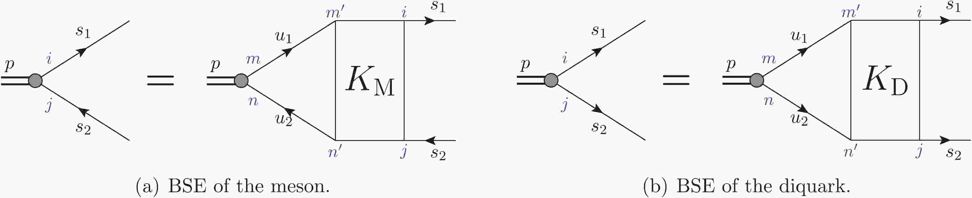
We briefly review the Bethe-Salpeter equation for mesons, as shown in Fig. 1(a), which in the momentum space reads

Figure 1. (color online) BSE of a meson and a diquark.
$p$ denotes the bound state momentum, and$p^2=\mu^2$ , where$\mu$ is the bound system mass;$s_{1(2)}$ and$u_{1(2)}$ are the quark (antiquark) momenta. The blue roman letters denote the Dirac indices.$ \Gamma_{\rm{M}}(p,s) = \int \frac{{\rm{d}}^4 u}{(2\pi)^4} iK_{\rm{M}}(s-u) [S(s_1)\Gamma_{\rm{M}}(p,s)S(-s_2)], $

(5) where
$ \Gamma_{\rm{M}} $ denotes the BS vertex;$ S(s_{1}) $ and$ S(-s_2) $ are the propagators of the quark and antiquark, respectively. The corresponding BS wave function is defined as$ \psi_{\rm{M}}(p,s) \equiv S(s_1)\Gamma_{\rm{M}}(p,s)S(-s_2) $ . The quark internal momenta$ s $ and$ u $ are defined respectively as$ s = \lambda_2s_1-\lambda_1s_2,\; \; \; u = \lambda_2 u_1-\lambda_1 u_2, $

where
$ \lambda_i \equiv \frac{\mu_i}{\mu_1+\mu_2}\; (i = 1,2) $ and$ \mu_i $ is the constituent quark mass. The BSE normalization condition can be generally expressed as$\begin{split} & - \!\!i\int {\int {\frac{{{{\text{d}}^4}s}}{{{{(2\pi )}^4}}}} } \frac{{{{\text{d}}^4}u}}{{{{(2\pi )}^4}}}{\text{Tr}}\;{{\bar \psi }_{\text{M}}}(p,s)\frac{\partial }{{\partial {p^0}}}\!\left[ {I(p,s,u)} \right]{\psi _{\text{M}}}(p,u) \!=\! 2{p^0}, \hfill \\ & I(p,s,u) = {S^{ - 1}}({s_1}){S^{ - 1}}( - {s_2}){(2\pi )^2}{\delta ^4}(s - u) - i{K_{\text{M}}}(p,s,u). \hfill \\ \end{split} $

(6) As shown in Fig. 1(b), by performing the charge conjugation transformation, the Bethe-Salpeter equation for the diquark cores reads
$ \Gamma^c(p,s) = i\int \frac{{\rm{d}}^4 u}{(2\pi)^4} K^c(s-u) [ S (s_1) \Gamma^c(p,s) S (-s_2)] , $

(7) where
$ \Gamma^c \equiv \Gamma_{\rm{D}} {C}^{-1} $ , and$ {C}\equiv i\gamma^2 \gamma^0 $ denotes the charge conjugation operator;$ \Gamma_{\rm{D}} $ is the diquark vertex; and$ K^c = \frac{1}{2} K_{\rm{M}} $ . Similarly, the diquark BS wave function can be defined as$ \psi^c(p,s) \equiv S (s_1) \Gamma^c(p,s) S (-s_2) $ . Note that Eq. (7) and Eq. (5) have exactly the same form, the only difference being that the diquark bound strength is halved due to the color factor. Therefore, Eq. (7) can be easily solved to obtain the mass spectra and wave functions of the diquark cores. -
As pointed out in the Introduction, according to the Pauli principle, the heavy diquark core
$ (bc) $ in a color anti-triplet in the ground state ($ S $ -wave) may have$ J^P = 1^+ $ or$ 0^+ $ , while$ (cc) $ and$ (bb) $ can only have$ J^P = 1^+ $ . In this work, we restrict to$ 1^+ $ diquark cores$ (cc) $ ,$ (bc) $ and$ (bb) $ . Following the standard procedure in Ref. [64], we define the three-dimensional Salpeter wave function$ \varphi^c(p,s_\perp) \equiv i \int \frac{{\rm{d}}s_p}{2\pi}\psi^c(p,s) $ , where$ s_p = s\cdot \hat{p} $ ,$ s_\perp = s-s_p \hat{p} $ , and$ \hat{p} = \frac{p}{\mu} $ . We can then obtain the three-dimensional Salpeter equation as$ \begin{split} \mu {\varphi ^c}(p,{s_ \bot }) = &({e_1} + {e_2})\hat H({s_{1 \bot }}){\varphi ^c}({s_ \bot }) \hfill \\ & + \frac{1}{2}\left[ {\hat H({s_{1 \bot }})W({s_ \bot }) - W({s_ \bot })\hat H({s_{2 \bot }})} \right], \hfill \\ \end{split} $

(8) where
$ \mu $ is the bound state mass;$ e_i = \sqrt{\mu_i^2-s_{i\perp}^2}\; (i = 1,2) $ denotes the quark kinematic energy;$ \hat H(s_{i\perp}) \equiv\frac{1}{e_i} \left(s^\alpha_{i\perp}\gamma_\alpha+\right. $ $\left. \mu_i\right)\gamma^0 $ is the usual Dirac Hamilton divided by$ e_i $ ;$ W(s_\perp)\equiv\gamma^0\Gamma^c(p,s_\perp)\gamma_0 $ is the potential energy; and the three-dimensional vertex is expressed as$ \Gamma^c(p,s_\perp) = \int \frac{{\rm{d}}^3 u_\perp}{(2\pi)^3} K^c(s_\perp-u_\perp) \varphi^c(p,u) . $

(9) We also obtain the constraint condition for the Salpeter wave function as
$ \hat H(s_{1\perp}) \varphi^c(s_\perp) + \varphi^c(s_\perp)\hat H(s_{2\perp}) = 0 , $

(10) Accordingly, the normalization condition becomes
$ \int \frac{{\rm d}^3 \vec s}{(2\pi)^3} {\rm{Tr}}\; \varphi^{c\dagger}(p,s_\perp) \hat H(s_{1\perp})\varphi^c(p,s_\perp) = 2\mu. $

(11) Since a diquark consists of two quarks, its parity is just the opposite of its meson partner. The wave function of the diquark with
$ J^P = 1^+ $ can then be decomposed as$ \begin{split} {\varphi ^c}({1^ + }) = &e \cdot {{\hat s}_ \bot }\left( {{f_1} + {f_2}\frac{{\not\!\! p}}{\mu } + {f_3}\frac{{{{\not \!\!s}_ \bot }}}{s} + {f_4}\frac{{\not \!\!p{{\not \!\!s}_ \bot }}}{{\mu s}}} \right) \hfill \\ & + i\frac{{{\epsilon_{\alpha p{s_{ \bot }}e}}}}{{s\mu }}{\gamma ^\alpha }\left( {{f_5}\frac{{\not \!\!p{{\not \!\!s}_ \bot }}}{{\mu s}} + {f_6}\frac{{{{\not\!\! s}_ \bot }}}{s} + {f_7}\frac{{\not\!\! p}}{\mu } + {f_8}} \right){\gamma ^5}, \hfill \\ \end{split} $

(12) where
$ s = \sqrt{-s_\perp^2} $ and$ \hat s_\perp = \frac{s_\perp}{s} $ ;$ e $ is the polarization vector fulfilling the Lorentz condition$ e^\alpha p_\alpha = 0 $ . Note that there are eight radial wave functions$ f_i\; (i = 1,2,\cdots,8) $ , but only four are independent due to the constraint condition Eq. (10), i.e.,$ f_1 = -A_{+} f_3,\; \; f_4 = -A_-f_4,\; \; f_7 = A_- f_5,\; \; f_8 = A_+ f_6, $

(13) where
$ A_\pm \equiv \frac{s(e_1\pm e_2)}{\mu_1e_2+ \mu_2e_1} $ . Note that the meson wave functions with$ J^{PC} = 1^{–} $ share the form of Eq. (12). Inserting the decomposition into Eq. (8) and taking the Dirac trace, we obtain four coupled eigenvalue equations, which are explicitly given in Appendix A.1. The normalization is then simply expressed as,$ \int \frac{{\rm{d}}^3 \vec s}{(2\pi)^3} \frac{8e_1e_2}{3\mu(\mu_1e_2+\mu_2e_1)}\left[f_3(s)f_4(s)-2f_5(s)f_6(s)\right] = 1. $

(14) Solving the coupled equations numerically, the mass spectra and wave functions of the diquark cores are obtained. The parameters
$ \begin{split} &a = e = 2.7183,\; \; \; \lambda = 0.21\; {\rm{GeV}}^2, \\ & \Lambda_{\rm{QCD}} = 0.27\; {\rm{GeV}}, \; \; \; a_1 = a_2 = 0.06\; {\rm{GeV}}, \end{split}$

and the constituent quark masses
$ \begin{split} & {m_u} = 0.305\;{\text{GeV}},\;\;\;{m_d} = 0.311\;{\text{GeV}},\;\;\;{m_s} = 0.5\;{\text{GeV}},\;\; \hfill \\ & {m_c} = 1.62\;{\text{GeV}},\;\;\;{m_b} = 4.96\;{\text{GeV}} \hfill \\ \end{split} $

used in this work are the same as in previous studies and are determined by fitting to the heavy and doubly heavy mesons spectra [41,43-48]. The free parameter
$ V_0 $ in the diquark system is fixed by fitting the mass of its meson partner to the experimental data, e.g.$ V_0 $ of the$ 1^+ $ $ (cc) $ diquark is determined by$ J/\psi $ . In this work, we use$ V_0 = -0.221\; {\rm{GeV}} $ for$ 1^+ $ $ (cc) $ ,$ V_0 = -0.147 $ GeV for$ 1^+ $ $ (bc) $ , and$ V_0 = -0.026 $ GeV for$ 1^+ $ $ (bb) $ . The obtained mass spectra are listed in Table 1, and the radial wave functions of$ J^P = 1^+ $ $ (cc) $ diquark core, as an example, are shown in Fig. 2, where$ f_2 = f_7 = 0 $ are omitted.$n_{\rm{D}}L_{\rm{D}}$ 

$1S$ 

$2S$ 

$1D$ 

$3S$ 

$(cc)$ 

3.303 3.651 3.702 3.882 $(bc)$ 

6.594 6.924 6.980 7.142 $(bb)$ 

9.830 10.154 10.217 10.361 Table 1. Mass spectra of
$J^P=1^+$ color anti-triplet diquark cores$(cc)$ ,$(bc)$ and$(bb)$ , in units of GeV.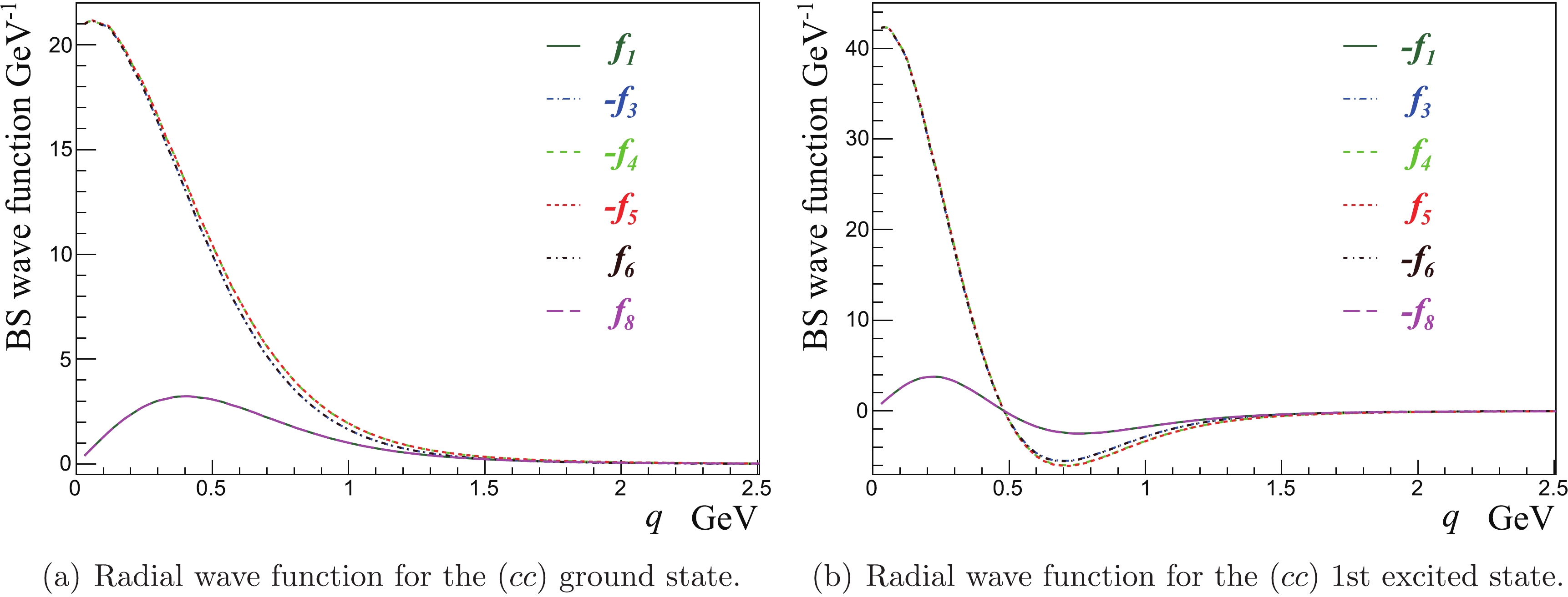
Figure 2. (color online) Radial wave functions of the
$(cc)$ diquark core with$J^P=1^+$ .The wave functions of the diquark cores at the origin are very useful in many applications, and are defined as
$ \psi(\vec x)\mid_{\vec x = \vec 0} = \int \frac{{\rm{d}}^3 \vec s}{(2\pi)^3} \varphi^c(p,s_\perp) \equiv \psi_{\rm{V}}{\not \!\!{\text{e}}}+\psi_{\rm{T}} {\not \!\!{\text{e}}} \hat{\not \!\!p}, $

(15) where
$ \psi_{\rm{V}} $ and$ \psi_{\rm{T}} $ are related to the Salpeter radial wave functions by$ \notag \begin{aligned} \psi_{\rm{V}} & = -\frac{1}{4}\int \frac{{\rm{d}}^3 \vec s}{(2\pi)^3} {\rm{Tr}}\; \varphi^c(|\vec s |) \not \!\!{\text{e}} = -\frac{1}{3}\int \frac{{\rm{d}}^3 \vec s}{(2\pi)^3}(f_3+2f_5),\\ \psi_{\rm{T}} & = -\frac{1}{4 }\int \frac{{\rm{d}}^3 \vec s}{(2\pi)^3}{\rm{Tr}}\; \varphi^c(|\vec s |) \hat{\not \!\!p}\not \!\!{\text{e}} = +\frac{1}{3}\int \frac{{\rm{d}}^3 \vec s}{(2\pi)^3}(f_4-2f_6) . \end{aligned} $

The obtained numerical values of
$ \psi_{\rm{V}} $ and$ \psi_{\rm{T}} $ are listed in Table 2.diquark cores $(cc)$ 

$(bc)$ 

$(bb)$ 

$\psi_{\rm{V}}$ 

0.155 0.299 0.618 $\psi_{\rm{T}}$ 

−0.144 −0.287 −0.600 Table 2. Wave functions at the origin for the ground states of
$1^+$ diquark cores$(cc)$ ,$(bc)$ and$(bb)$ (in GeV2). -
In BSEs for mesons or diquarks, the constituent quarks (antiquarks) are point-like particles. But in BSEs for baryons in terms of quarks and diquarks, the structure of the non-pointlike diquarks has to be considered. The coupling between diquarks and gluons is modified by the form factor. Thus, we discuss in this subsection the relevant form factors in the Mandelstam formulation.
The Feynman diagrams of the doubly heavy diquark core coupling to a gluon are shown in Fig. 3. Since the coupling vertex
$ \Sigma^{\alpha\beta\mu} $ is conserved as the ‘vector current matrix element’, it can be decomposed into three independent form factors$ \sigma_i (i = 1,3,5) $ as
Figure 3. (color online) The vertex diagram of the diquark core coupling to a gluon.
$ \begin{split} {\displaystyle\Sigma ^{\alpha \beta \mu }} = & - {\sigma _1}({t^2}){g^{\alpha \beta }}{(p + p')^\mu } + {\sigma _3}({t^2})({p^\beta }{g^{\alpha \mu }} + {{p'}^\alpha }{g^{\beta \mu }}) \hfill \\ & + {\sigma _5}({t^2}){{p'}^\alpha }{p^\beta }({p^\mu } + {{p'}^\mu }), \hfill \\ \end{split} $

where
$ \sigma_i $ only depend on the transfer momentum$ t^2 \equiv (p-p')^2 $ . Note that in the instantaneous approximation,$ p^0 = p'^0 $ and hence$ t^2 = (p_\perp-p'_\perp)^2 $ is always space-like. Considering that the contributions of$ \sigma_3 $ and$ \sigma_5 $ to BSEs of baryons is small compared with$ \sigma_1 $ , we keep the dominant$ \sigma_1 $ only, and omit the subscript for simplicity.In view of the Feynman diagrams in Fig. 3, the form factor consists of two terms
$ \begin{aligned} \Sigma^{\alpha\beta\mu}& = \frac{1}{2}\left(\Sigma^{\alpha\beta\mu}_1+\Sigma^{\alpha\beta\mu}_2 \right), \end{aligned} $

(16) where the factor
$ \frac{1}{2} $ is due to the normalization condition, and guarantees that the form factor$ \sigma(t^2) = 1 $ at zero transfer momentum ($ t^2 = 0 $ ). Explicitly, for example, the amplitude$ \Sigma^{\alpha\beta\mu}_1 $ corresponding to Fig. 3(a) reads$ \notag \begin{split} \Sigma^{\alpha\beta\mu}_1 = &-\int \frac{{\rm{d}}^4 s}{(2\pi)^4} {\rm{Tr}}\; \bar{\Gamma}^\beta_c(p',s') S(s_1)\Gamma^\alpha_c(p,s) S(-s_2) \gamma^\mu S(-s'_2)\\ &\simeq \int \frac{{\rm{d}}^3 \vec s}{(2\pi)^3} {\rm{Tr}}\; \bar{\varphi}^\beta_c(p',s'_{\!\perp})\gamma^0 \varphi^\alpha_c(k_1,s_\perp) \gamma^\mu , \end{split} $

where the contour integration over
$ s^0 $ is performed and only the dominant contribution is kept. The amplitude of Fig. 3(b) can be easily obtained from the relation$ \Sigma^{\alpha\beta\mu}_2 = \Sigma^{\alpha\beta\mu}_1 $ with$ (\mu_1\rightleftharpoons \mu_2) $ .Inserting the
$ 1^+ $ Salpeter wave function Eq. (12) into Eq. (16), we obtain$ \sigma $ for$ 1^+ $ $ (cc) $ diquark in the ground and first excited states, which are shown in Fig. 4. For convenience, we parameterize the obtained numerical form factor$ \sigma $ as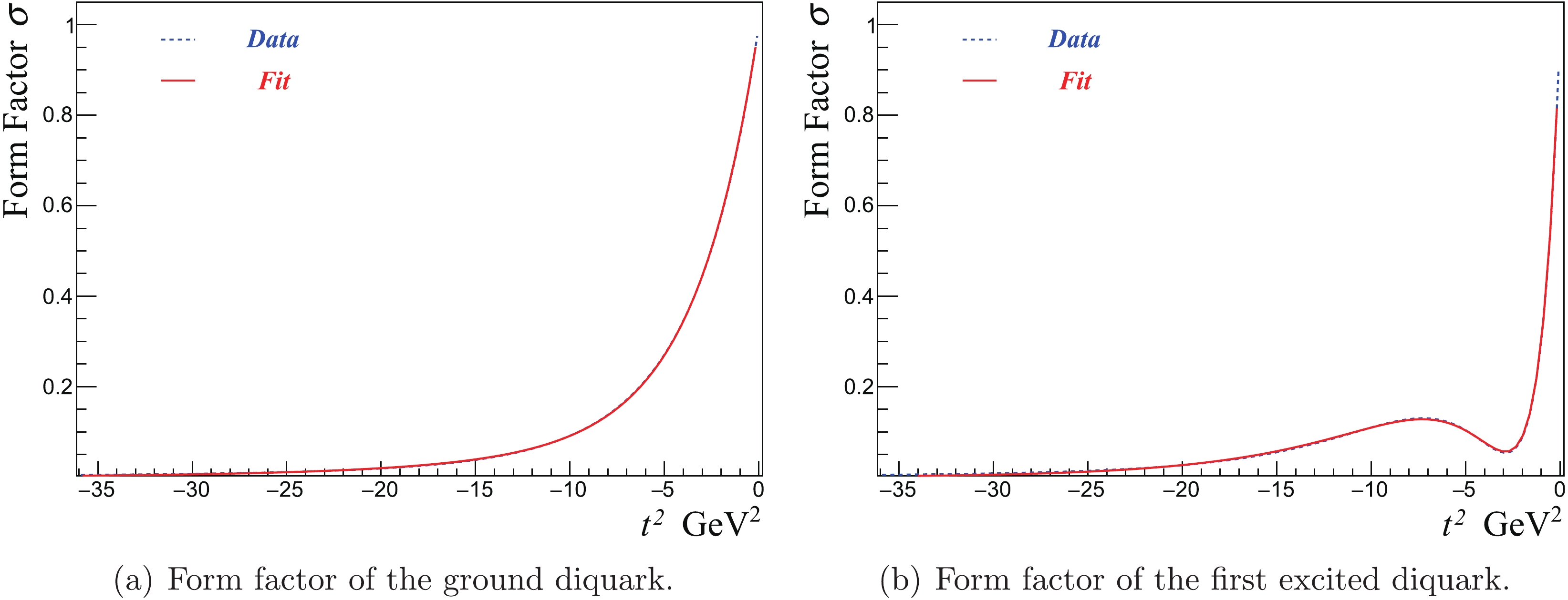
Figure 4. (color online) Form factor of the
$1^+$ $(cc)$ diquark core coupling to a gluon.$ \sigma(t^2) = Ae^{\kappa_1t^2}+(1-A)e^{\kappa_2t^2} . $

(17) For example, we obtain
$ A = 0.162, \; \kappa_1 = 0.109, \; \kappa_2 = 0.312 $ for the ground state. -
In this section, we first construct the Bethe-Salpeter equation of the
$ 1^+ $ diquark core and a light quark, and then derive the three-dimensional (Bethe-)Salpeter equation in the instantaneous approximation. Finally, we compute the mass spectra and wave functions for baryons with the quantum numbers$ J^P = \frac{1}{2}^+ $ and$ \frac{3}{2}^+ $ . -
The BS equation for a baryon with the
$ 1^+ $ heavy diquark core is schematically depicted in Fig. 5, which can be expressed using the matrix notation as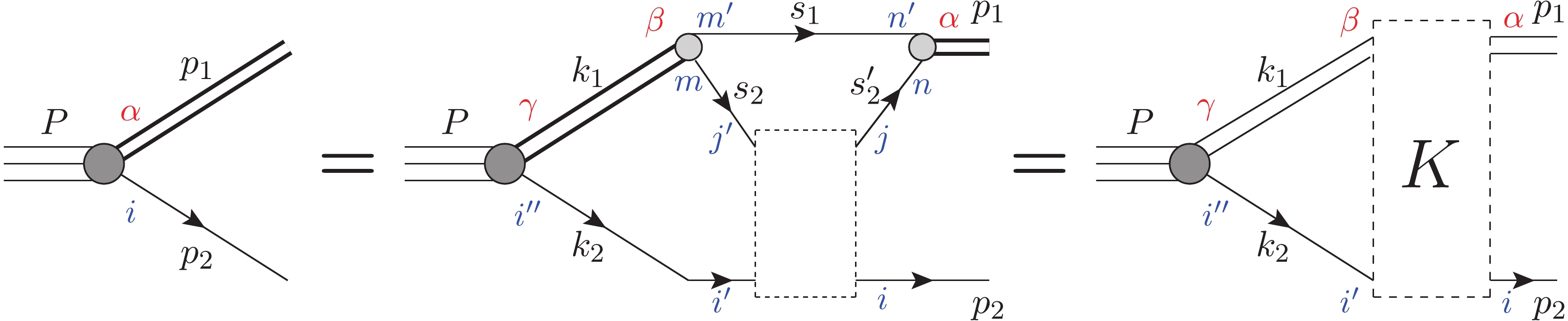
Figure 5. (color online) The Bethe-Salpeter equation for a baryon based on the diquark model. The Greek (red) letters are the Lorentz indices; the Roman (blue) letters are the Dirac indices.
$P, p_1(k_1),p_2(k_2)$ denote the momenta of the baryon, heavy diquark and the third light quark, respectively.$\begin{split} {\Gamma ^\alpha }(P,q,r) =& \int {\frac{{{{\text{d}}^4}k}}{{{{(2\pi )}^4}}}} ( - i){K^{\alpha \beta }}({p_1},{k_1};{p_2},{k_2}) \hfill \\ &\times\left[ {S({k_2}){\Gamma ^\gamma }(P,k,r){D_{\beta \gamma }}({k_1})} \right], \hfill \\ \end{split} $

(18) where
$ \Gamma^\alpha(P,q,r) $ is the BS vertex of the baryon;$ P $ is the baryon momentum with$ P^2 = M^2 $ , and$ M $ the baryon mass;$ r $ is the baryon spin state;$ (-i)K(p_1,k_1;p_2,k_2) $ represents the effective diquark-quark interaction kernel; and$ D_{\beta\gamma}(k_1) = i\frac{-g^{\beta\gamma}+ p^\beta_1p^\gamma_1/m_1^2}{p_1^2-m_1^2+i\epsilon} $ is the free diquark propagator (axial-vector particle) with mass$ m_1 $ . We do not consider here the self-energy correction of the doubly heavy diquark. The internal momenta$ q $ and$ k $ are defined as$ q = \alpha_2 p_1-\alpha_2 p_2,\; \; \; \; k = \alpha_2 k_1-\alpha_1 k_2, $

where
$ \alpha_i = \frac{m_i}{m_1+m_2} $ , and$ m_2 $ represents the constituent mass of the third quark. In the following, the symbols$ P $ and$ r $ in the BS vertex$ \Gamma^\alpha(P,q,r) $ are omitted unless it is necessary.In terms of the diquark form factor, the baryon effective interaction kernel can be simply expressed as
$ (-i)K^{\alpha\beta}(p_1,k_1;p_2,k_2) = - iV_{\rm{M}}(k-q)\Sigma^{\alpha\beta\mu} \gamma_\mu. $

(19) In principle, the form factors must be calculated for off-shell diquarks. In this work, we simply generalize the on-shell form factors obtained in the previous section to the off-shell ones, namely,
$ \Sigma^{\alpha\beta\mu} = \sigma(t^2) g^{\alpha\beta}h^\mu $ and$ h = k_1+p_1 $ . Note that the diquark-quark potential is now modified by the form factor, which reflects the structure effect of the non-pointlike diquark.The BS wave function
$ B_\alpha(P,q) $ of the baryon can be defined as$ B_\alpha(P,q) = S(p_2) D_{\alpha\beta}(p_1) \Gamma^{\beta}(P,q), $

(20) with the constraint condition
$ P^\alpha B_{\alpha}(P,q) = 0 $ . Accordingly, the normalization condition can be expressed as,$ -\!i\int \int \frac{{\rm{d}}^4 q}{(2\pi)^4}\frac{{\rm{d}}^4 k}{(2\pi)^4} \; \bar{B}_\alpha(q,\bar r) \frac{\partial}{\partial P^0}\!\! \left[ I^{\alpha\beta}(P,k,q) \right] B_\beta(k,r) \!=\! 2M \delta_{r\bar r}, $

(21) where the operator
$ I^{\alpha\beta}(P,k,q) $ has the following form,$\begin{split} {I^{\alpha \beta }}(P,k,q) =& {S^{ - 1}}({p_2})D_{\alpha \beta }^{ - 1}({p_1}){(2\pi )^2}{\delta ^4}(k - q) \hfill \\ &+ i{K^{\alpha \beta }}({p_1},{k_1};{p_2},{k_2}). \hfill \\ \end{split} $

(22) -
In the instantaneous approximation, the factor
$ h^0 = 2(\alpha_1M+q_P) $ explicitly depends on$ q_P $ and$ M $ , which is different from the case of mesons or diquarks. As we will see, the factor$ h^0 $ plays an important role in the derivation of the three-dimensional Salpeter equation for baryons. First, we introduce the instantaneous baryon kernel as$ \notag K(k_\perp-q_\perp) = \sigma(t^2) V_{\rm{M}}(k_\perp-q_\perp) \gamma_0 , $

so that we have
$ K^{\alpha\beta}(p_1,k_1) = h^0 g^{\alpha\beta} K(q_\perp-k_\perp) $ . We now define the baryon Salpeter wave function as$ \notag \varphi_\alpha(q_\perp) \equiv -i\int \frac{{\rm d} q_P}{2\pi} B_\alpha(q), $

with the constraint condition
$ P^\alpha \varphi_\alpha = 0 $ .The baryon BS wave function can be expressed as
$ B^\alpha(q) = h^0 S(p_2) D^{\alpha\beta}(p_1) \Gamma_\beta (q_\perp) , $

(23) where the three-dimensional vertex
$ \Gamma_a(q_\perp) $ is expressed by the Salpeter wave function as$ \Gamma_{\alpha} (q_\perp) \equiv \int \frac{{\rm{d}}^3 k_\perp}{(2\pi)^3}K(k_\perp-q_\perp) \varphi_\alpha(k_\perp). $

(24) Due to the constraint condition
$ P_\alpha \varphi^\alpha(P) = 0 $ , the components of$ D^{\alpha\beta}(p_1) $ parallel to$ P $ vanish. Hence, we can rewrite$ D^{\alpha\beta}(p_1) $ as$ \notag D^{\alpha\beta}(p_1) = i\frac{\vartheta^{\alpha\beta}}{p_1^2-m_1^2+i\epsilon},\; \; \; \vartheta^{\alpha\beta}\equiv -g^{\alpha\beta}+\frac{p_{1\perp}^\alpha p_{1\perp}^\beta}{m_1^2}. $

Note that in Ref. [27], the term
$ i\frac{p^\alpha_1 p^\beta_1/m_1^2}{p_1^2-m_1^2} $ is simply neglected.We follow Salpeter's method from Ref. [64]. Performing the contour integral over
$ q_P $ on both sides of Eq. (23) (see Appendix A.2 for details), we finally obtain the Schrödinger-type Salpeter equation for baryons with$ 1^+ $ diquark cores as$ M\varphi^\alpha(q_\perp) = ( \omega_1+ \omega_2)\hat H( p_{2\perp})\varphi^\alpha(q_\perp) + \hat{H}(p_{2\perp}) \gamma^0 \vartheta^{\alpha\beta}\Gamma_\beta (q_\perp) , $

(25) where the baryon mass
$ M $ behaves as the eigenvalue. The first term expresses the contribution of the kinetic energy, and the second term of the potential energy. The normalization condition can be expressed as (see Appendix A.3 for details)$ \begin{split} \int {\frac{{{{\text{d}}^3}{q_ \bot }}}{{{{(2\pi )}^3}}}} {{\bar \varphi }_\alpha }&(P,{q_ \bot },\bar r){\gamma ^0}2\left( {{\alpha _1}M\hat H({p_{2 \bot }}) + {\omega _q}} \right) \hfill \\ &\times{d^{\alpha \beta }}{\varphi _\beta }(P,{q_ \bot },r) = 2M{\delta _{r\bar r}}, \hfill \\ \end{split} $

(26) with
$ \omega_q\equiv \alpha_2 \omega_1-\alpha_1 \omega_2 $ and$ d^{\alpha\beta}\equiv-g^{\alpha\beta}-\frac{p^\alpha_{1\perp} p^\alpha_{1\perp}}{ \omega_1^2} $ . -
In this subsection, we construct the baryon wave functions directly from the good quantum number
$ J^P $ . The$ D $ -wave components are then automatically included and the possible S-D mixing can also be obtained directly by solving the corresponding BSE.For ground states with
$ L = 0 $ , where$ L $ denotes the diquark-quark orbital angular momentum, the$ 1^+ $ diquark and the$ \frac{1}{2}^+ $ quark can form a baryon doublet$ (\frac{1}{2},\frac{3}{2})^+ $ . The wave function of$ J^P = \frac{1}{2}^+ $ baryon, analyzing its total angular momentum and the Lorentz and Dirac structures, can be decomposed it as$\begin{split} {\varphi _\alpha }(P,{q_ \bot },r) = &\left( {{g_1} + {g_2}\frac{{{{\not\!\! q}_ \bot }}}{q}} \right){\xi _{1\alpha }}{\gamma ^5}u(P,r) \hfill \\ &+ \left( {{g_3} + {g_4}\frac{{{{\not \!\!q}_ \bot }}}{q}} \right){{\hat q}_{ \bot \alpha }}{\gamma ^5}u(P,r) = {A_\alpha }u(P,r), \hfill \\ \end{split} $

(27) where we defined
$ A_\alpha $ so as to factor out the spinor;$ \xi_{1\alpha} = (\gamma_\alpha+\frac{P_\alpha}{M}) $ , and$ q = \sqrt{-q_\perp^2} $ ; the radial wave functions$ g_i\; (i = 1,2,3,4) $ explicitly depend on$ q $ ;$ u(P,r) $ is the Dirac spinor with momentum$ P $ and spin state$ r $ . The conjugation is defined as usual$ \bar \varphi_\alpha(P,q_\perp,r) = \varphi_\alpha^\dagger \gamma_0 $ . Note that in Ref. [34] only$ g_1 $ and$ g_2 $ are included. In fact, the full Salpeter wave function should have four independent terms. The ‘small components’$ g_3 $ and$ g_4 $ correspond respectively to the$ P $ - and$ D $ -wave components, and play a certain role in the exact solutions for$ J^P = \frac{1}{2}^+ $ baryons. In particular, they are important for the excited states. To see the partial-wave components clearly, we rewrite the Salpeter wave function of$ \frac{1}{2}^+ $ baryon in terms of the spherical harmonics,$\begin{split} {\varphi _\alpha } = &{C_0}Y_0^0\left( {{g_1}{\xi _{1\alpha }} - {g_4}\frac{{{\gamma _\alpha }}}{3}} \right){\gamma ^5}u + {C_1}\left( {Y_1^0{\Gamma _{\alpha 3}} - Y_1^{ - 1}{\Gamma _{\alpha + }} - Y_1^1{\Gamma _{\alpha - }}} \right) \hfill \\ &\times {\gamma ^5}u + {C_2}{g_4}\left[ {Y_2^{ - 2}{g_{\alpha + }}{\gamma _ + } - Y_2^{ - 1}\frac{{({g_{\alpha 3}}{\gamma _ + } + {g_{\alpha + }}{\gamma _3})}}{{\sqrt 2 }}} \right. \hfill \\ & + Y_2^0\frac{{({g_{\alpha + }}{\gamma _ - } + {g_{\alpha - }}{\gamma _ + } + 2{g_{\alpha 3}}{\gamma _3})}}{{\sqrt 6 }} \hfill \\ &\left. { - Y_2^1\frac{{({g_{\alpha 3}}{\gamma _ - } + {g_{\alpha - }}{\gamma _3})}}{{\sqrt 2 }} + Y_2^2{g_{\alpha - }}{\gamma _ - }} \right]{\gamma ^5}u, \hfill \\ \end{split} $

(28) where the coefficients are
$ C_0 = 2\sqrt{ \pi} $ ,$ C_1 = \frac{1}{\sqrt{3}}C_0 $ , and$ C_2 = \sqrt{\frac{2}{15}}C_0 $ ;$ \gamma_{\pm} = \mp\frac{1}{\sqrt{2}} (\gamma_1\pm i \gamma_2) $ ;$ \Gamma_{\alpha{\pm}} = \mp \frac{1}{\sqrt{2}}(\Gamma_{\alpha1}\pm i \Gamma_{\alpha2}) $ , and$ \Gamma_{\alpha i} \equiv (g_2 \gamma_i \xi_{1\alpha} + g_3 g_{\alpha i}) $ with$ i = 1,2,3{\text{;}} g_{\alpha\pm} = \mp$ $ \frac{1}{\sqrt{2}} \left(g_{\alpha1}\pm \right.$ $\left. i g_{\alpha2}\right) $ , where$ g_{\alpha\beta} $ denotes the Minkowski metric tensor;$ Y_l^m $ are the usual spherical harmonics.From the above decomposition Eq. (28), we conclude that the Salpeter wave function of
$ \frac{1}{2}^+ $ baryon contains the$ S $ -,$ P $ -, and$ D $ -wave components. The$ g_1 $ part corresponds to the$ S $ -wave;$ g_{2} $ and$ g_3 $ parts correspond to the$ P $ -wave; and$ g_4 $ contributes to both the$ S $ - and$ D $ -wave components. The numerical details are presented in the next section.With the wave function of Eq. (27), the Salpeter equation Eq. (25) can be expressed as
$ \begin{split} M{A_\alpha }u(P,r) = &({\omega _1} + {\omega _2})\hat H({p_{2 \bot }}){A_\alpha }u(P,r) + {\vartheta _{\alpha \beta }}\hat H({p_{2 \bot }}){\gamma ^0} \hfill \\ &\times\int {\frac{{{{\text{d}}^3}{k_ \bot }}}{{{{(2\pi )}^3}}}} K({k_ \bot } - {q_ \bot }){A^\beta }u(P,r). \hfill \\ \end{split} $

(29) Projecting out the radial wave functions, we get four coupled eigenvalue equations. The details are presented in Appendix A.4. Solving the equations numerically, the mass spectra and radial wave functions can be obtained. The normalization condition Eq. (26) can be expressed in terms of the radial wave functions as
$\begin{split} \int {\frac{{{{\text{d}}^3}{q_ \bot }}}{{{{(2\pi )}^3}}}} &\left[ {2\left( {{\omega _q} + {\alpha _1}M\frac{{{m_2}}}{{{\omega _2}}}} \right)(3{c_3}g_1^2 - 2{c_1}{g_1}{g_4} + {c_1}g_4^2)} \right. \hfill \\ &+ 2\left( {{\omega _q} - {\alpha _1}M\frac{{{m_2}}}{{{\omega _2}}}} \right)(2{c_1}{g_2}{g_3} + {c_1}g_3^2 + 3{c_3}g_2^2) \hfill \\ & \left. { + 4{\alpha _1}M\frac{q}{{{\omega _2}}}({c_1}{g_2}{g_4} \!+\! {c_1}{g_3}{g_4} \!-\! {c_1}{g_1}{g_3}\! - \!3{c_3}{g_1}{g_2})} \right] \!=\! 1, \hfill \\ \end{split} $

where
$ c_1 = 1-\frac{\vec q ^2}{ \omega_1^2} $ and$ c_3 = 1-\frac{\vec q ^2}{3 \omega_1^2} $ , and the spinor summation$ \sum_r u(r)\bar u(r) = {\not\!\! P}+M $ is used.Similarly, the Salpeter wave function for
$ J^P = \frac{3}{2}^+ $ baryons can be constructed using the Rarita-Schwinger spinor$ u_\alpha(P,r) $ as$\begin{split} {\varphi _\alpha }(P,{q_ \bot },r) =& \left( {{t_1} + {t_2}\frac{{{{\not \!\!q}_ \bot }}}{q}} \right){u_\alpha }(P,r) + \left( {{t_3} + {t_4}\frac{{{{\not \!\!q}_ \bot }}}{q}} \right){\xi _{3\alpha }}(P){u_{{{\hat q}_ \bot }}}(P,r) \hfill \\ & + \left( {{t_5} + {t_6}\frac{{{{\not\!\! q}_ \bot }}}{q}} \right){{\hat q}_{ \bot \alpha }}{u_{{{\hat q}_ \bot }}}(P,r) = {A_{\alpha \beta }}{u^\beta }(P,r), \hfill \\ \end{split} $

(30) where we define the tensor
$ A_{\alpha\beta} $ for later convenience;$ \xi_{3\alpha}(P) = (\gamma_\alpha-\frac{ P_\alpha}{M}) $ ; and$ t_i\; (i = 1,\cdots,6) $ are the radial wave functions depending on$ q $ . According to the Rarita-Schwinger equation, we have$ P_\alpha \varphi^\alpha = 0 $ . Note that the full Salpeter wave function has six independent terms, while in Ref. [34] only the first two,$ t_1 $ and$ t_2 $ , are considered. The decomposition in terms of spherical harmonics is similar to the case of$ J^P = \frac{1}{2}^+ $ and we do not repeat it here. It is evident that$ t_{3} $ ,$ t_4 $ ,$ t_5 $ , and$ t_6 $ correspond to the$ P $ ,$ ^2D $ ,$ ^4D $ , and$ F $ partial waves, respectively. This means that only the largest$ S $ -wave and part of the$ P $ -wave components are considered. Note that the$ D(F) $ -wave is always mixed with the$ S(P) $ -wave components, i.e.$ t_{4(5)} $ always contribute to the$ S $ -wave besides the$ D $ -wave, while$ t_6 $ contributes to the$ P $ -wave and the$ F $ -wave. Further analysis of their importance is presented later.We now obtain the following mass eigenvalue equation
$ \begin{split} M{A_{\alpha \beta }}{u^\beta }(P,r) =& ({\omega _1} + {\omega _2})\hat H({p_{2 \bot }}){A_{\alpha \beta }}{u^\beta }(P,r) \hfill \\ & \!\!\!+ {\vartheta _{\alpha \beta }}\hat H({p_{2 \bot }}){\gamma ^0}\int {\frac{{{{\text{d}}^3}{k_ \bot }}}{{{{(2\pi )}^3}}}} K({k_ \bot } \!- \!{q_ \bot }){A^{\beta \gamma }}{u_\gamma }(P,r), \hfill \\ \end{split} $

(31) which is equivalent to six coupled eigenvalue equations, similar to the
$ \frac{1}{2}^+ $ case, and we again omit the details. The normalization condition can be written as$\begin{split} \int& {\frac{{{{\text{d}}^3}{q_ \bot }}}{{{{(2\pi )}^3}}}} \frac{2}{3}\left\{ {\left[ {3{c_3}(t_1^2 + t_4^2) - 4{c_2}{t_1}{t_4} - 2{c_1}({t_1}{t_5} - {t_4}{t_5}) + {c_1}t_5^2} \right]} \right. \hfill \\ &\times \left( {{\omega _q} + {\alpha _1}M\frac{{{m_2}}}{{{\omega _2}}}} \right) + \left[ {3{c_3}(t_2^2 + t_3^2) + 4{c_2}{t_2}{t_3} - 2{c_1}({t_2}{t_6} + {t_3}{t_6})} \right. \hfill \\ & \left. { + {c_1}t_6^2} \right]\left( {{\omega _q} - {\alpha _1}M\frac{{{m_2}}}{{{\omega _2}}}} \right) - 2{\alpha _1}M\frac{q}{{{\omega _2}}}\left[ {3{c_3}({t_1}{t_2} - {t_3}{t_4})} \right. \hfill \\ &{\left. { + 2{c_2}({t_1}{t_3} - {t_2}{t_4}) - {c_1}({t_1}{t_6} + {t_2}{t_5} + {t_3}{t_5} - {t_4}{t_6} - {t_5}{t_6})} \right]} \Big\} = 1, \hfill \\ \end{split} $

where
$ c_2 = 1-\frac{\vec q ^2}{2 \omega_1^2} $ , and the following completeness relation of the Rarita-Schwinger spinor [65] was used:$ \begin{split} {u^\alpha }(P,r){{\bar u}^\beta }(P,r) =& (\not\!\! P + M)\left[ { - {g^{\alpha \beta }} + \frac{1}{3}{\gamma ^\alpha }{\gamma ^\beta }} \right. \hfill \\ & \left. { - \frac{{{P^\alpha }{\gamma ^\beta } - {P^\beta }{\gamma ^\alpha }}}{{3M}} + \frac{{2{P^\alpha }{P^\beta }}}{{3{M^2}}}} \right]. \hfill \\ \end{split} $

-
To solve the Salpeter equation for baryons, we need to specify the parameter
$ V_0 $ in the potential for the diquark core and the light quark. Unlike the doubly heavy mesons, the experimental data for the doubly heavy baryons is very limited. Hence, we cannot fix$ V_0 $ by fitting the experimental data. We compute$ V_0 $ by taking the spin-weighted average of$ V_0 $ of the corresponding mesons (see details in Appendix A.5). The fixed values of$ V_0 $ are listed in Table 3. Note that all parameters in the model are now fixed by the meson sector.$\frac{1}{2}^+$ baryons

$\Xi_{cc}^{++}$ 

$\Xi_{cc}^+$ 

$\Omega^+_{cc}$ 

$\Xi_{cb}^{+}$ 

$\Xi_{cb}$ 

$\Omega_{cb}$ 

$\Xi_{bb}$ 

$\Omega_{bb}^-$ 

$-V_0$ 

$0.478$ 

$0.476$ 

$0.454$ 

$0.404$ 

$0.403$ 

$0.382$ 

$0.330$ 

$0.310$ 

$\frac{3}{2}^+$ baryons

$\Xi_{cc}^{*++}$ 

$\Xi_{cc}^{*+}$ 

$\Omega^*_{cc}$ 

$\Xi_{cb}^{*+}$ 

$\Xi^{*0}_{cb}$ 

$\Omega^*_{cb}$ 

$\Xi^*_{bb}$ 

$\Omega_{bb}^{*-}$ 

$-V_0$ 

$0.378$ 

$0.376$ 

$0.352$ 

$0.337$ 

$0.336$ 

$0.313$ 

$0.296$ 

$0.275$ 

Table 3. The parameter
$(-V_0)$ (in GeV) determined by the spin-weighted average method.In this work, we calculate
$ \Xi^{(*)}_{cc} $ ,$ \Omega^{(*)}_{cc} $ ,$ \Xi^{(*)}_{cb} $ ,$ \Omega^{(*)}_{cb} $ ,$ \Xi^{(*)}_{bb} $ , and$ \Omega^{(*)}_{bb} $ for the$ J^P = \frac{1}{2}^+(\frac{3}{2}^+) $ doubly heavy baryons. In the relativistic Bethe-Salpeter equation approach, the total angular momentum$ J $ and the space parity$ P $ of baryons are good quantum numbers. To reflect the dominant properties, we label the baryon states by the nonrelativistic notation as$ n_{\rm{B}}{^{2s_{\rm{B}}+1}L_{J}}(n_{\rm{D}}L_{\rm{D}}) $ :$ n_{\rm{D}} $ denotes the radial quantum number of the heavy diquark core;$ L_{\rm{D}} $ the orbital angular momentum of the diquark;$ n_{\rm{B}} $ the radial quantum number of the baryon;$ L $ the quantum number of the diquark-quark orbital angular momentum;$ (2s_{\rm{B}}+1) $ the multiplicity of the baryon spin$ s_{\rm{B}} $ ; and$ J $ the total angular momentum of the baryon. Consequently,$ \frac{1}{2}^+ $ baryons can have states$ {^2S_{1/2}} $ or$ {^4D_{1/2}} $ , or their mixing, and$ \frac{3}{2}^+ $ baryons$ {^4S_{3/2}} $ ,$ {^4D_{3/2}} $ ,$ {^2D_{3/2}} $ , or their mixing.The mass spectra of the
$ J^P = \frac{1}{2}^+ $ doubly heavy baryons with flavors$ (ccq) $ ,$ (bcq) $ and$ (bbq) $ are presented in Table 4, including the diquark cores in the excited$ 2S $ and$ 1D $ states. Note that the baryon masses of the$ 1^2S_{1/2}(1D) $ and$ 1^4D_{1/2}(1S) $ states are comparable, namely, the different$ D $ -wave orbital angular momenta contribute similarly to the total baryon mass. The wave functions of$ \Xi_{cc}^{++} $ , as an example, are presented in Fig. 6. From the figure, one may clearly see the correspondence of the radial quantum number$ n_{\rm{B}} $ and the node number of the wave function:$ g_{1} $ and$ g_{4} $ correspond to the$ ^2 S $ and$ ^4 D $ partial wave components, respectively, and$ g_2 $ and$ g_3 $ represent the small$ P $ -wave components with different radial numbers. Comparing the weights of the partial wave components, one can see that the ground state$ n = 1 $ is dominated by the$ S $ -wave and has a negligible$ D $ -wave, whereas the excited states$ n = 2,3,4\cdots $ have sizable$ D $ -wave components. This means that ignoring the components$ g_{3,4} $ in the excited states would destroy the results. Therefore, as mentioned in the previous section, the full structure of the wave functions must be considered.$n$ 

$n_{\rm{B}}{^{2s_{\rm{B}}+1}L_J}(n_{\rm{D}}L_{\rm{D}})$ 

$\Xi_{cc}^{++}$ 

$\Xi_{cc}^+$ 

$\Omega^+_{cc}$ 

$\Xi_{cb}^{+}$ 

$\Xi_{cb}$ 

$\Omega_{cb}$ 

$\Xi_{bb}$ 

$\Xi_{bb}^-$ 

$\Omega_{bb}^-$ 

1 $1^2S_{1/2}(1S)$ 

$ 3601^{-28}_{+28}$ 

$ 3606^{-28}_{+28}$ 

$ 3710^{-28}_{+27}$ 

$ 6931^{-28}_{+27}$ 

$ 6934^{-28}_{+27}$ 

$ 7033^{-26}_{+24}$ 

$10182^{-25}_{+25}$ 

$10184^{-25}_{+25}$ 

$10276^{-23}_{+22}$ 

2 $2^2S_{1/2}(1S)$ 

$4122^{-38}_{+38}$ 

$4128^{-40}_{+38}$ 

$4247^{-38}_{+38}$ 

$7446^{-37}_{+38}$ 

$7450^{-39}_{+38}$ 

$7560^{-36}_{+35}$ 

$10708^{-35}_{+35}$ 

$10710^{-36}_{+34}$ 

$10816^{-34}_{+32}$ 

3 $1^4D_{1/2}(1S)$ 

$4151^{-38}_{+39}$ 

$4157^{-38}_{+38}$ 

$4289^{-37}_{+36}$ 

$7463^{-35}_{+35}$ 

$7467^{-34}_{+35}$ 

$7598^{-33}_{+33}$ 

$10732^{-32}_{+33}$ 

$10735^{-32}_{+33}$ 

$10863^{-32}_{+32}$ 

4 $3^2S_{1/2}(1S)$ 

$4504^{-54}_{+54}$ 

$4510^{-54}_{+54}$ 

$4632^{-53}_{+52}$ 

$7818^{-51}_{+52}$ 

$7822^{-52}_{+51}$ 

$7935^{-49}_{+50}$ 

$11084^{-49}_{+48}$ 

$11086^{-50}_{+48}$ 

$11196^{-48}_{+47}$ 

1 $1^2S_{1/2}(2S)$ 

$4136^{-36}_{+35}$ 

$4141^{-35}_{+35}$ 

$4261^{-33}_{+33}$ 

$7417^{-32}_{+32}$ 

$7420^{-33}_{+33}$ 

$7531^{-30}_{+32}$ 

$10618^{-30}_{+28}$ 

$10620^{-29}_{+28}$ 

$10724^{-28}_{+26}$ 

1 $1^2S_{1/2}(1D)$ 

$4140^{-33}_{+33}$ 

$4145^{-33}_{+33}$ 

$4262^{-32}_{+32}$ 

$7438^{-32}_{+31}$ 

$7441^{-32}_{+31}$ 

$7550^{-30}_{+30}$ 

$10660^{-28}_{+28}$ 

$10661^{-28}_{+28}$ 

$10763^{-26}_{+26}$ 

Table 4. Mass spectra of the
$J^P=\frac{1}{2}^+$ doubly heavy baryons, in units of MeV. Symbols used to label the baryon states are:$n_{\rm{D}}$ denotes the radial quantum number of the doubly heavy diquark core inside the baryon;$L_{\rm{D}}$ the orbital angular momentum of the diquark;$n_{\rm{B}}$ the radial number of the baryon;$(2s_{\rm{B}}+1)$ the baryon spin multiplicity;$L$ the orbital angular momentum quantum number between the diquark core and the light quark; and finally$J$ the total baryon angular momentum.
Figure 6. (color online) BS radial wave functions of
$\Xi_{cc}^{++}$ with the energy levels$n=1,\cdots,4$ ;$g_{1}$ and$g_{4}$ correspond to the$^2{\rm S}$ and$^4{\rm D}$ components, and$g_{2(3)}$ corresponds to the$P$ -wave;$n_{\rm{B}}$ is the number of the node plus one. Almost every state contains the$S$ -,$P$ - and$D$ -wave components.The mass spectra of the
$ J^P = \frac{3}{2}^+ $ doubly heavy baryons are presented in Table 5, and the radial wave functions of$ \Xi_{cc}^* $ are shown in Fig. 7 as an example.$ J^P = \frac{3}{2}^+ $ baryons, besides the$ {^{4}S_{3/2}} $ partial waves, also contain two different$ D $ -waves,$ {^4 D_{3/2}} $ and$ {^2D_{3/2}} $ , which belong to the quartet$ (\frac{7}{2},\frac{5}{2},\frac{3}{2},\frac{1}{2})^+ $ and the doublet$ (\frac{5}{2},\frac{3}{2})^+ $ , respectively. The baryon masses with excited$ 2S $ and$ 1D $ diquarks are listed in the last two rows. Note that the masses of the$ 1^4S_{3/2}(1D) $ states are close to the$ 1^2D_{3/2}(1S) $ states, but are much lower than the masses of the$ 1^4D_{3/2}(1S) $ states. Similar analysis of the wave functions shows that almost every state contains all possible$ S $ -,$ P $ -,$ D $ - and$ F $ -wave components. The analysis of the weight of the partial waves suggests that the$ n = 1,2 $ states are mainly characterized by the$ 1{^{4}S} $ and$ 2{^{4}S} $ components, with the$ D $ -wave slightly mixed in. However, for the$ n = 3,4 $ states, the$ 1^2D $ and$ 1^4D $ components become dominant. These features again emphasize the importance of using the full structure of the wave functions.$n$ 

$n_{\rm{B}}{^{2s_{\rm{B}}+1}\! L_J}(n_{\rm{D}}L_{\rm{D}})$ 

$\Xi_{cc}^{*++}$ 

$\Xi_{cc}^{*+}$ 

$\Omega^*_{cc}$ 

$\Xi_{cb}^{*+}$ 

$\Xi^*_{cb}$ 

$\Omega^*_{cb}$ 

$\Xi_{bb}^{*}$ 

$\Xi^{*-}_{bb}$ 

$\Omega^{*-}_{bb}$ 

1 $1^4S_{3/2}(1S)$ 

$3703^{-28}_{+28}$ 

$3706^{-28}_{+28}$ 

$3814^{-27}_{+27}$ 

$6997^{-27}_{+27}$ 

$7000^{-27}_{+25}$ 

$7101^{-25}_{+25}$ 

$10214^{-25}_{+25}$ 

$10216^{-24}_{+25}$ 

$10309^{-23}_{+24}$ 

2 $2^4S_{3/2}(1S)$ 

$4232^{-40}_{+40}$ 

$4237^{-41}_{+38}$ 

$4356^{-38}_{+38}$ 

$7512^{-39}_{+36}$ 

$7515^{-38}_{+36}$ 

$7627^{-36}_{+33}$ 

$10738^{-35}_{+35}$ 

$10740^{-35}_{+35}$ 

$10847^{-32}_{+33}$ 

3 $1^2D_{3/2}(1S)$ 

$4252^{-37}_{+36}$ 

$4257^{-37}_{+36}$ 

$4395^{-35}_{+36}$ 

$7531^{-35}_{+33}$ 

$7535^{-36}_{+32}$ 

$7668^{-35}_{+32}$ 

$10766^{-32}_{+32}$ 

$10769^{-32}_{+32}$ 

$10898^{-32}_{+32}$ 

4 $1^4D_{3/2}(1S)$ 

$4421^{-46}_{+45}$ 

$4424^{-46}_{+45}$ 

$4520^{-43}_{+43}$ 

$7699^{-43}_{+40}$ 

$7701^{-43}_{+40}$ 

$7791^{-41}_{+37}$ 

$10941^{-40}_{+38}$ 

$10943^{-39}_{+38}$ 

$11028^{-37}_{+36}$ 

1 $1^4S_{3/2}(2S)$ 

$4237^{-36}_{+35}$ 

$4241^{-35}_{+35}$ 

$4365^{-33}_{+33}$ 

$7484^{-33}_{+32}$ 

$7487^{-33}_{+32}$ 

$7601^{-32}_{+30}$ 

$10651^{-28}_{+28}$ 

$10653^{-30}_{+28}$ 

$10759^{-28}_{+28}$ 

1 $1^4S_{3/2}(1D)$ 

$4241^{-33}_{+33}$ 

$4245^{-33}_{+32}$ 

$4366^{-32}_{+32}$ 

$7504^{-30}_{+31}$ 

$7507^{-30}_{+31}$ 

$7619^{-29}_{+30}$ 

$10693^{-28}_{+28}$ 

$10695^{-28}_{+28}$ 

$10798^{-26}_{+26}$ 

Table 5. Mass spectra (in MeV) of the
$\frac{3}{2}^+$ doubly heavy baryons.
Figure 7. (color online) BS radial wave functions of
$\Xi_{cc}^{*}$ with the energy levels$n=1,\cdots,4$ ;$t_{1}$ ,$t_{4}$ and$t_{5}$ correspond to the$^4{S}$ ,$^2{D}$ and$^4\hspace{-0.1em}D$ components,$t_{2(3)}$ and$t_6$ correspond to the$P$ and$F$ -wave. Almost every baryon state contains all$^4{S}$ ,$^2{D}$ and$^4\hspace{-0.1em}D$ components.To determine the sensitivity of the mass spectra on the model parameters, we calculated the theoretical uncertainties by varying simultaneously the parameters
$ \lambda $ and$ a_{1(2)} $ in the quark-diquark bound potential by ±5%, and then searching the parameter space to find the maximum deviation. The obtained theoretical errors are also listed in Table 4 and Table 5, where the relative errors induced by$ \lambda $ and$ a_{1(2)} $ are about 1%. The dependence on the constituent quark mass is almost linear and was not included in the error analysis.Finally, we give a comparison of the predicted spectra of the ground states obtained in this work and in literature, shown in Table 6. We note that our mass spectra agree well with the lattice QCD calculations in Refs. [21,66,67], especially for
$ \Xi^{(*)}_{cc} $ ,$ \Omega^{*}_{cc} $ ,$ \Omega_{cb} $ , and$ \Omega^{(*)}_{bb} $ . The average error of the predictions in Table 6 with respect to Ref. [21] is about 18 MeV.Baryon This [21] [66,67] [22,68] [9] [69] [70] [71] [72] $\Xi_{cc}$ 

3.601 3.610 − 3.627 3.620 3.612 3.547 3.633 3.606 $\Xi_{cc}^*$ 

3.703 3.692 − 3.690 3.727 3.706 3.719 3.696 3.675 $\Omega_{cc}$ 

3.710 3.738 3.712 3.692 3.778 3.702 3.648 3.732 3.715 $\Omega^*_{cc}$ 

3.814 3.822 3.788 3.756 3.872 3.783 3.770 3.802 3.772 $\Xi_{cb}$ 

6.931 6.959 6.945 6.933 6.933 6.919 6.904 6.948 − $\Xi^*_{cb}$ 

6.997 6.985 6.989 6.969 6.980 6.986 6.936 6.973 − $\Omega_{cb}$ 

7.033 7.032 6.994 6.984 7.088 6.986 6.994 7.047 − $\Omega^*_{cb}$ 

7.101 7.059 7.056 − 7.130 7.046 7.017 7.066 − $\Xi_{bb}$ 

10.182 10.143 − 10.162 10.202 10.197 10.185 10.169 10.138 $\Xi^*_{bb}$ 

10.214 10.178 − 10.184 10.237 10.236 10.216 10.189 10.169 $\Omega_{bb}$ 

10.276 10.273 − 10.208 10.359 10.260 10.271 10.259 10.230 $\Omega_{bb}^*$ 

10.309 10.308 − − 10.389 10.297 10.289 10.268 10.258 Table 6. Comparison of the predictions of the ground state masses (in GeV) of the doubly heavy baryons. The results in the third [21] and forth [66,67] columns are from the lattice QCD calculations. Note that here
$\Xi_{bc}$ ,$\Omega_{bc}$ denote the$\frac{1}{2}^+$ $(bcq)$ baryons with$1^+$ $(bc)$ diquark core. -
In summary, we have built in the diquark core picture a theoretical framework to deal with doubly heavy baryons. In the diquark picture, the three-body problem of the doubly heavy baryons is reduced to two two-body bound problems and then solved by the corresponding BSE in the instantaneous approximation. We obtained the mass spectra and wave functions of the
$ J^P = \frac{1}{2}^+ $ and$ \frac{3}{2}^+ $ doubly heavy baryons with 1+ diquark cores. The predicted mass spectra for the doubly heavy baryons agree with those in literature, especially with the lattice QCD computations. Analyzing the wave functions, we found that$ \frac{1}{2}^+ $ and$ \frac{3}{2}^+ $ baryons, especially their excited states, involve$ P $ - and$ D $ -wave components that are not negligible, and even$ F $ -wave for the latter, which means that the non-relativistic wave functions consisting only of the$ S $ or$ D $ partial waves cannot describe well these baryons. The obtained wave functions can be used to calculate lifetimes, production and decay of doubly heavy baryons, which can be tested in future experiments.We thank Hai-Yang Cheng, Xing-Gang Wu, Xu-Chang Zheng, Tian-Hong Wang and Hui-Feng Fu for the helpful discusses and suggestions.
-
The four coupled eigen equations for the 1+ diquark have the following expressions
$ \tag{A1} \begin{split} \mu f_3(s)& = +\frac{\mu_1+\mu_2}{e_1+e_2}(e_1+e_2+V^c_1)f_4(s)+\int \frac{{\rm{d}}^3 \vec u}{2e_1e_2}V^c_2\left[ A_{12}(s,u)f_4(u)+A_{14}(s,u)f_6(u) \right],\\ \mu f_4(s)& = +\frac{e_1+e_2}{\mu_1+\mu_2}(e_1+e_2+V^c_1)f_3(s)+\int \frac{{\rm{d}}^3 \vec u}{2e_1e_2}V^c_2\left[ A_{21}(s,u)f_3(u)+A_{23}(s,u)f_5(u) \right],\\ \mu f_5(s)& = -\frac{e_1+e_2}{\mu_1+\mu_2}(e_1+e_2+V^c_1)f_6(s)+\int \frac{{\rm{d}}^3 \vec u}{2e_1e_2}V^c_2\left[ A_{32}(s,u)f_4(u)+A_{34}(s,u)f_6(u) \right],\\ \mu f_6(s)& = -\frac{\mu_1+\mu_2}{e_1+e_2}(e_1+e_2+V^c_1)f_5(s)+\int \frac{{\rm{d}}^3 \vec u}{2e_1e_2}V^c_2\left[ A_{41}(s,u)f_3(u)+A_{43}(s,u)f_5(u) \right], \end{split} $

where
$ V^c_i = \frac{1}{2}V_{{\rm{M}}i} $ . The expressions for$ A_{ij}(s,u) $ are$\begin{split} &A_{12} = \left[ A_-s(e_1-e_2)+\cos\theta(\mu_1e_2+\mu_2e_1) \right]\cos\theta,\quad A_{14} = (\mu_1e_2+\mu_2e_1)(\cos^2\theta-1),\\ & A_{21} = \left[ A_+s(e_1+e_2)+\cos\theta(\mu_1e_2+\mu_2e_1) \right]\cos\theta,\quad A_{23} = (\mu_1e_2+\mu_2e_1)(1-\cos^2\theta),\\ &A_{34} = -\left[ A_+s(e_1+e_2)\cos\theta+\frac{1}{2}(1+\cos^2\theta)(\mu_1e_2+\mu_2e_1) \right],\quad A_{32} = \frac{1}{2}A_{23},\\ & A_{43} = -\left[ A_-s(e_1-e_2)\cos\theta+\frac{1}{2}(1+\cos^2\theta)(\mu_1e_2+\mu_2e_1) \right],\quad A_{41} = \frac{1}{2}A_{14}. \end{split}$

where
$ \cos\theta = \frac{\vec s\cdot\vec u}{su} $ . These four equations can be solved numerically to obtain the diquark mass spectra and the corresponding Salpeter wave functions. -
To get Eq. (25), we first factor out
$ q_P $ from the propagators.$ S(p_2) $ and$ D^{\alpha\beta}(p_1) $ can then be expressed as$\tag{A2} \begin{split} &S(p_2) = -i\left[\frac{\Lambda^+(q_\perp)}{q_P-\zeta_2^+-i\epsilon }+\frac{\Lambda^-(q_\perp)}{q_P-\zeta_2^-+i\epsilon}\right], \\ & h_0 D^{\alpha\beta}(p_1) = i \vartheta^{\alpha\beta} \left[\frac{1}{q_P-\zeta_1^++i\epsilon }+\frac{1}{q_P-\zeta_1^–i\epsilon}\right], \end{split} $

where the projection operators are defined as
$\Lambda^\pm(p_{2\perp}) = $ $ \frac{1}{2}\left[1 \pm \hat{H}(p_{2\perp})\right]\gamma^0 $ .$ \zeta^\pm_{1,2} $ are defined as$\begin{split} &\zeta_2^+ = \alpha_2 M- \omega_2,\quad \zeta_2^- = \alpha_2 M+ \omega_2, \\ &\zeta_1^+ = -\alpha_1 M + \omega_1, \quad \zeta_1^- = -\alpha_1 M - \omega_1. \end{split}$

Performing the integral over
$ q_P $ on both sides of Eq. (23), we obtain the three-dimensional baryon Salpeter equation$ \tag{A3} \varphi^\alpha (q_\perp) = \frac{\Lambda^+ \vartheta^{\alpha\beta}\Gamma_\beta (q_\perp)}{M- \omega_1- \omega_2} - \frac{\Lambda^- \vartheta^{\alpha\beta}\Gamma_\beta (q_\perp) }{M+ \omega_1+ \omega_2}. $

By using the projector operators
$ \Lambda^\pm $ , we can get the positive and negative energy Salpeter wave functions as$\tag{A4} \begin{aligned} \varphi^{\alpha+}(q_\perp)&\equiv \Lambda^+ \gamma^0 \varphi^\alpha = +\frac{\Lambda^+ \vartheta^{\alpha\beta}\Gamma_\beta (q_\perp)}{M- \omega_1- \omega_2},\\ \varphi^{\alpha-}(q_\perp)&\equiv \Lambda^- \gamma^0 \varphi^\alpha = -\frac{\Lambda^- \vartheta^{\alpha\beta}\Gamma_\beta (q_\perp) }{M+ \omega_1+ \omega_2}, \end{aligned} $

which are the coupled baryon Salpeter equations for the 1+ diquark core, which can then be written as the Schrödinger-type equation Eq. (25).
-
To obtain the normalization of
$ \varphi_\alpha(q_\perp) $ , we need the inverse of the propagators$ D_{\alpha\beta}(p_1) $ , which is given by,$ D^{-1}_{\alpha\beta}(p_1) = d_{\alpha\beta}D^{-1}(p_1),\; \; \; d^{\alpha\beta} = -g^{\alpha\beta}-\frac{p^\alpha_{1\perp} p^\alpha_{1\perp}}{ \omega_1^2}, $

and fulfills
$ \notag D^{-1}_{\alpha\gamma}(p_1) D^{\gamma\beta}(p_1) = d_{\alpha\gamma}\vartheta^{\gamma\beta} = \delta^\beta_\alpha. $

Note that
$ d^{\alpha\beta}(p_{1\perp}) $ does not explicitly depend on$ P^0 $ . The BS vertex can also be expressed by the inverse of the propagators as$ \Gamma^\alpha(q) = S^{-1}(p_2)D^{-1}(p_1)d^{\alpha\beta}B_\beta(q). $

The partial differential of the kernel
$ K^{\alpha\beta} $ gives$\frac{\partial}{\partial P^0} K^{\alpha\beta}(p_1,k_1) = $ $ (2\alpha_1)K(k_\perp - q_\perp)g^{\alpha\beta} $ .Finally, substituting into Eq. (21) and calculating the contour integral, we obtain the normalization condition of the Salpeter wave functions Eq. (26), where the three-dimensional BS baryon vertex is expressed by the Salpeter wave function as
$ \tag{A5} \Gamma^\alpha(P,q_\perp) = \gamma^0 \left[ M\hat{H}(p_{2\perp})-( \omega_1+ \omega_2) \right]d^{\alpha\beta}\varphi_\beta(P,q_\perp). $

-
By taking the traces on both sides of Eq. (29), we obtain the following four coupled eigen equations for the
$ \frac{1}{2}^+ $ baryon$\tag{A6}\begin{split} Mg_1(\vec q ) =& D_{1}g_1(\vec q )-D_{2}g_2(\vec q )+\int \frac{{\rm{d}}^3 \vec k}{(2\pi)^3} \frac{V_2}{ \omega_2} \left [ m_2g_1(\vec k) -qcg_2(\vec k)+\frac{1}{2}m_2(c^2-1)g_4(\vec k) \right ],\\ Mg_2(\vec q ) =& -D_{2}g_1(\vec q )-D_{1}g_2(\vec q )+\int \frac{{\rm{d}}^3 \vec k}{(2\pi)^3} \frac{V_2}{ \omega_2} \left [ -q_1(\vec k) -m_2c g_2(\vec k)-\frac{1}{2} q(c^2-1)g_4(\vec k)\right ],\\ Mg_3(\vec q ) =& -D_{3}g_1(\vec q )-D_{4}g_2(\vec q )-D_{5}g_3(\vec q ) + D_{6} g_4(\vec q )+ \int \frac{{\rm{d}}^3 \vec k}{(2\pi)^3} \frac{V_2}{m_1^2 \omega_2} \left [ -q^3g_1(\vec k) -m_2q^2cg_2(\vec k)-m_2 \omega_1^2 c g_3(\vec k)+ I_3 g_4(\vec k) \right ], \\ Mg_4(\vec q ) = &-D_{4}g_1(\vec q )+D_{3}g_2(\vec q )+D_{6}g_3(\vec q ) + D_{5} g_4(\vec q )+ \int \frac{{\rm{d}}^3 \vec k}{(2\pi)^3} \frac{V_2}{m_1^2 \omega_2} \left [ -m_2 q^2 g_1(\vec k) +q^3c g_2(\vec k) + q \omega_1^2 c g_3(\vec k)+I_4 g_4(\vec k) \right ], \end{split} $ 
where
$ V_i = \sigma V_{{\rm{M}}i} $ , and$ \sigma $ is the form factor;$ I_3 = \frac{1}{2}q(3c^2m_1^2-m_1^2+2c^2q^2) $ and$ I_4 = \frac{m_2}{q}I_3 $ .$ D_{1}\sim D_6 $ have the following explicit expressions$ \begin{gathered} {D_1} = \frac{{{m_2}}}{{{\omega _2}}}\left( {{V_1} + {\omega _1} + {\omega _2}} \right),{D_2} = \frac{q}{{{m_2}}}{D_1},{D_3} = \frac{{{q^3}{V_1}}}{{m_1^2{\omega _2}}}, \end{gathered} $

$\tag{A7} \begin{gathered} {D_5} = \frac{{{m_2}}}{{{\omega _2}}}\left( {\frac{{\omega _1^2}}{{m_1^2}}{V_1} + {\omega _1} + {\omega _2}} \right),{D_4} = \frac{{{m_2}}}{q}{D_3},{D_6} = \frac{q}{{{m_2}}}{D_5}. \hfill \\ \end{gathered} $

-
The baryon in different diquark basis has the following relationship,
$\tag{A8} \begin{split} \left[ {\begin{array}{*{20}{c}} {\left| {{{(12)}_0}3} \right\rangle }\\ {\left| {{{(12)}_1}3} \right\rangle } \end{array}} \right] =& \left[ {\begin{array}{*{20}{c}} { - \frac{1}{2}}&{ - \frac{{\sqrt 3 }}{2}}\\ { + \frac{{\sqrt 3 }}{2}}&{ - \frac{1}{2}} \end{array}} \right]\left[ {\begin{array}{*{20}{c}} {\left| {1{{(23)}_0}} \right\rangle }\\ {\left| {1{{(23)}_1}} \right\rangle } \end{array}} \right] \\=& \left[ {\begin{array}{*{20}{c}} { - \frac{1}{2}}&{ + \frac{{\sqrt 3 }}{2}}\\ { - \frac{{\sqrt 3 }}{2}}&{ - \frac{1}{2}} \end{array}} \right]\left[ {\begin{array}{*{20}{c}} {\left| {{{(31)}_0}2} \right\rangle }\\ {\left| {{{(31)}_1}2} \right\rangle } \end{array}} \right], \end{split} $

where
$\left| {{{\left( {12} \right)}_0}3} \right\rangle $ denotes the baryon state where quark-1 and quark-2 form the spin-0 diquark, and the others are implied. Note that the above relations can be considered as a counter-clockwise rotation in different diquark basis, and the rotation angles are respectively 120° and -120°.Let us take
$ \Xi^{++}_{cc} $ as an example to show how$ V_0 $ is obtained. In$ \Xi^{++}_{cc} $ , the above equation implies$ \left| {{{\left( {cc} \right)}_1}u} \right\rangle = \frac{{\sqrt 3 }}{2}\left| {c{{\left( {cu} \right)}_0}} \right\rangle - \frac{1}{2}\left| {c{{\left( {cu} \right)}_1}} \right\rangle $ .$ V_0 $ between the$ (cc)_1 $ diquark and$ u $ quark is then determined by$ V_0[(cu)_1] $ and$ V_0[(cu)_0] $ , which correspond to mesons$ D^{*0} $ and$ D^0 $ , respectively. Considering the above relations, we can express$ V_0(\Xi^{++}_{cc}) $ as$ V_0(\Xi^{++}_{cc}) = 0.75V_0(D^0)+ 0.25V_0(D^{*0}), $

where
$ V_0 $ of the involved mesons are listed in Table A1. obtained by solving the corresponding meson BSE, Eq. (8).$ V_0 $ for the doubly heavy baryons are listed in Table 3. Note that all parameters in this work are determined by the corresponding meson spectra.$Q\bar q$ 

$c\bar u$ 

$c\bar d$ 

$c\bar s$ 

$b\bar u$ 

$b\bar s$ 

$J^P=0^-$ 

0.512 0.509 0.489 0.341 0.322 $J^P=1^-$ 

0.378 0.376 0.352 0.296 0.275 Table A1. The parameter
$(-V_0)$ (in GeV), for$0^-$ and$1^-$ mesons.
Mass spectra and wave functions of the doubly heavy baryons with JP=1+ heavy diquark cores
- Received Date: 2019-09-13
- Available Online: 2020-01-01
Abstract: Mass spectra and wave functions of the doubly heavy baryons are computed assuming that the two heavy quarks inside a baryon form a compact heavy ‘diquark core’ in a color anti-triplet, and bind with the remaining light quark into a colorless baryon. The two reduced two-body problems are described by the relativistic Bethe-Salpeter equations (BSEs) with the relevant QCD inspired kernels. We focus on the doubly heavy baryons with


 DownLoad: