


 Abstract
 HTML
HTML Reference
 Related
 PDF
PDF


HTML
-
Entanglement is the prominent phenomenon in quantum physics. Recently, it has been discovered that it also plays a key role in understanding the emergence of spacetime in the framework of holographic gravity [1]. On the one hand, the Ryu-Takayanagi (RT) formula provides a geometric description for the entanglement entropy of a subsystem on a boundary, which is measured by the area of the minimal surface in the bulk [2]. Such an area law is analogous to the Bekenstein-Hawking entropy for black holes. On the other hand, the behavior of quantum entanglement reflects the structure of the spacetime such that the background information can be extracted from the correlations of quantum states in a many-body system [3]. In particular, it turns out that the holographic properties of AdS spacetime can be captured by various types of tensor network states such as multiscale entanglement renormalization ansatz (MERA) [4-8], perfect tensor networks [9], as well as hyperinvariant tensor networks [10-12].
Above attempts of investigating the structure of spacetime by entanglement are background dependent. In particular, the RT formula is proposed in the large N limit such that the perturbations in the bulk are controlled by the classical Einstein equations. It is quite intriguing to explore the role of quantum entanglement in the emergence of spacetime in a background independent manner, because the holographic nature of gravity is believed to be at the core of the quantum theory of gravity, which is beyond the large N limit of the gauge theory in standard AdS/CFT correspondence, where the bulk geometry is fixed and higher order corrections to gravity are greatly suppressed. When the gravity is strong enough, the dynamics of the bulk geometry can not be treated in a perturbative manner. One has to face the quantum nature of the background when building the geometry of the spacetime from the microscopic point of view by virtue of entanglement. In loop quantum gravity, it is well known that the geometry of spacetime itself can be quantized and the quantum states of the gravitational field are described by spin network states, which are SU(2) gauge invariant in four dimensional spacetime [13, 14]. Thus spin networks provide a very clear description of the atomic structure of the quantum geometry. In the traditional treatment, spin network states are mainly considered for closed graphs with fixed spins and intertwiners, such that they form a set of basis states in the Hilbert space of the gravitational field. It is clear that for a closed graph, a spin network is just a basis state without carrying any entanglement. Thus, in the past the entanglement structure of spin networks has rarely been addressed. Recently, the role of entanglement in building the geometry of spacetime has been revealed [3], and several publications on the relationship between quantum entanglement and spin networks have appeared [15-20]. Basically, in the context of spin networks, the possible entanglement comes in the following two ways: the first is to consider the superpositions of intertwiners and spins, or many spin network states, while the second is to consider the spin networks for an open graph with dangling edges. In ref. [16], the notion of spin networks has been extended to the non-closed graphs with dangling edges to describe the quantum geometry with a boundary, and the RT formula is understood in the coarse graining process. In this context, the SU(2) gauge invariance is only imposed on the internal vertex, while the uni-valent vertices linked to dangling edges are not gauge invariant. The associated degrees of freedom become physical on the boundary and are described by the boundary spin states. In ref. [19], the entanglement structure is investigated for a specific type of spin networks in which two neighboring vertices are linked by a single edge, and the notion of intertwiner entanglement is proposed. Moreover, the contribution from intertwiner entanglement at vertices and spin entanglement on edges are separated. Interestingly, one finds in this case that the spin entanglement from the edge, with irreducible representation j, always contributes to the entanglement entropy with the term ln(2j+1), which is independent of the group elements.
The separation of spin entanglement and intertwiner entanglement in a network looks peculiar if one recalls the nonlinear nature of entanglement entropy. One may speculate if it is always possible to separate the entropy into these two contributions in a general spin network. This clarification would improve our understanding of the structure of entanglement in spin networks. Therefore, in this paper we further develop the results of [19] by considering a more practical situation of a spin network with dangling edges where two neighboring vertices are linked by two or more edges, in either direct or indirect manner. We investigate the bipartite entanglement entropy associated with the boundary degrees of freedom on dangling edges. Moreover, for simplicity, we perform numerical analysis for a simple type of spin networks containing two multi-valent vertices or several tri-valent vertices. We believe that the results are general enough and could be applicable to more complicated spin networks. We first consider the spin entanglement from edges in the absence of intertwiner entanglement. By virtue of numerical evaluations we demonstrate that, in general, the entanglement entropy depends on the group elements on edges, which has previously been pointed out in ref. [19]. Our numerical results imply that once the spins on edges are defined, bounds for the spin entanglement should exist. Secondly, we consider the bipartite entanglement entropy in the presence of intertwiner entanglement. In this case, we find that, in general, it is not possible to separate the total entropy into spin entanglement and intertwiner entanglement. Mathematically, it can not be written as a sum of two distinct parts any more. Our conclusions and outlook are given in the last section.
-
In this section, we evaluate the bipartite entanglement entropy for a few simple spin networks in the absence of intertwiner entanglement. First, we consider the case when the two neighboring vertices are linked by two edges directly. In general, a spin network is a graph Γ composed of edges and vertices, which could be closed or non-closed. The spin network state for a non-closed graph Γ with dangling edges o is denoted by |Γ, {je, jo}, {Iv}, Mo〉, where je denotes the spin on the internal edge e and Iv denotes the intertwiner at internal vertex v, while spin jo and magnetic quantum number Mo are assigned to each dangling edge o. The corresponding spin network function can be written as
$ \begin{eqnarray}\begin{array}{l}\;\;\;\langle \{{h}_{e}\},\{{h}_{o}\}|\Gamma,\{{j}_{e},{j}_{o}\},\{{I}_{v}\},\{{M}_{o}\}\rangle \\ =\displaystyle \sum _{{m}_{e},{n}_{e},{m}_{o}}\mathop{\displaystyle \prod }\limits_{e}{U}_{{m}_{e}{n}_{e}}^{{j}_{e}}({h}_{e})\mathop{\displaystyle \prod }\limits_{v}{({I}_{v})}_{\{{m}_{e},{n}_{e},{m}_{o}\}}^{\{{j}_{e}{j}_{o}\}}\mathop{\displaystyle \prod }\limits_{o}{U}_{{m}_{o}{M}_{o}}^{{j}_{o}}({h}_{o}),\end{array}\end{eqnarray} $
(1) where he and ho are holonomies along the internal edge e and dangling edge o, respectively, and Uj is the matrix representation of SU(2) group with spin j. This kind of spin networks is constructed for a spatial region with a boundary. The total Hilbert space is composed of the Hilbert space associated with the bulk H and the Hilbert space associated with the boundary H∂. Thus, a spin network state can be written as the direct product of two parts, namely
$|\Gamma,\{{j}_{e},{j}_{o}\},\{{I}_{v}\},\{{M}_{o}\}\rangle =\otimes |{I}_{v}^{\{{j}_{e},{j}_{o}\}}\rangle \otimes |{j}_{o},{M}_{o}\rangle $ . We define a boundary state$|\mathop{{\rm{\Psi }}}\limits^{\sim }[\Gamma,\{{j}_{e},{j}_{o}\},\{{I}_{v}\},\{{h}_{o}\}]\rangle \in \,{{\boldsymbol{H}}}^{\partial }$ , such that$\otimes \langle {j}_{o},{M}_{o}|\mathop{{\rm{\Psi }}}\limits^{\sim }[\Gamma,\{{j}_{e},{j}_{o}\},\{{I}_{v}\},\{{h}_{o}\}]\rangle =\langle \Gamma,\{{j}_{e},{j}_{o}\},\{{I}_{v}\},\{{M}_{o}\}|\{{h}_{e}\},\{{h}_{o}\}\rangle $ . Next, we study the bipartite entanglement in the boundary spin state$|\mathop{{\rm{\Psi }}}\limits^{\sim }[\Gamma,\{{j}_{e},{j}_{o}\},\{{I}_{v}\},\{{h}_{o}\}]\rangle $ .For simplicity, we first consider a spin network with only two vertices A and B. When the spins on edges are defined, the Hilbert space of the bulk is given by the products of two intertwiners,
$ \begin{eqnarray}{{\boldsymbol{H}}}_{AB}={{\boldsymbol{H}}}_{A}\otimes \,{{\boldsymbol{H}}}_{B},\end{eqnarray} $
(2) where HA and HB are the spaces of intertwiners attached to two vertices A and B, respectively,
$ \begin{eqnarray}\begin{array}{c}{{\boldsymbol{H}}}_{A}={{\rm{Inv}}}_{SU(2)}[{V}^{{J}_{1}}\otimes \ldots {V}^{{J}_{p}}\otimes {V}^{{j}_{1}}\cdots \otimes {V}^{{j}_{n}}],\\ {{\boldsymbol{H}}}_{B}={{\rm{Inv}}}_{SU(2)}[{V}^{{K}_{1}}\otimes \ldots {V}^{{K}_{q}}\otimes {V}^{{j}_{1}}\cdots \otimes {V}^{{j}_{n}}],\end{array}\end{eqnarray} $
(3) where we have assumed that p dangling edges with spins Jp are joined to vertex A, q dangling edges with spins Kq are joined to vertex B, and the two vertices are linked directly by n internal edges with spins jn.
The Hilbert space of the boundary spin states is
$ \begin{eqnarray}{{\boldsymbol{H}}}_{AB}^{\partial }\,=\,{{\boldsymbol{H}}}_{A}^{\partial }\otimes {{\boldsymbol{H}}}_{B}^{\partial },\end{eqnarray} $
(4) where
${{\boldsymbol{H}}}_{A}^{\partial }$ and${{\boldsymbol{H}}}_{B}^{\partial }$ are the spaces of spins on dangling edges joined to vertices A and B, respectively,$ \begin{eqnarray}\begin{array}{c}{{\boldsymbol{H}}}_{A}^{\partial }={V}^{{J}_{1}}\otimes {V}^{{J}_{2}}\cdots \otimes {V}^{{J}_{p}},\\ {{\boldsymbol{H}}}_{B}^{\partial }={V}^{{K}_{1}}\otimes {V}^{{K}_{2}}\cdots \otimes {V}^{{K}_{q}}.\end{array}\end{eqnarray} $
(5) For numerical simulation we consider a specific example as shown in Fig. 1. The corresponding boundary spin state is
$ \begin{eqnarray}\begin{array}{ll}|{{\rm{\Psi }}}_{{J}_{1};{J}_{2}}\rangle&=\displaystyle \sum _{{M}_{1}{M}_{2}}N{C}_{{M}_{1}{m}_{1}{m}_{2}}^{{J}_{1}{j}_{1}{j}_{2}}{D}^{{m}_{1}{n}_{1}}{D}^{{m}_{2}{n}_{2}}{U}_{{n}_{1}}^{{k}_{1}* }(g(\theta ))\\&\;\;\;\times {U}_{{n}_{2}}^{{k}_{2}* }(g(0)){C}_{{M}_{2}{k}_{1}{k}_{2}}^{{J}_{2}{j}_{1}{j}_{2}}|{M}_{1}{M}_{2}\rangle,\end{array}\end{eqnarray} $
(6) 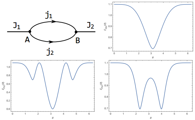
Figure 1. (color online) Sketch of the spin boundary state described by Eq.(6). The spins on dangling edges are taken as J1 = J2 = 1. The entanglement entropy as a function of θ with
${j}_{1}={j}_{2}=\frac{1}{2}$ (upper right); j1 = j2 = 1 (lower left); and j1 = 2, j2 = 1(lower right).where N is the normalization coefficient,
${C}_{M\,{m}_{1}\,{m}_{1}}^{J\,{j}_{1}\,{j}_{2}}=\langle {j}_{1}\,{m}_{1};{j}_{2}\,{m}_{2}|J\,M\rangle $ is the standard Clebsch-Gordan coefficient, and Dmn = (-1)j-mδm, -n is the virtual two-valent intertwiner denoting the direction of the holonomy.${U}_{{n}_{i}}^{{k}_{i}}$ is the matrix representation of the holonomy along the edge with ji. In particular, we specify the group elements for each holonomy as${U}_{{n}_{i}}^{{k}_{i}}(g(\theta ))={e}^{-i{k}_{i}\theta }{\delta }_{{n}_{i}}^{{k}_{i}}$ , where θ is the group parameter. For simplicity, we also ignore the holonomy along dangling edges, where they are uniformly taken as the unit element of SU(2).We now consider the entanglement entropy for this bipartite system. We choose A = {J1} and B = {J2}, so that the reduced density matrix is given by ρA = TrB(|ΨJ1; J2〉〈 ΨJ1; J2|). As a result, the entanglement entropy can be evaluated as
$ \begin{eqnarray}{E}_{{\rho }_{A}}(\theta )=-{\rm{Tr}}(\frac{{\rho }_{A}{\rm{ln}}{\rho }_{A}}{\langle {{\rm{\Psi }}}_{{J}_{1};{J}_{2}}|{{\rm{\Psi }}}_{{J}_{1};{J}_{2}}\rangle }).\end{eqnarray} $
(7) The numerical results for various spins are shown in Fig. 1. Firstly, we note that the entanglement entropy is not independent of the group elements any more; it is a function of the parameter θ. Secondly, we find that the entropy satisfies the bounds |ln(2j1 + 1)-ln(2j2 + 1)|≤EρA(θ)≤ln(2j1 + 1) + ln(2j2 + 1). In fact, in this special case, since there is only one dangling edge at each vertex, a stronger upper bound holds EρA(θ)≤min{ln(2J1 + 1), ln(2J2 + 1)}. It is also interesting to note that the entanglement entropy vanishes for θ = π (lower left plot of Fig. 1), which means that it is simply a direct product state.
Next, we consider the case that two vertices are linked by more than one path, which means that some paths may connect them indirectly by passing through other vertices. This is, of course, a common case for general spin networks. As an example, we consider the spin network shown in Fig. 2. The corresponding boundary state is given as
$ \begin{eqnarray}\begin{array}{ll}|{{\rm{\Psi }}}_{{J}_{1}{J}_{4};{J}_{2}{J}_{3}}\rangle&=\displaystyle \sum _{{M}_{l}}N{C}_{{M}_{1}{m}_{1}{k}_{4}}^{{J}_{1}{j}_{1}{j}_{4}}{D}^{{m}_{1}{n}_{1}}{U}_{{n}_{1}}^{{k}_{1}* }(g(\theta ))\\&\times {C}_{{M}_{2}{m}_{2}{k}_{1}}^{{J}_{1}{j}_{2}{j}_{1}}{D}^{{m}_{2}{n}_{2}}{U}_{{n}_{2}}^{{k}_{2}* }(g(0)){C}_{{M}_{3}{m}_{3}{k}_{2}}^{{J}_{3}{j}_{3}{j}_{2}}\\&\times {D}^{{m}_{3}{n}_{3}}{U}_{{n}_{3}}^{{k}_{3}* }(g(0)){C}_{{M}_{4}{m}_{4}{k}_{3}}^{{J}_{4}{j}_{4}{j}_{3}}{D}^{{m}_{4}{n}_{4}}\\&\times {U}_{{n}_{4}}^{{k}_{4}* }(g(0))|{M}_{1}{M}_{2}{M}_{3}{M}_{4}\rangle,\end{array}\end{eqnarray} $
(8) 
Figure 2. (color online) Sketch of the boundary state described by Eq.(8). The spins on dangling edges are taken as Ji = 1(i = 1,
$ \ldots $ 4). The entanglement entropy as a function of θ with${j}_{i}=\frac{1}{2}(i=1,\ldots 4)$ (upper right); ji = 1 (i = 1,$ \ldots $ 4) (lower left); and j1 = j3 = 2, j2 = j4 = 1 (lower right).where, for a bipartite system, we have chosen A = {J1, J4} and B = {J2, J3} and l = 1, … 4. The reduced density matrix for the bipartite entanglement entropy is given as ρA = TrB(|ΨJ1 J4; J2 J3〉〈 ΨJ1J4; J2 J3|). Numerical results for a few specific spins are shown in Fig. 2. We note that the entanglement entropy is generally a function of the parameter θ. In particular, when two parts are linked by two edges with spins j1 and j3, respectively, we find that the entropy is bounded as |ln(2j1 + 1)-ln(2j3+1) |≤EρA(θ)≤ln(2j1 + 1)+ln(2j3 + 1).
-
In this section, we take the intertwiner entanglement into account. In ref. [19], it was shown that when two neighboring vertices A and B are linked by a single edge carrying a spin j, as shown in Fig. 3(1), then the total entanglement entropy of the boundary states can be separated into two parts, one from intertwiner entanglement at vertices and the other from spin entanglement, which is nothing but ln(2j + 1), the maximal entropy allowed by the spin on the edge and independent of the group elements of the holonomy. We point out that the following relation plays a crucial role in the separation of spin entanglement and intertwiner entanglement; it is the orthogonal relation between two intertwiners
$ \;\;\;\;\displaystyle \sum _{{N}_{1}\cdots {N}_{q}}\langle {I}^{{k}_{2}}|{N}_{1}\cdots {N}_{q}m\rangle \langle {N}_{1}\cdots {N}_{q}{m}^{\prime}|{I}^{{{k}^{\prime}}_{2}}\rangle \\ =\frac{1}{2j+1}{\delta }_{{k}_{2}{{k}^{\prime}}_{2}}{\delta }_{m{m}^{\prime}}, $
(9) 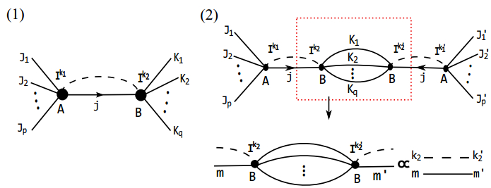
Figure 3. (color online) (1) Two neighboring vertices A and B are linked by a single edge carrying a spin j. The dashed line denotes the entanglement of two interwiners. (2) The sketch of the orthogonal relation described by Eq.(9).
where |Ik2〉 represents the k2-th component of the intertwiner state, and Ni (i = 1, …, q) is the magnetic quantum number of the spin on the i-th dangling edge, while m is the magnetic quantum number of the spin j on the single edge linking two vertices.
This orthogonal relation can be represented as a diagram, as shown in Fig. 3(2). Obviously, this identity is applied during the evaluation of the reduced density matrix such that the final result can be written as a product of the spin contribution and the intertwiner contribution, as shown in Eq. (24) in [19].
However, when two vertices are linked by two or more edges, we find that this situation does not hold any more. In general, the bipartite entanglement entropy can not be separated into a spin part and an intertwiner part. For explicitness, we consider two vertices A and B linked by two edges carrying spin j1 and j2, respectively, as shown in Fig. 4(1). For the evaluation of the reduced density matrix, we need to simplify the contractions of tensors. Unfortunately, we find that the following identity, needed to separate the intertwiner entanglement from spin entanglement, does not hold,
$ \;\;\;\;\displaystyle \sum _{{N}_{1}\cdots {N}_{q}}\langle {I}^{{k}_{2}}|{N}_{1}\cdots {N}_{q}{m}_{1}{m}_{2}\rangle \langle {N}_{1}\cdots {N}_{q}{{m}^{\prime}}_{1}{{m}^{\prime}}_{2}|{I}^{{{k}^{\prime}}_{2}}\rangle \\ \ne \frac{1}{(2{j}_{1}+1)(2{j}_{2}+1)}{\delta }_{{k}_{2}{{k}^{\prime}}_{2}}{\delta }_{{m}_{1}{{m}^{\prime}}_{1}}{\delta }_{{m}_{2}{{m}^{\prime}}_{2}}, $
(10) 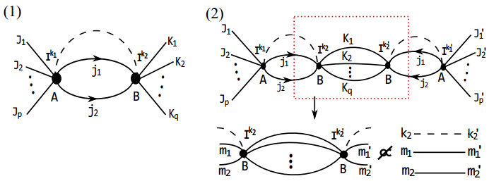
Figure 4. (color online) (1) Two neighboring vertices A and B are linked by two edges carrying spin j1 and j2, respectively. (2) The extension of the orthogonal relation does not hold.
This is diagrammatically sketched in Fig. 4(2). We provide the proof for this statement in the Appendix. Similarly, one can show that such relations are also absent when two vertices are linked by more than two edges indirectly. Therefore, for a general spin network with dangling edges, it is not possible to separate the total entropy into the contributions from spins on the edges and from intertwiners at vertices.
The above orthogonal relation is not a necessary condition for separating the intertwiner indices and spin indices. However, we remark that, in a general case, they can not be separated if two vertices are linked by more than one path. To support this statement, we evaluate the total entanglement entropy and the intertwiner entanglement entropy numerically for a few specific spin networks. An example is shown in Fig. 5, and the boundary spin state reads
$ \begin{eqnarray}\begin{array}{ll}|{\rm{\Psi }}\rangle&=\displaystyle \sum _{{M}_{i}{N}_{i}}\frac{{\varphi }_{{k}_{1}{k}_{2}}}{\sqrt{(2{k}_{1}+1)(2{k}_{2}+1)}}{C}_{{n}_{1}{M}_{1}{M}_{2}}^{{k}_{1}{J}_{1}{J}_{2}}{C}_{{{n}^{\prime}}_{1}{m}_{1}{m}_{2}}^{{k}_{1}{j}_{1}{j}_{2}}\\&\times {D}^{{n}_{1}{{n}^{\prime}}_{1}}{C}_{{{n}^{\prime}}_{2}{{m}^{\prime}}_{1}{{m}^{\prime}}_{2}}^{{k}_{2}{j}_{1}{j}_{2}}{C}_{{n}_{2}{N}_{1}{N}_{2}}^{{k}_{2}{K}_{1}{K}_{2}}{D}^{{n}_{2}{{n}^{\prime}}_{2}}{D}^{{m}_{1}{{m}^{\prime}}_{1}}\\&\times {D}^{{m}_{2}{{m}^{\prime}}_{2}}|{M}_{1}{M}_{2}{N}_{1}{N}_{2}\rangle,\end{array}\end{eqnarray} $
(11) 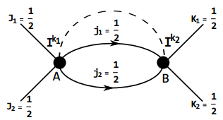
Figure 5. Sketch of the boundary spin state with intertwiner entanglement described by Eq. (11).
where i = 1, 2 and k1, k2 are possible spins on virtual edges inside intertwiner A and B, respectively.
If we take all spins on the dangling edges to be
$\frac{1}{2}$ , then the spins on virtual edges inside an intertwiner can be 0 and 1. With this assumption, the boundary state takes the following general form,$ \begin{eqnarray}\begin{array}{ll}|{\rm{\Psi }}\rangle&=\displaystyle \sum _{{M}_{i}{N}_{i}}({\varphi }_{00}{C}_{0{M}_{1}{M}_{2}}^{0\frac{1}{2}\frac{1}{2}}{C}_{0{N}_{1}{N}_{2}}^{0\frac{1}{2}\frac{1}{2}}\\&+\frac{1}{3}{\varphi }_{11}{C}_{{n}_{1}{M}_{1}{M}_{2}}^{1\frac{1}{2}\frac{1}{2}}{C}_{{n}_{2}{N}_{1}{N}_{2}}^{1\frac{1}{2}\frac{1}{2}}{D}^{{n}_{1}{n}_{2}})|{M}_{1}{M}_{2}{N}_{1}{N}_{2}\rangle,\end{array}\end{eqnarray} $
(12) where
$\varphi $ 00 and$\varphi $ 11 are two components in the intertwiner space. It should be noted that the other two components$\varphi $ 01 and$\varphi $ 10 do not appear in the above equation simply because the contraction of the corresponding CG coefficients in these terms vanishes.The reduced density matrix for bipartition is given as ρM1M2 = TrN1N2(|Ψ〉〈Ψ|). It is straightforward to obtain the entanglement entropy, which is
$ \begin{eqnarray}\begin{array}{lll}E&=&-{\rm{Tr}}(\frac{{\rho }_{{M}_{1}{M}_{2}}{\rm{ln}}{\rho }_{{M}_{1}{M}_{2}}}{\langle {\rm{\Psi }}|{\rm{\Psi }}\rangle })\\&=&-\frac{3{|{\varphi }_{00}|}^{2}}{3{|{\varphi }_{00}|}^{2}+{|{\varphi }_{11}|}^{2}}{\rm{ln}}({|{\varphi }_{00}|}^{2})\\&& -\frac{{|{\varphi }_{11}|}^{2}}{3{|{\varphi }_{00}|}^{2}+{|{\varphi }_{11}|}^{2}}{\rm{ln}}({|{\varphi }_{11}|}^{2})\\&& +\frac{{|{\varphi }_{11}|}^{2}-3{|{\varphi }_{00}|}^{2}}{3{|{\varphi }_{00}|}^{2}+{|{\varphi }_{11}|}^{2}}{\rm{ln}}3+{\rm{ln}}(3{|{\varphi }_{00}|}^{2}+{|{\varphi }_{11}|}^{2}).\end{array}\end{eqnarray} $
(13) On the other hand, the intertwiner entanglement entropy is determined by the matrix
$\varphi $ k1k2,$ \begin{eqnarray}{\varphi }_{{k}_{1}{k}_{2}}=\left(\begin{array}{cc}{\varphi }_{00}&{\varphi }_{01}\\ {\varphi }_{10}&{\varphi }_{11}\end{array}\right).\end{eqnarray} $
(14) The reduced density matrix is
${\rho }_{{k}_{1}}=\frac{{\varphi }_{{k}_{1}{k}_{2}}{\varphi }_{{k}_{1}{k}_{2}}^{\dagger }}{Tr({\varphi }_{{k}_{1}{k}_{2}}^{\dagger }{\varphi }_{{k}_{1}{k}_{2}})}$ . The entanglement entropy between intertwiners is$ \begin{eqnarray}{E}_{I}=-{\rm{Tr}}({\rho }_{{k}_{1}}{\rm{ln}}{\rho }_{{k}_{1}})=-({a}_{+}{\rm{ln}}{a}_{+}+{a}_{-}{\rm{ln}}{a}_{-}),\end{eqnarray} $
(15) where
$ \begin{eqnarray*}{a}_{\pm }=\left(\frac{1}{2}\pm \frac{1}{2}\sqrt{1-\frac{4{|{\varphi }_{00}{\varphi }_{11}-{\varphi }_{01}{\varphi }_{10}|}^{2}}{{|{\varphi }_{00}|}^{2}+{|{\varphi }_{01}|}^{2}+{|{\varphi }_{10}|}^{2}+{|{\varphi }_{11}|}^{2}}}\,\right).\end{eqnarray*} $
In Table 1, we evaluate the entanglement entropy E of the boundary spin state and the entanglement entropy EI of intertwiners for a few specific values of intertwiner parameters. It manifestly indicates that the total entanglement entropy measured in boundary states can not be written as the sum of the spin contribution and the intertwiner contribution. For instance, in the fifth column of the table, the entanglement entropy between intertwiners is even larger than the entanglement entropy for the boundary state. In the last column, the total entanglement entropy of the boundary state is zero, but the entanglement of intertwiners is not. In the next-to-last column, "meaningless" means that the boundary state |Ψ 〉 vanishes. Finally, we remark that the total entanglement entropy is not larger than ln4 in all cases considered, simply because all dangling edges carry spin 1/2. In general, the bounds we found in the previous section do not hold any more when the intertwiner entanglement is involved.
$\varphi $ k1k2$(\begin{array}{ll}1&0\\ 0&0\end{array})$ $(\begin{array}{ll}1&0\\ 0&1\end{array})$ $(\begin{array}{ll}1&0\\ 0&3\end{array})$ $(\begin{array}{ll}3&0\\ 0&1\end{array})$ $(\begin{array}{ll}1&1\\ 1&1\end{array})$ $(\begin{array}{ll}1&\sqrt{3}\\ \sqrt{3}&3\end{array})$ $(\begin{array}{ll}0&1\\ 1&0\end{array})$ $(\begin{array}{ll}1&1\\ 1&0\end{array})$ E 0 ${\rm{ln}}4-\frac{1}{2}{\rm{ln}}3$ ln 4 ${\rm{ln}}28-\frac{20}{7}{\rm{ln}}3$ ${\rm{ln}}4-\frac{1}{2}{\rm{ln}}3$ ln 4 meaningless 0 EI 0 ln2 ${\rm{ln}}10-\frac{9}{5}{\rm{ln}}3$ ${\rm{ln}}10-\frac{9}{5}{\rm{ln}}3$ 0 0 ln2 $-\frac{3+\sqrt{5}}{6}{\rm{ln}}(\frac{3+\sqrt{5}}{6})$ $-\frac{3-\sqrt{5}}{6}{\rm{ln}}(\frac{3-\sqrt{5}}{6})$ Table 1. The entanglement entropy E of boundary spin state and the entanglement entropy EI of intertwiners for various intertwiner matrices.
-
In this paper, we have investigated the bipartite entanglement for the boundary spin states in spin networks with dangling edges. In particular, we have constructed a simple type of spin network in which two complementary parts are linked by two paths, either in a direct or indirect manner. The numerical evaluation of entanglement entropy leads to the following two main results. Firstly, in the absence of the intertwiner entanglement, the entanglement entropy for the boundary state depends on the group elements of the holonomy, which can not be simply determined by the spins j1 and j2 on the edges connecting the complementary parts. Nevertheless, we have proposed a bound for the entanglement entropy, which is |ln(2j1 + 1)-ln(2j2 + 1)|≤E≤ln(2j1 + 1)+ln(2j2 + 1). It would be very important to prove or test this bound in a general case. Secondly, when the intertwiner entanglement is taken into account, the total entanglement can not be written, in general, as the sum of intertwiner entanglement and spin entanglement, but as a mixture of these two contributions.
Although we have only considered the simple case with two paths connecting two vertices, we believe that the above statements could be applicable to more complicated cases in which two vertices are linked by more than two edges directly, or by indirect paths.
Finally, based on our current work it is quite intriguing to further explore the relationship between quantum entanglement and quantum geometry, described by spin network states in loop quantum gravity. Our investigation is in progress and will be published in the near future [21].
We are very grateful to Yuxuan Liu and Zhuoyu Xian for helpful discussions and suggestions.
-
In this Appendix, we demonstrate the absence of the orthogonal relation for intertwiners when two vertices are linked by two edges, namely the inequality in Eq. (10), by applying the proof by contradiction. Assume that Eq. (10) is true. Let us consider the following contraction, which appears in the evaluation of the reduced density matrix
$ \begin{eqnarray}\begin{array}{ll}D=&\displaystyle \sum _{{N}_{1}\cdots {N}_{q}}\langle {I}^{{k}_{2}}|{N}_{1}\cdots {N}_{q}{m}_{1}{m}_{2}\rangle \displaystyle \sum _{{k}_{2}^{\prime}}\langle {N}_{1}\cdots {N}_{q}{m}_{1}^{\prime}{m}_{2}^{\prime}|{I}^{{k}_{2}^{\prime}}\rangle \\&\times \langle {I}^{{k}_{2}^{\prime}}|{M}_{1}\cdots {M}_{p}{m}_{1}^{^{\prime\prime} }{m}_{2}^{^{\prime\prime} }\rangle .\end{array}\end{eqnarray} $
(A1) From Eq.(10), one can write Eq.(A1) as,
$ \begin{eqnarray}D=\frac{1}{(2{j}_{1}+1)(2{j}_{2}+1)}{\delta }_{{m}_{1}{m}_{1}^{\prime}}{\delta }_{{m}_{2}{m}_{2}^{\prime}}\,\langle {I}^{{k}_{2}}|{M}_{1}\cdots {M}_{p}{m}_{1}^{^{\prime\prime} }{m}_{2}^{^{\prime\prime} }\rangle \end{eqnarray} $
(A2) For convenience, we define the operator
$\hat{P}=\displaystyle \sum |{I}^{{k}_{2}^{\prime}}\rangle \langle {I}^{{k}_{2}^{\prime}}|$ , so that Eq. (A1) can be rewritten as$ \begin{eqnarray}\begin{array}{ll}D=&\displaystyle \sum _{{N}_{1}\cdots {N}_{q}}\langle {I}^{{k}_{2}}|{N}_{1}\cdots {N}_{q}{m}_{1}{m}_{2}\rangle \\&\times \langle {N}_{1}\cdots {N}_{q}{m}_{1}^{\prime}{m}_{2}^{\prime}|\hat{P}|{M}_{1}\cdots {M}_{p}{m}_{1}^{^{\prime\prime} }{m}_{2}^{^{\prime\prime} }\rangle .\end{array}\end{eqnarray} $
(A3) A diagrammatic sketch of Eqs. (A1), (A2) and (A3) is shown in Fig. A1. We introduce the operator
${\hat{J}}^{2}={({\hat{J}}_{1}+{\hat{J}}_{2})}^{2}$ . The action of operators${\hat{J}}_{1}$ and${\hat{J}}_{2}$ is defined as$ \begin{eqnarray}\begin{array}{c}\langle {m}_{1}{m}_{2}|{\hat{J}}_{1}|{m}_{1}^{\prime}{m}_{2}^{\prime}\rangle =\langle {m}_{1}|{\hat{J}}_{1}|{m}_{1}^{\prime}\rangle {\delta }_{{m}_{2}{m}_{2}^{\prime}}\\ \langle {m}_{1}{m}_{2}|{\hat{J}}_{2}|{m}_{1}^{\prime}{m}_{2}^{\prime}\rangle ={\delta }_{{m}_{1}{m}_{1}^{\prime}}\langle {m}_{2}|{\hat{J}}_{2}|{m}_{2}^{\prime}\rangle,\end{array}\end{eqnarray} $
(A4) 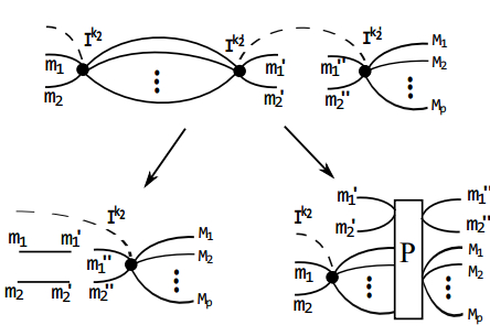
Figure A1. Diagrammatic sketch of the processes in Eqs. (A1), (A2), (A3).
where
${\hat{J}}_{i}^{2}|{j}_{i}m\rangle ={j}_{i}({j}_{i}+1)|{j}_{i}m\rangle $ (i = 1, 2). Next, we consider the following action of this operator on D, which is denoted as F and shown in Fig. A2.$ \begin{eqnarray}\begin{array}{ll}F=&\displaystyle \sum _{{N}_{1}\cdots {N}_{q}}\langle {I}^{{k}_{2}}|{N}_{1}\cdots {N}_{q}{m}_{1}{m}_{2}\rangle \displaystyle \sum _{{m}_{1}^{\prime}{m}_{2}^{\prime}}\langle {m}_{1}^{\prime\prime\prime }{m}_{2}^{\prime\prime\prime }|{\hat{J}}^{2}|{m}_{1}^{\prime}{m}_{2}^{\prime}\rangle \\&\times \langle {N}_{1}\cdots {N}_{q}{m}_{1}^{\prime}{m}_{2}^{\prime}|\hat{P}|{M}_{1}\cdots {M}_{p}{m}_{1}^{^{\prime\prime} }{m}_{2}^{^{\prime\prime} }\rangle .\end{array}\end{eqnarray} $
(A5) 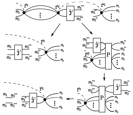
Figure A2. Diagrammatic sketch of the processes in Eqs. (A5), (A6), (A7), (A8), (A9).
On the one hand, by virtue of Eq. (A2), Eq. (A5) can be simplified as
$ \begin{eqnarray}\begin{array}{ll}F=&\frac{1}{(2{j}_{1}+1)(2{j}_{2}+1)}\langle {m}_{1}^{\prime\prime\prime }{m}_{2}^{\prime\prime\prime }|{\hat{J}}^{2}|{m}_{1}{m}_{2}\rangle \\&\times \langle {I}^{{k}_{2}}|{M}_{1}\cdots {M}_{p}{m}_{1}^{^{\prime\prime} }{m}_{2}^{^{\prime\prime} }\rangle .\end{array}\end{eqnarray} $
(A6) On the other hand, from Eq. (A3), we may rewrite Eq. (A5) as
$ \begin{eqnarray}\begin{array}{ll}F=&\displaystyle \sum _{{N}_{1}\cdots {N}_{q}}\langle {I}^{{k}_{2}}|{m}_{1}{m}_{2}{N}_{1}\cdots {N}_{q}\rangle \displaystyle \sum _{{m}_{1}^{\prime}{m}_{2}^{\prime}}\langle {m}_{1}^{\prime\prime\prime }{m}_{2}^{\prime\prime\prime }|{\hat{J}}^{2}|{m}_{1}^{\prime}{m}_{2}^{\prime}\rangle \\&\times \langle {N}_{1}\cdots {N}_{q}{m}_{1}^{\prime}{m}_{2}^{\prime}|\hat{P}|{M}_{1}\cdots {M}_{p}{m}_{1}^{^{\prime\prime} }{m}_{2}^{^{\prime\prime} }\rangle .\end{array}\end{eqnarray} $
(A7) Next, we prove that the operators
${\hat{J}}^{2}$ and$\hat{P}$ commute with each other. For any |Ψ 〉$ \in $ H1 ⊗ H2 ⊗ … Hp, we have$\hat{P}|{\rm{\Psi }}\rangle \in {{\rm{Inv}}}_{SU(2)}[{{\boldsymbol{H}}}_{1}\otimes {{\boldsymbol{H}}}_{2}\otimes \cdots {{\boldsymbol{H}}}_{p}]$ . We also know that$[{\hat{J}}^{2},{\hat{J}}_{1}+{\hat{J}}_{2}+\cdots {\hat{J}}_{p}]=0$ and$({\hat{J}}_{1}+{\hat{J}}_{2}+\cdots {\hat{J}}_{p})\hat{P}|{\rm{\Psi }}\rangle =0$ . So, we have$({\hat{J}}_{1}+{\hat{J}}_{2}+\cdots {\hat{J}}_{p}){\hat{J}}^{2}\hat{P}|{\rm{\Psi }}\rangle =0$ . That means${\hat{J}}^{2}\hat{P}|{\rm{\Psi }}\rangle \in {{\rm{Inv}}}_{SU(2)}[{{\boldsymbol{H}}}_{1}\otimes {{\boldsymbol{H}}}_{2}\otimes \cdots {{\boldsymbol{H}}}_{p}]$ . We conclude that$\hat{P}{\hat{J}}^{2}\hat{P}|{\rm{\Psi }}\rangle ={\hat{J}}^{2}\hat{P}|{\rm{\Psi }}\rangle $ . Because |Ψ〉 is arbitrary, we have$\hat{P}{\hat{J}}^{2}\hat{P}={\hat{J}}^{2}\hat{P}$ . If we take its transposed-conjugate$\hat{P}{\hat{J}}^{2}\hat{P}=\hat{P}{\hat{J}}^{2}$ , we get${\hat{J}}^{2}\hat{P}=\hat{P}{\hat{J}}^{2}$ , i.e.$[\hat{P},{\hat{J}}^{2}]=0$ . With this fact, Eq. (A7) becomes$ \begin{eqnarray}\begin{array}{ll}F=&\displaystyle \sum _{{N}_{1}\cdots {N}_{q}}\langle {I}^{{k}_{2}}|{N}_{1}\cdots {N}_{q}{m}_{1}{m}_{2}\rangle \\&\times \displaystyle \sum _{{m}_{1}^{\prime}{m}_{2}^{\prime}}\langle {N}_{1}\cdots {N}_{q}{m}_{1}^{\prime\prime\prime }{m}_{2}^{\prime\prime\prime }|\hat{P}|{M}_{1}\cdots {M}_{p}{m}_{1}^{\prime}{m}_{2}^{\prime}\rangle \\&\times \langle {m}_{1}^{\prime}{m}_{2}^{\prime}|{\hat{J}}^{2}|{m}_{1}^{^{\prime\prime} }{m}_{2}^{^{\prime\prime} }\rangle .\end{array}\end{eqnarray} $
(A8) With the help of Eq. (A2) and Eq. (A3), the above equation can be further simplified as
$ \begin{eqnarray}\begin{array}{ll}F=&\frac{1}{(2{j}_{1}+1)(2{j}_{2}+1)}{\delta }_{{m}_{1}{m}_{1}^{\prime\prime\prime }}{\delta }_{{m}_{2}{m}_{2}^{\prime\prime\prime }}\\&\times \displaystyle \sum _{{m}_{1}^{\prime}{m}_{2}^{\prime}}\langle {I}^{{k}_{2}}|{m}_{1}^{\prime}{m}_{2}^{\prime}{M}_{1}\cdots {M}_{p}\rangle \langle {m}_{1}^{\prime}{m}_{2}^{\prime}|{\hat{J}}^{2}|{m}_{1}^{^{\prime\prime} }{m}_{2}^{^{\prime\prime} }\rangle .\end{array}\end{eqnarray} $
(A9) A diagrammatic sketch of Eqs. (A5)-(A9) is shown in Fig. A2.
If we contract both Eq. (A6) and Eq. (A9) with 〈M1… Mp m″1m″2| Ik2〉, we get
$ \begin{eqnarray}\begin{array}{c}\langle {m}_{1}^{\prime\prime\prime }{m}_{2}^{\prime\prime\prime }|{\hat{J}}^{2}|{m}_{1}{m}_{2}\rangle \displaystyle \sum _{{k}_{2},{{m}^{^{\prime\prime} }}_{i},{M}_{l}}\langle {I}^{{k}_{2}}|{M}_{1}\cdots {M}_{p}{m}_{1}^{^{\prime\prime} }{m}_{2}^{^{\prime\prime} }\rangle \langle {M}_{1}\cdots {M}_{p}{m}_{1}^{^{\prime\prime} }{m}_{2}^{^{\prime\prime} }|{I}^{{k}_{2}}\rangle \\ ={\delta }_{{m}_{1}{m}_{1}^{\prime\prime\prime }}{\delta }_{{m}_{2}{m}_{2}^{\prime\prime\prime }}\displaystyle \sum _{{k}_{2},{{m}^{\prime}}_{i},{{m}^{^{\prime\prime} }}_{i},{M}_{l}}\langle {I}^{{k}_{2}}|{M}_{1}\cdots {M}_{p}{m}_{1}^{\prime}{m}_{2}^{\prime}\rangle \langle {m}_{1}^{\prime}{m}_{2}^{\prime}|{\hat{J}}^{2}|{m}_{1}^{^{\prime\prime} }{m}_{2}^{^{\prime\prime} }\rangle \langle {M}_{1}\cdots {M}_{p}{m}_{1}^{^{\prime\prime} }{m}_{2}^{^{\prime\prime} }|{I}^{{k}_{2}}\rangle,\end{array}\end{eqnarray} $
(A10) where i = 1, 2 and l = 1, … p. Although this equation looks complicated, as there exist k2, M1, … Mp, m″1, m″2, such that
$\langle {I}^{{k}_{2}}|{M}_{1}\cdots {M}_{p}{m}_{1}^{^{\prime\prime} }{m}_{2}^{^{\prime\prime} }\rangle 0\ne $ , Eq. (A10) is nothing else but$ \begin{eqnarray}\begin{array}{ll}\langle {m}_{1}^{\prime\prime\prime }{m}_{2}^{\prime\prime\prime }|{\hat{J}}^{2}|{m}_{1}{m}_{2}\rangle&=K{\delta }_{{m}_{1}{m}_{1}^{\prime\prime\prime }}{\delta }_{{m}_{2}{m}_{2}^{\prime\prime\prime }}\\&=K\langle {m}_{1}^{\prime\prime\prime }{m}_{2}^{\prime\prime\prime }|{m}_{1}{m}_{2}\rangle,\end{array}\end{eqnarray} $
(A11) where K
$ \in $ C is a constant. This means that${\hat{J}}^{2}$ has only one eigenvalue K. However, when${j}_{1}\ge \frac{1}{2}$ and${j}_{2}\ge \frac{1}{2}$ ,${\hat{J}}^{2}$ has at least two different eigenvalues (j1 + j2)(j1 + j2 + 1) and |j1-j2|(|j1 - j2| + 1). Therefore, our starting assumption is not true and the orthogonal relation as shown in Eq. (10) does not exist.


 DownLoad: