


 Abstract
 HTML
HTML Reference
 Related
 PDF
PDF


-
The Crab Nebula (
$ \sim $ 2 kpc from the Earth) is the remnant of a core-collapse supernova in 1054 AD, recorded in Chinese and Japanese chronicles [1]. Observations of the nebula have been carried out at every accessible wavelength, resulting in a remarkably well-determined spectral energy distribution (SED), making it a “standard candle” at several wavelengths up to very high energy (VHE). The Crab Nebula was the first VHE γ-ray source discovered by the Whipple Collaboration in 1989 [2]. To date, the VHE emission has been firmly detected by many ground-based experiments, including both air shower arrays [3-6] and imaging Cherenkov telescopes [7-9]. Although several GeV flares have been detected by AGILE and Fermi [10, 11], the γ-ray emission from the Crab Nebula is generally believed to be steady at higher energies. Recently, γ-rays with energy above 100 TeV have been detected from this source by HAWC [5] and Tibet AS$ \gamma $ [6]. The observed spectrum around 100 TeV is consistent with a smooth extrapolation of the lower-energy spectrum. As a reference VHE γ-ray source, the Crab Nebula is often used to check detector performance, including sensitivity, pointing accuracy, angular resolution, and so on.The non-thermal radiation of the Crab Nebula is characterized by an SED consisting of two components. The low-energy component extending from radio to γ-ray frequencies comes from synchrotron radiation by relativistic electrons. The high-energy component dominates the emission above
$ \sim $ 1 GeV and is produced via inverse Compton (IC) scattering of ambient seed photons by relativistic electrons [7]. The absence of a high-energy cutoff in the measured spectrum from the Crab Nebula up to about 400 TeV indicates that the primary electrons can reach at least sub-PeV energies [6].LHAASO (100.01
$ ^{\circ} $ E, 29.35$ ^{\circ} $ N) is a large hybrid extensive air shower (EAS) array being constructed at Haizi Mountain, 4410 m a.s.l., in Daocheng, Sichuan province, China [12]. It is composed of three sub-arrays: a 1.3 km$ ^2 $ array (KM2A) for γ-ray astronomy above 10 TeV and cosmic ray physics, a 78000 m$ ^2 $ water Cherenkov detector array (WCDA) for TeV γ-ray astronomy, and 18 wide field-of-view air Cherenkov/fluorescence telescopes (WFCTA) for cosmic ray physics from 10 TeV to 1 EeV. A considerable proportion of the LHAASO detectors have been operating since 2019 and the whole array will be completed in 2021. KM2A has a wide field-of-view (FOV) of$ \sim $ 2 sr and covers 60% of the sky within a diurnal observation. KM2A is unique for its unprecedented sensitivity at energies above 20 TeV. Even though only one half of KM2A has been operating for a few months, the sensitivity for γ-ray sources at energies above 50 TeV is already better than what has been achieved by previous observations.Here, we present the first observation of the “standard candle” Crab Nebula using the first 5 months of half-array LHAASO-KM2A data, from December 2019 to May 2020. Through this, the detector performance is thoroughly tested, including pointing accuracy, angular resolution, background rejection power, and flux determination.
-
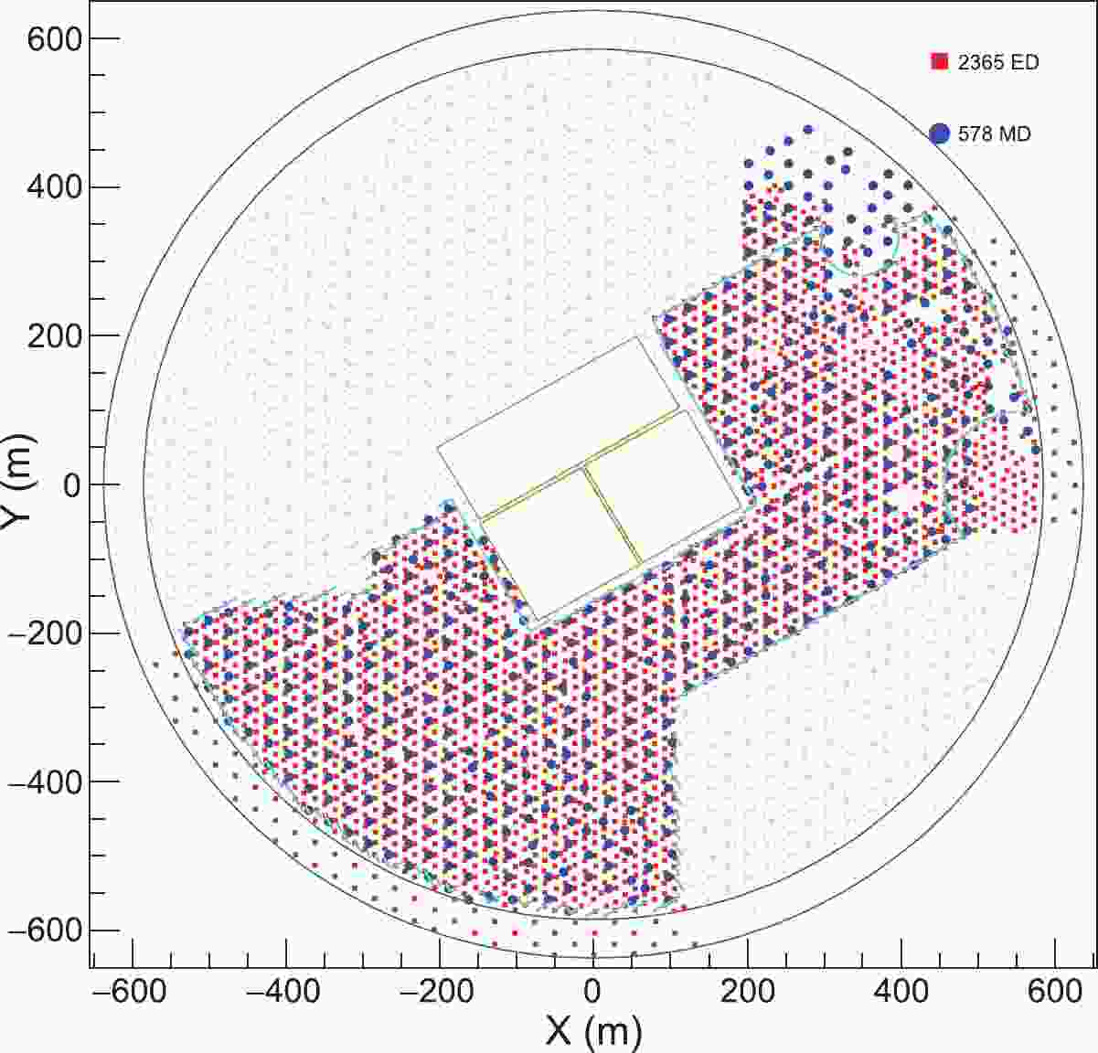
The whole KM2A array will consist of 5195 electromagnetic detectors (EDs, 1 m
$ ^2 $ each) and 1188 muon detectors (MDs, 36 m$ ^2 $ each), deployed over an area of 1.3 km$ ^2 $ as shown in Fig. 1. Within 575 m of the center of the array, EDs are distributed with a spacing of 15 m and MDs are distributed with a spacing of 30 m. Within the outskirt ring region of width 60 m, the spacing of EDs is enlarged to 30 m and these EDs are used to veto showers with cores located outside the central 1 km$ ^2 $ . KM2A operates around the clock, since both EDs and MDs can work during both day and night.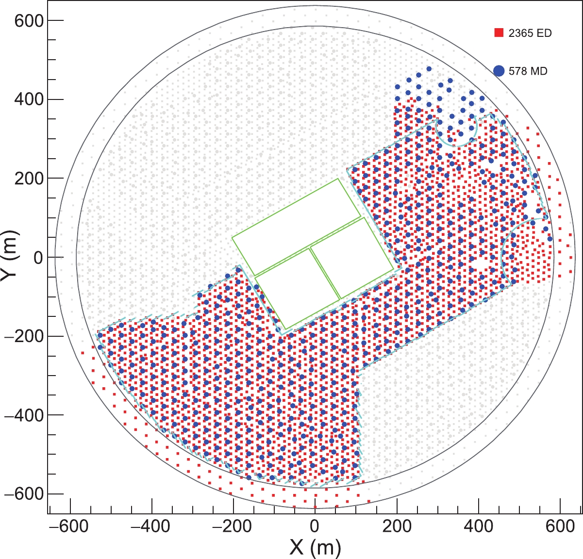
Figure 1. (color online) Planned layout of all LHAASO-KM2A detectors. The red squares and blue circles indicate the EDs and MDs in operation, respectively. The area enclosed by the cyan line outlines the fiducial area of the current KM2A half-array used in this analysis. The central green squares indicate the LHAASO-WCDA array region.
An ED consists of 4 plastic scintillation tiles (100 cm
$ \times $ 25 cm$ \times $ 1 cm each). More details about the ED design can be found elsewhere [12]. The coated tile is covered by a 5-mm-thick lead plate to absorb low-energy charged particles in showers and convert$ \gamma $ -rays into electron-positron pairs, which can improve the angular and core position resolution of the array. Once high energy charged particles enter the scintillator, they lose energy and excite the scintillation medium to produce a large number of scintillation photons. The embedded wavelength-shifting fibers collect scintillation light and transmit it to a 1.5-inch photomultiplier tube (PMT). The PMT records the arrival time and number of the particles, based on which the shower parameters can be reconstructed. The detection efficiency of a typical ED for minimum ionization particles is about 98%. The time resolution of an ED is about 2 ns. The charge resolution of the particle counter is$ < $ 25% for a single particle and the dynamic range is from 1 to 10$ ^4 $ particles. The average single rate of an ED is about 1.7 kHz with a threshold equivalent to 1/3 particle at the LHAASO site.The MD is a pure water Cherenkov detector enclosed within a cylindrical concrete tank with an inner diameter of 6.8 m and height of 1.2 m. An 8-inch PMT is installed at the center of the top of the tank to collect the Cherenkov light produced by high energy particles as they pass through the water. More details about the MD design can be found elsewhere [12]. The whole detector is covered by a steel lid underneath soil. The thickness of the overburden soil is 2.5 m, to absorb the secondary electrons/positrons and γ-ray in showers. Thus the particles that can reach the water inside and produce Cherenkov signals are almost exclusively muons, except for those MDs located at the very central part of showers where some very high energy EM components may have a chance to punch through the screening soil layer. The detection efficiency of a typical MD to muons is
$ > $ 95%. The time resolution of an MD is about 10 ns. The charge resolution of the particle counter is$ < $ 25% for a single muon and the dynamic range is from 1 to 10$ ^4 $ particles. The average single rate of an MD is about 8 kHz with a threshold equivalent to 0.4 particles at the LHAASO site.The KM2A detectors were constructed and merged into the data acquisition system (DAQ) in stages. The first 33 EDs started operating in February 2018 and the partial array was then enlarged step by step. Nearly half of the KM2A array, including 2365 EDs and 578 MDs and covering an area of 432000 m
$ ^2 $ as shown in Fig. 1, has been operating since 27 December 2019. The trigger logic of KM2A has been well tested and more details about it can be found elsewhere [13]. For the first half-array, at least 20 EDs firing within a window of 400 ns is required for a shower trigger, thus yielding a negligible random noise trigger rate. The event trigger rate is about 1 kHz. For each event, the DAQ records 10 μs of data from all EDs and MDs that have signals over the thresholds.The signal arrival time is measured by a time-to-digital converter (TDC) with a time precision of 1 ns and 2 ns for the EDs and MDs, respectively. The clock of each TDC node is synchronized via the so-called White Rabbit (WR) timing system with an accuracy of
$ \pm $ 150 ps. To further calibrate the detector response time, an offline method using the time residuals with respect to a reconstructed shower front plane is applied. More details about this method can be found elsewhere [14]. Figure 2 shows the calibrated timing offset for the EDs and MDs. The average delay in the response of the MDs relative to that of EDs is 119 ns. The standard deviations are 0.82 ns for the EDs and 6.7 ns for the MDs, which can be taken to represent the timing uncertainty of individual detectors. The timing calibration parameters are very stable and only need to be updated about every one or two months.
Figure 2. Distribution of calibrated timing offset for the EDs and MDs using experimental data on 1st May 2020. The average delay in the response of the MDs relative to that of EDs is 119 ns..
The signal charge is measured by an analog-to-digital converter (ADC). Based on the measurement of showers, the typical charge produced by a particle for each ED and MD was calibrated. With the charge calibration for each detector, the measured ADC counts were converted into the number of particles [14]. The calibration parameters for the EDs and MDS both vary with time because the system is affected by the temperature of the surroundings. The charge calibration parameters need to be updated every day. A variation of about 5% within each day remains uncorrected.
-
To estimate the properties of primary particles above the atmosphere, such as energy, composition, flux, etc, the simulation of the detector response is crucial. In this work, the cascade processes within the atmosphere were simulated via the CORSIKA code (version7.6400) [15]. To accurately simulate the KM2A detector response, a specific software, G4KM2A [16, 17], was developed in the framework of the Geant4 package (v4.10.00) [18]. De-correlated single rate noise and corresponding charges determined by the experimental data are also taken into account in this simulation. This software adopts a flexible strategy and can simulate the KM2A array with any configuration. The reliability of the detector simulation was verified via the partial KM2A array data [17]. Figure 3 shows the distribution of particle numbers recorded by a typical ED and MD. The simulation results are fairly consistent with experimental data. The change of the slope of the muon rate at N
$ _{\mu}> $ 10 is caused by the contamination of punch-through high energy electromagnetic particles in the core region of the shower.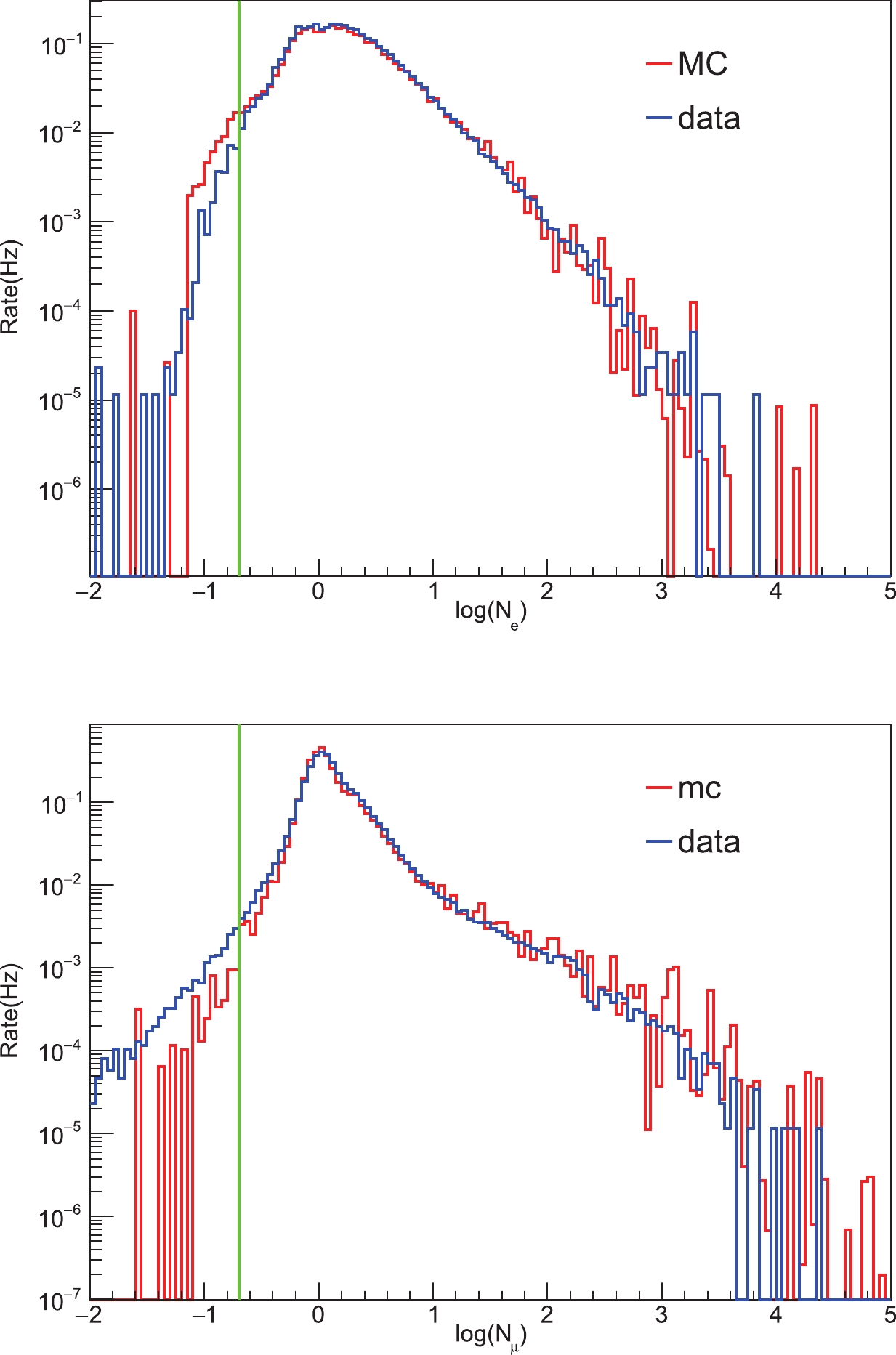
Figure 3. (color online) Comparison between MC simulation and experimental data of the daily averaged trigger rate distribution of a typical ED (upper panel) and MD (lower panel). The horizontal axes indicate the number of particles recorded by these detectors for the triggered events. Detectors with a particle number less than 0.2, as indicated by the vertical lines, are removed in both MC and experimental data reconstruction. The MC simulation, with five components, is normalized to the cosmic ray model of Ref. [19].
In this work, a data sample with 2.222
$ \times $ 10$ ^8 $ γ-ray shower and 4.444$ \times $ 10$ ^8 $ proton shower events was simulated. Both the γ-ray and proton events were sampled in the energy range from 1 TeV to 10 PeV following a power-law function with a spectral index of -2.0. The zenith angle is distributed from 0$ ^{\circ} $ to 70$ ^{\circ} $ . The sample area is a circular region with a sufficiently large radius of 1000 m.For a specific astrophysical source, the response of KM2A depends both on the source emission spectrum and the zenith angle within the detector FOV. With the above data sample, we need to re-weight the distribution of the zenith angle for γ-rays to trace the trajectory of the astrophysical source. In this work, the simulation data sample has been re-weighted to the sky trajectory of the Crab Nebula. In general the same data sample can be re-weighted for any astrophysical source of interest within the KM2A FOV. The response of KM2A for a different emission spectrum can also be simulated via further re-weighting on the primary spectrum. For the simulation data sample, the same reconstruction and analysis algorithms as for experimental data are adopted to extract the relevant quantities.
-
Each shower event is composed of many ED and MD hits, each of which has timing and charge information. In combination with the positions of these detectors, the primary direction and core location of the shower event can be reconstructed. For KM2A events, only the ED hits are used for direction, core location, and energy reconstruction. Both ED hits and MD hits are used for composition discrimination. For the experimental data selection, first the status of each detector is evaluated and abnormal EDs and MDs are removed. Then, each hit is calibrated for its timing and charge information to unify the detector response. Finally, both experimental and simulation events are processed through the same reconstruction pipeline.
For the event reconstruction, firstly, a time window of 400 ns and a circular window with a radius of 100 m are adopted to select the most probable real secondary shower hits. With these selected hits, the core location is reconstructed using an optimized centroid method and the direction is reconstructed by fitting the shower plane. Secondly, only hits within [−30, 50] ns perpendicular to the shower plane and with a distance less than 200 m from the shower core are selected. Using these hits, the core location, number of particles (i.e., shower size, denoted as N
$ _{\rm{size}} $ ) and shower age (denoted as s) are reconstructed using a likelihood method. The direction is also updated. Finally, all the ED and MD hits within [-30, 50] ns perpendicular to the reconstructed shower plane are selected. The final surviving ED hits are used to count the number of electromagnetic particles (denoted as N$ _{\rm{e}} $ ). To reduce pollution from the punch-through high energy electromagnetic particles near the shower core, only MDs further than 15 m from the core are used to obtain the number of muons N$ _{\mu} $ . The parameters N$ _{\mu} $ and N$ _{\rm{e}} $ are used to discriminate between γ-ray showers and cosmic ray showers.We show in Fig. 4 the pattern of a high energy γ-ray like shower (N
$ _{\mu} $ = 0) detected by KM2A from the Crab Nebula direction. Although there are many random noise hits during the recorded shower, the core location is evident from the distribution of particle density. The particle density and arrival time of the shower become clear after filtering out the noise hits via reconstruction.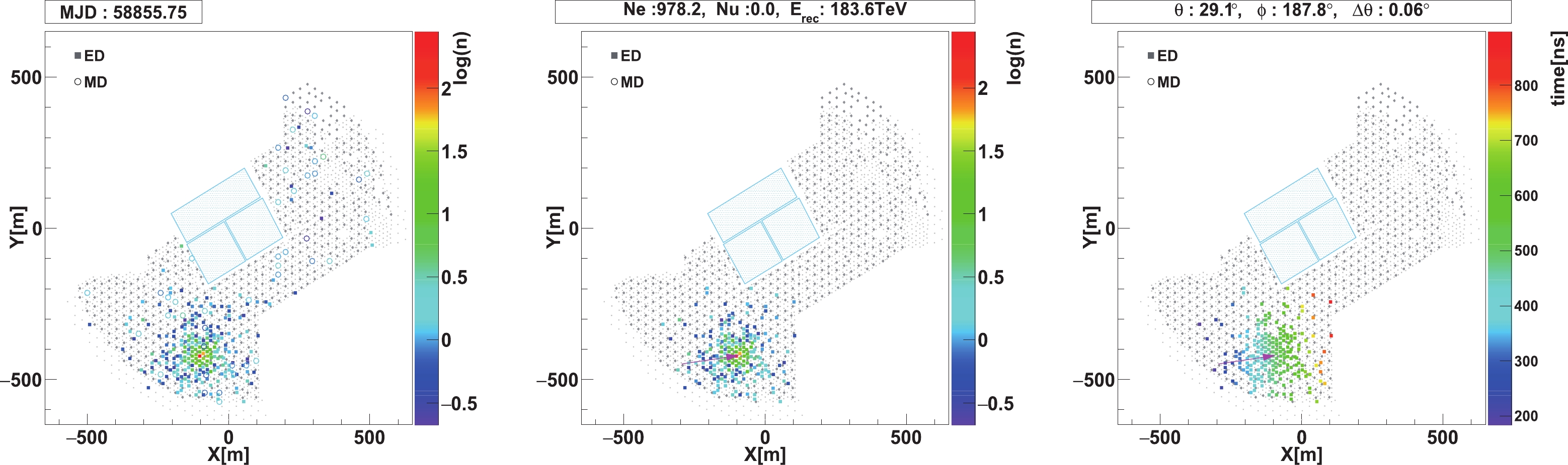
Figure 4. (color online) A high-energy γ-ray-like shower detected by KM2A from the Crab Nebula. Left: the original particle number of detector units in KM2A. Middle: the particle number map after filtering out noise hits that are clearly irrelevant to the reconstructed shower front. The number of fired EDs after filtering out the noise hits for this event is 202. The color scale indicates the logarithm of the particle number. Right: the unit map of the arrival time. The color scale indicates the relative trigger time of the unit in
${\rm ns}$ . E$_{\rm rec}$ denotes the reconstructed energy of the event.$\theta$ and$\phi$ denote the zenith angle and azimuth angle of the event, respectively. The magenta arrows shows the incident direction of the event.$\Delta\theta$ denotes the space angle between this event and the Crab Nebula direction.Before giving details about the core location, direction, energy reconstruction, effective area, and γ-ray/background discrimination, we list several data quality cuts: (1) the shower core is located in the fiducial area enclosed by the cyan lines in Fig. 1; (2) the zenith angle is less than 50
$ ^{\circ} $ ; (3) the number of particles detected within 40 m from shower core is larger than that within 40$ - $ 100 m; (4) the number of EDs and the number of particles for the reconstruction are both greater than 10; (5) the shower age is between 0.6 and 2.4. -
In an air shower, most of the secondary particles are distributed along the trajectory of the original primary particle. The expected position of the primary particle on the ground is defined as the shower core. Determining the core location is crucial for direction reconstruction, which will use the core location as a fixed vertex when fitting the shower front to a conical shape. The simplest method to reconstruct the core position consists of calculating the average of the fired detector coordinates weighted with the number of particles (denoted as
$ n_{\rm{e}} $ ). This simple algorithm is called the centroid method. It is fast in computing time, but turns out to be inadequate to perform a good core reconstruction. More refined techniques are needed. In this work, an optimized centroid method is implemented first. The functions are:$ {{\rm Core}x = }\frac{{\sum {{{{w}}_{{i}}}} {{{x}}_{{i}}}}}{{\sum {{{{w}}_{{i}}}} }},\;\;\;\;{{{\rm Core}y = }}\frac{{\sum {{{{w}}_{{i}}}} {{{y}}_{{i}}}}}{{\sum {{{{w}}_{{i}}}} }},\;\;\;\;{{{\rm Core}z = }}\frac{{\sum {{{{w}}_{{i}}}} {{{z}}_{{i}}}}}{{\sum {{{{w}}_{{i}}}} }}, $

(1) where
$ {{{w}}_{{i}}}$ =${{{n}}_{\rm{e}}}{{\rm{e}}^{{\rm{ - 0}}.{\rm{5}}{{({{{r}}_{{i}}}{\rm{/15}})}^{\rm{2}}}}}$ , (x$ _{{i}} $ , y$ _{{i}} $ , z$ _{{i}} $ ) are the ED coordinates,$ r_{{i}} $ is the ED distance to the shower core, and the units are m. The calculation needs about 20 iterations before converging. The obtained core location is used to filter out noise hits and as an initial value for further core reconstruction.The core is further reconstructed by fitting the lateral distribution function of the shower. The lateral distribution of particle density measured by the KM2A array is fitted using the following modified Nishimura-Kamata-Greisen (NKG) function [20]:
$ \rho ({{r}}){\rm{ = }}\frac{{{{{N}}_{{\rm{size}}}}}}{{{\rm{2}}\pi {{r}}_{\rm{m}}^{\rm{2}}}}\frac{{\Gamma ({\rm{4}}.{{5 - s}})}}{{\Gamma ({{s - 0}}.{\rm{5}})\Gamma ({{5 - 2s}})}}{\left(\frac{{{r}}}{{{{{r}}_{\rm{m}}}}}\right)^{{{s - 2}}.{\rm{5}}}}{\left({\rm{1 + }}\frac{{{r}}}{{{{{r}}_{\rm{m}}}}}\right)^{{{s - 4}}.{\rm{5}}}},$

(2) where r is the distance to the air shower axis, N
$ _{\rm{size}} $ is the total number of particles, s is the age of the shower, and r$ _{\rm{m}} $ is the Molière radius. r$ _{\rm{m}} $ is fixed at 136 m, following Ref. [21]. The reconstructed parameters are the core location, N$ _{\rm{size}} $ and s. The MINUIT package [22] is used to maximize the log likelihood by varying the parameters via two steps. Firstly, the core location is reconstructed with s = 1.2. Secondly, N$ _{\rm{size}} $ and s are reconstructed with the core location fixed at values obtained from the first step. Figure 5 shows the lateral distribution and corresponding fitting result of the γ-ray-like event shown in Fig. 4.
Figure 5. (color online) The solid curve shows the modified NKG function (2) that fits the data. The energy is 184
$\pm$ 31 TeV.The core resolution is energy and zenith dependent. The core resolution for γ-ray events over various zenith angle ranges is shown in Fig. 6 as a function of the reconstructed energy. The resolution (denoted as R
$ _{68} $ , containing 68% of the events) is about 4$ - $ 9 m at 20 TeV and 2$ - $ 4 m at 100 TeV.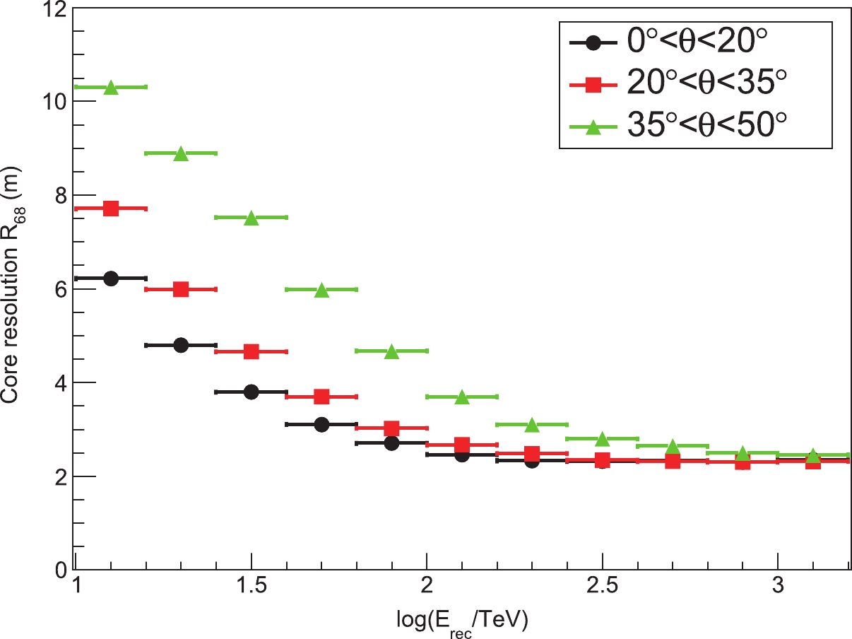
Figure 6. (color online) Core resolution of the KM2A half-array for simulated γ-ray showers over different zenith angle ranges.
-
The secondary particles of a shower travel roughly in a plane perpendicular to the direction of the primary particle, at the speed of light, as illustrated in Fig. 4. The direction can be reconstructed by fitting the shower plane. In fact, the shower front has a slightly conical shape, which needs to be accounted for when performing a good direction reconstruction. The arrival times of the particles are fitted by minimizing the following quantity:
$ {\chi ^{\rm{2}}}{\rm{ = }}\frac{{\rm{1}}}{{{{{N}}_{{\rm{hit}}}}}}\sum\limits_{{{i = 1}}}^{{{i = }}{{{N}}_{{\rm{hit}}}}} {{{{w}}_{{i}}}} \left({{{t}}_{{i}}}{\rm{ - l}}\frac{{{{{x}}_{{i}}}}}{{{c}}}{{ - m}}\frac{{{{{y}}_{{i}}}}}{{{c}}}{{ - n}}\frac{{{{{z}}_{{i}}}}}{{{c}}}{\rm{ - }}\alpha \frac{{{{{r}}_{{i}}}}}{{{c}}}{\rm{ - }}{{{t}}_{\rm{0}}}\right),$

(3) where l = sin
$ \theta $ cos$ \phi $ , m = sin$ \theta $ sin$ \phi $ , n = cos$ \theta $ ,$ \theta $ and$ \phi $ are the direction angles,$ \alpha $ is the conical correction coefficient, and c = 0.2998 m/ns is the speed of light. The sum is over the triggered EDs, t$ _{{i}} $ is the measured time of the ith ED, x$ _{{i}} $ , y$ _{{i}} $ , z$ _{{i}} $ are the ED coordinates, r$ _{{i}} $ is the ED distance from the core in the shower plane, and w$ _{{i}} $ is a weight set according to the time residual and distance to the shower core, i.e., w =$ \zeta (\delta {{t}}) \cdot \xi ({{r}})$ . It is known that the distribution of time residuals relative to the shower front is asymmetric. Multiple scattering can lead to a broader arrival time distribution for delayed particles. To optimize the fit, a specific asymmetric weight method is adopted in this work to reduce the effect of the delayed particles. The weight is set according to:$ \begin{aligned}[b] &\zeta (\delta {{t}}){\rm{ = }}\left\{ {\begin{array}{*{20}{l}} {{{\rm 1}},\qquad \qquad \qquad ({\rm{ - 20}}\;{\rm{ns}} < \delta {{t}} < {\rm{0}}\;{\rm{ns}})}\\ {{{\rm{e}}^{{\rm{ - }}\frac{{\rm{1}}}{{\rm{2}}}{{(\frac{{\delta {{t}}}}{{{\rm{10}}}})}^{\rm{2}}}}},\qquad\; (\delta {{t}} > {\rm{0}}\;{\rm{ns}},\;\;\delta {{t}} < {\rm{ - 20}}\;{\rm{ns}})} \end{array}} \right.\\& \delta {{t = }}{{{t}}_{{i}}}{{ - l}}\frac{{{{{x}}_{{i}}}}}{{{c}}}{{ - m}}\frac{{{{{y}}_{{i}}}}}{{{c}}}{{ - n}}\frac{{{{{z}}_{{i}}}}}{{{c}}}{\rm{ - }}\alpha \frac{{{{{r}}_{{i}}}}}{{{c}}}{\rm{ - }}{{{t}}_{\rm{0}}},\qquad \qquad \end{aligned} $

(4) where the times are given in ns.
It is also known that the error in the arrival time increases with the distance from the shower core. An empirical function in Ref. [23] is used in this work to calculate the weight according to the distance from the shower core. The weight is
$ \xi ({{r}}){\rm{ = }}\frac{{\rm{1}}}{{\sqrt {{\rm{1 + }}{{\left({\rm{1}}.{\rm{6}}{{\left(\dfrac{{{r}}}{{{\rm{30}}}}{\rm{ + 1}}\right)}^{{\rm{1}}.{\rm{5}}}}\right)}^{\rm{2}}}} }},$

(5) where r is given in m.
The reconstructed parameters are the direction cosines l, m,
$ \alpha $ and the offset time t$ _{0} $ . n can be determined using the parameters l and m during iteration. The zenith angle$ \theta $ and azimuth angle$ \phi $ of the shower can be derived from the parameters l and m. The angular resolution is energy and zenith angle dependent. The angular resolution for γ-ray events is shown in Fig. 7 as a function of the reconstructed energy over different zenith angle ranges. The resolution (denoted as$ \phi $ $ _{68} $ , containing 68% of the events) is 0.5$ ^{\circ}- $ 0.8$ ^{\circ} $ at 20 TeV and 0.24$ ^{\circ}- $ 0.3$ ^{\circ} $ at 100 TeV.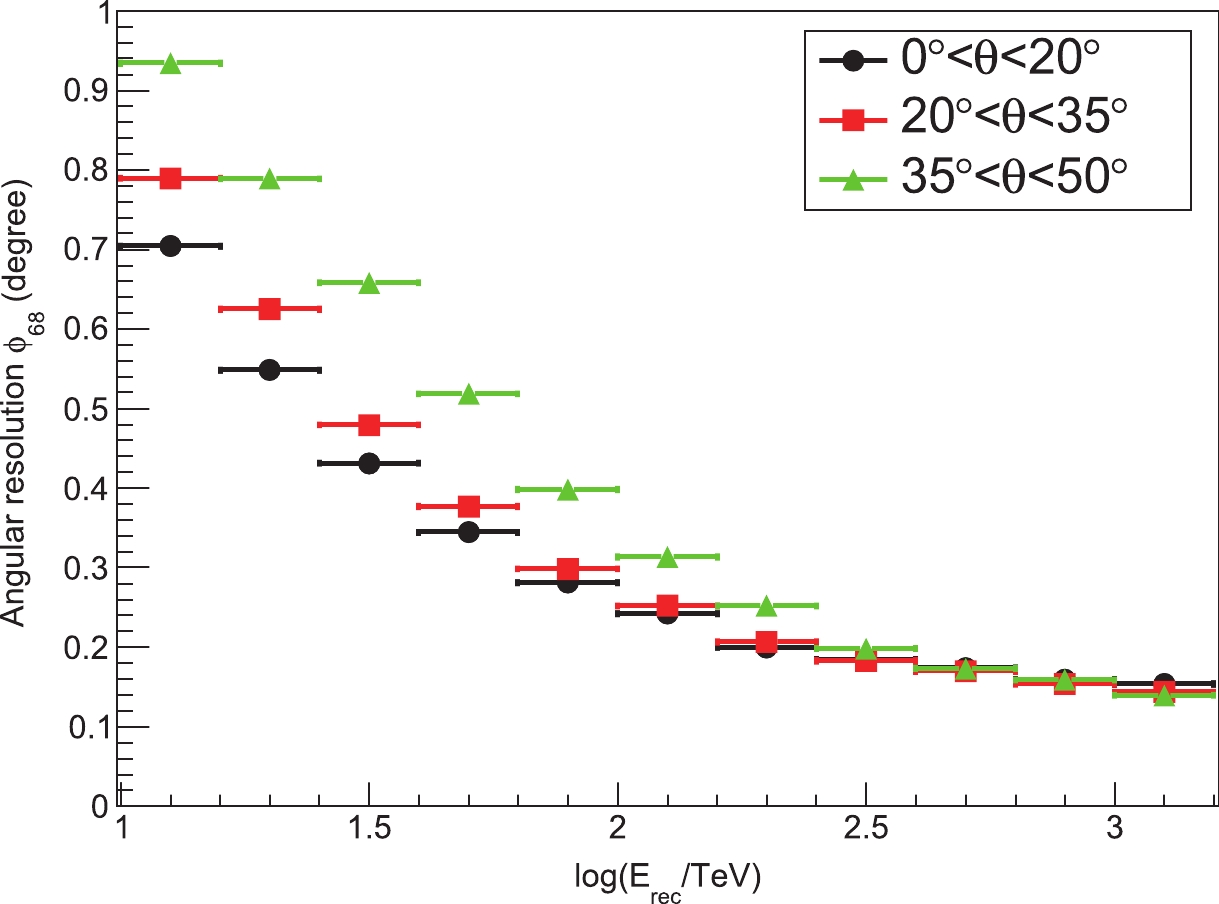
Figure 7. (color online) Angular resolution of the KM2A half-array for simulated γ-ray showers over different zenith angle ranges.
-
EAS arrays work by detecting the shower particles that reach ground level. A simple way to estimate a shower energy is to count the number of triggered detector elements, as used by the ARGO-YBJ experiment [24]. A robust estimator of a shower energy is to utilize the normalization of the lateral distribution function (LDF) of the shower as proposed by Ref. [25]. Usually, this is implemented by using the particle density at the optimal radius at which the uncertainty is minimized. This method has been used by Tibet AS
$ \gamma $ [26] and HAWC [5].The particle density at r = 50 m (denoted as
$ \rho_{50} $ ) evaluated using Eq. (2) is used to estimate the γ-ray energy in this work. The energy resolution values using densities from$ \rho_{40} $ to$ \rho_{70} $ are almost the same. Because the atmospheric depth over which the shower develops is proportional to sec($ \theta $ ), the zenith angle effect has to be taken into account in the energy reconstruction. The final response function between$ \rho_{50} $ and the primary energy is given by:$ {\rm{log}}({{{E}}_{{\rm{rec}}}}{\rm{/TeV}}){{ = a}}(\theta ) \cdot {({\rm{log}}({\rho _{{\rm{50}}}}))^{\rm{2}}}{{ + b}}(\theta ) \cdot {\rm{log}}({\rho _{{\rm{50}}}}){{ + c}}(\theta ), $

(6) where a
$ (\theta) $ , b$ (\theta) $ and c$ (\theta) $ are known constants, which have been given as functions of sec($ \theta $ ). The shower illustrated in Fig. 4 is estimated to have energy 184$ \pm $ 31 TeV using Eq. (6).The energy resolution is energy and zenith angle dependent. Figure 8 shows the relation between the reconstructed energy (E
$ _{\rm{rec}} $ ) and the primary true energy (E$ _{\rm{true}} $ ) over zenith angles 0$ ^{\circ} $ -50$ ^{\circ} $ . As the energy of the primary γ-ray increases, the shower maximum becomes closer to the altitude of the observatory, leading to better energy resolution. As the zenith angle increases, the shower maximum becomes higher, leading to a worse energy resolution. A slight asymmetry is visible in the reconstructed energy compared to the true energy. This is caused by the underestimation of energy for a fraction of showers, due to large fluctuations during the cascade process or large core reconstruction error. In this work, events with reconstructed energy above 10 TeV are divided into five bins per decade. The energy resolution for each energy bin over different zenith angles is shown in Fig. 8. For showers with zenith angle less than 20$ ^{\circ} $ , the resolution is about 24% at 20 TeV and 13% at 100 TeV.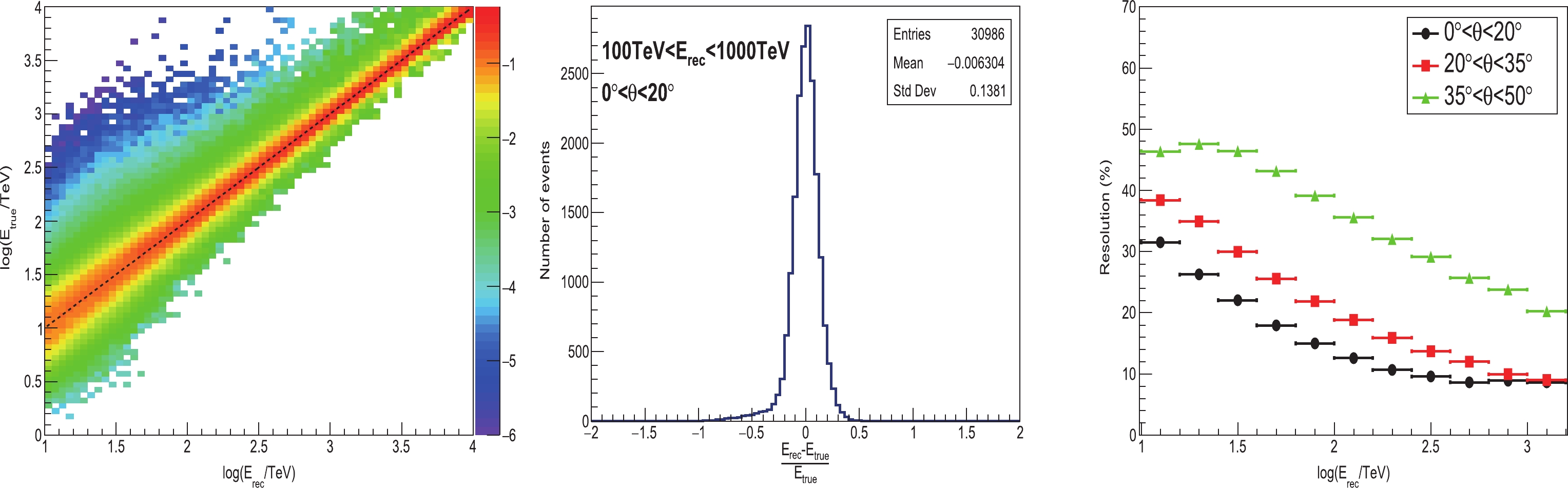
Figure 8. (color online) Left: event-by-event comparison of the primary true energy and the reconstructed energy for simulated γ-ray events over zenith angles 0
$^{\circ}$ -50$^{\circ}$ . The color represents the log probability density within each E$_{\rm{rec}}$ bin. The dotted line is the identity line. Middle: energy resolution function of showers in the energy range 100$-$ 1000 TeV with zenith angle 0$^{\circ}$ -20$^{\circ}$ . Right: dependence of energy resolution, defined as the half 68% width of the resolution function, on each reconstructed energy bin. The three colors indicate the resolutions over different zenith angle ranges. -
Most of the events recorded by KM2A are cosmic ray induced showers, which constitute the chief background for γ-ray observations. Considering that γ-ray induced showers are muon-poor and cosmic ray induced showers are muon-rich, the ratio between the measured muons and electrons is used to discriminate primary γ-rays from cosmic nuclei. The ratio is defined as:
$ {{R = {\rm log}}}\left(\frac{{{{{N}}_\mu }{\rm{ + 0}}.{\rm{0001}}}}{{{{{N}}_{\rm{e}}}}}\right), $

(7) where N
$ _{\mu} $ and N$ _{\rm{e}} $ are defined at the start of Sec. III, and 0.0001 is used to show the cases with N$ _{\mu} $ = 0. Figure 9 shows the ratio as a function of the reconstructed energy for γ-rays and protons. According to Fig. 9, the distributions of R for γ-rays and protons partly overlap at low energies due to wide N$ _{\mu} $ and N$ _{\rm{e}} $ fluctuations. The separation between γ-rays and protons becomes clearer at higher energies. For proton showers, the number of electrons detected by EDs is about 10 times the number of muons detected by MDs. This factor is about 1000 for γ-ray showers. The shower illustrated in Fig. 4 is a γ-ray-like event with N$ _{\mu} $ = 0.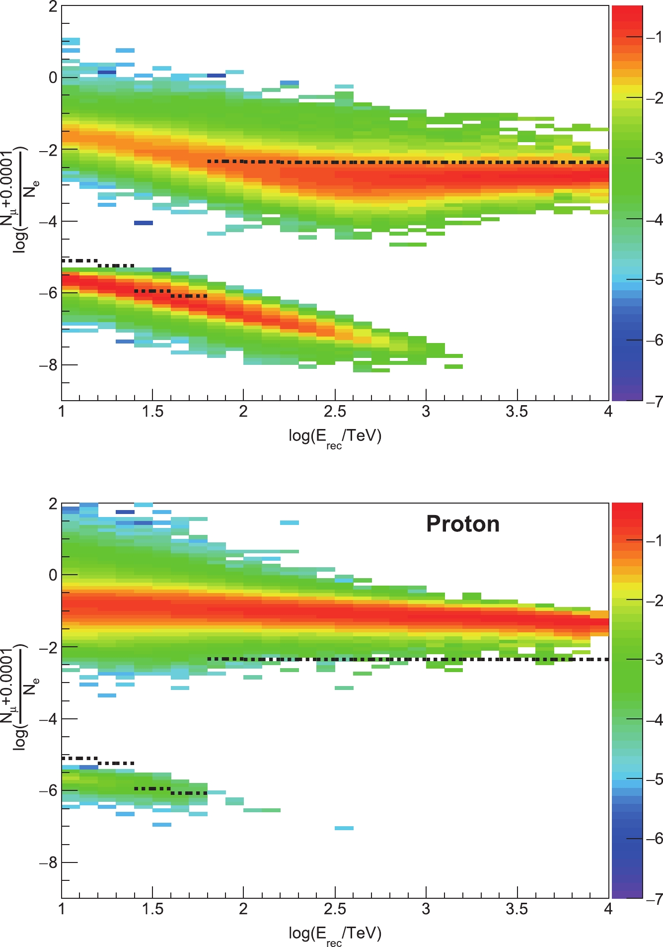
Figure 9. (color online) Scatter plot of R as defined in Eq. (7) vs. reconstructed energy using simulated γ-ray-induced (upper panel) and proton-induced (lower panel) air showers, respectively. The color represents the log probability density within each E
$_{\rm rec}$ bin. The dotted lines indicate the γ-ray/background discrimination cuts used in this work.γ-ray-like events are selected using simple cuts on the parameter R. These cuts depend on energy and are optimized to maximize the detection significance (defined by the Li-Ma formula, Eq. (17) of Ref. [27]) for a typical Crab-like source. This optimization consists of a mixture of γ-ray simulation and real off-source data recorded by KM2A, which are taken to represent the cosmic ray background. These cuts are shown in Fig. 9. Figure 10 shows the survival fraction for γ-ray showers (from simulation) along with the measured survival fraction for the cosmic ray background (from observational data) under these cuts. The fraction for γ-ray showers varies from 48% to 93%. The rejection power of cosmic ray induced showers is better than 4
$ \times $ 10$ ^{3} $ at energies above 100 TeV.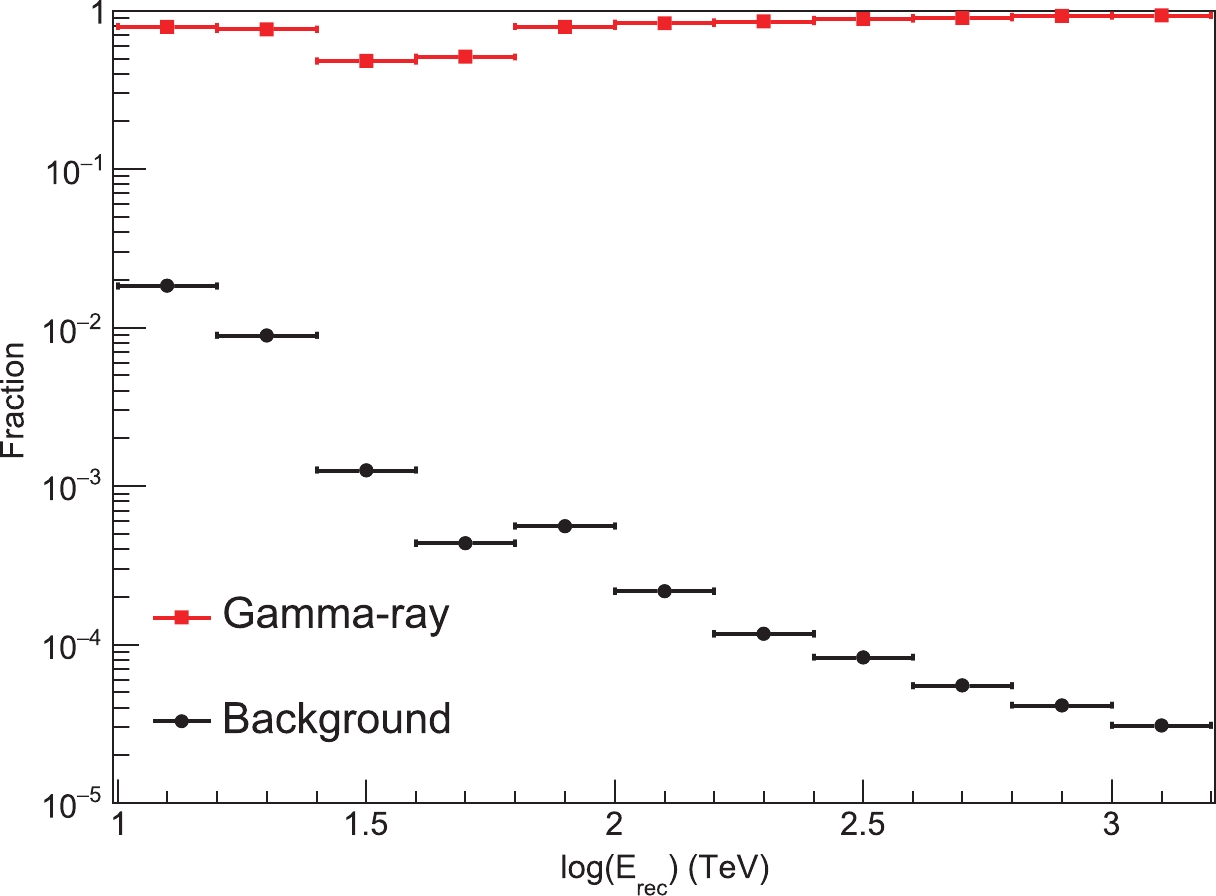
Figure 10. (color online) Survival fraction of γ-ray (according to simulation) and cosmic ray background events (according to observational data) in different energy bins after the discrimination cuts.
It is worth noting that these cuts are optimized for point-like sources. The rejection power can be improved using stricter cuts. For example, if the survival fraction for γ-ray showers were restricted to 60%, the rejection power for cosmic rays would be better than 2
$ \times $ 10$ ^{4} $ at energies above 100 TeV. -
The effective area of the KM2A for detecting γ-ray showers is calculated using the simulation. It is energy and zenith angle dependent. Figure 11 shows the effective areas at four zenith angles
$ \theta = 10^{\circ} $ ,$ 30^{\circ} $ ,$ 40^{\circ} $ and$ 50^{\circ} $ . The data quality and γ-ray/background discrimination cuts have been applied here. The effective area increases with energy and gradually reaches a constant value at energies above 30 TeV for zenith angles less than$ 30^{\circ} $ . The effective area is about 3$ \times $ 10$ ^{5} $ m$ ^{2} $ at 20 TeV for a zenith angle of 10$ ^{\circ} $ .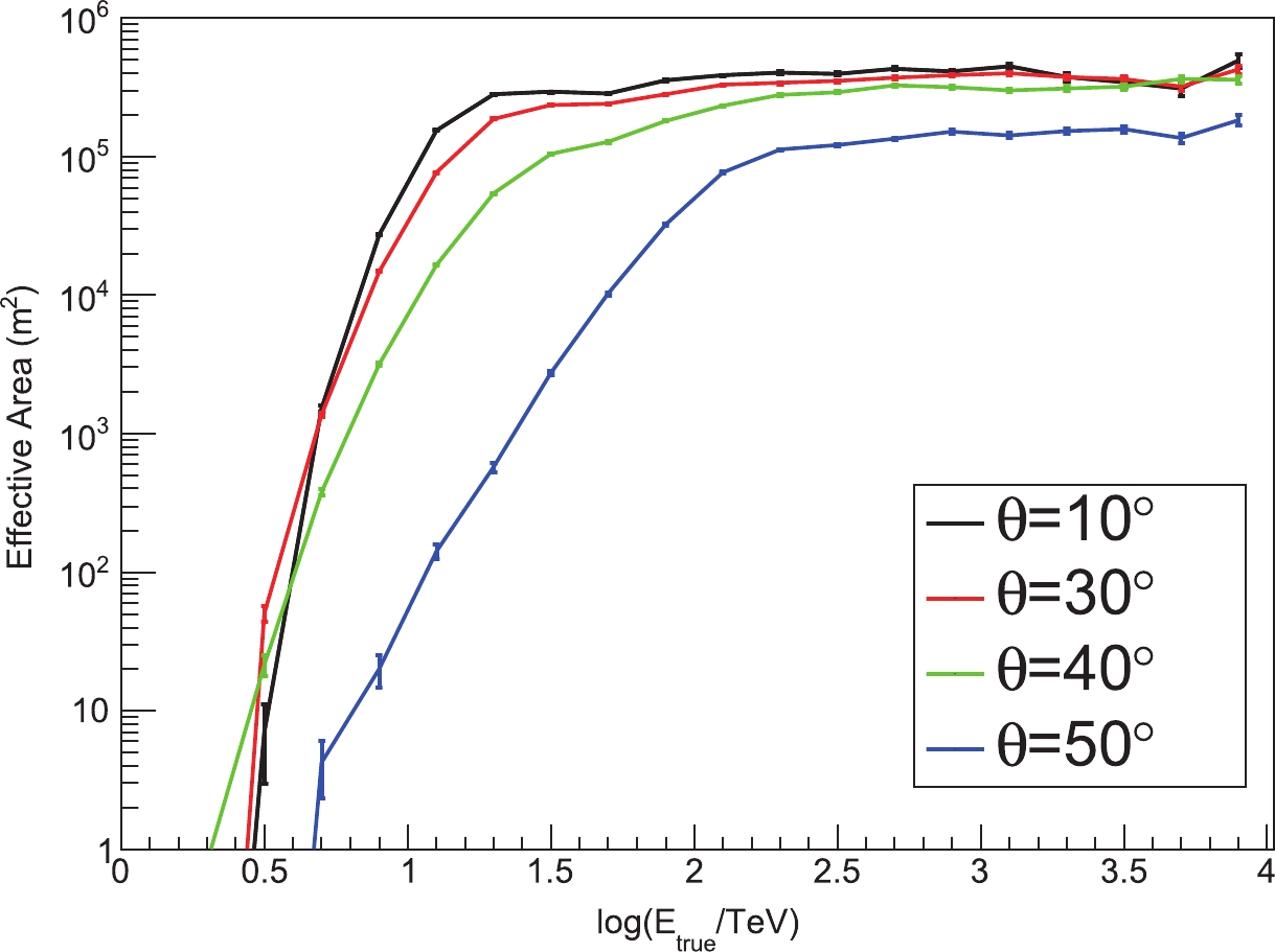
Figure 11. (color online) Effective area of the KM2A for γ-ray showers at four zenith angles after applying the data quality and γ-ray/background discrimination cuts.
-
For the analysis presented in this paper, only events with zenith angles less than 50 degrees and energies above 10 TeV are used. The data quality cuts and the γ-ray/background discrimination cuts discussed in the previous section are applied. The data sets are divided into five groups per decade according to the reconstructed energy. For the data set in each group, the sky map in celestial coordinates (right ascension and declination) is divided into a grid of
$ 0.1^{\circ}\times0.1^{\circ} $ pixels which are filled with the number of the detected events according to their reconstructed arrival direction (event map). To obtain the excess of$ \gamma $ -induced showers in each pixel, the “direct integration method” [28] is adopted to estimate the number of cosmic ray background events in the bin. The direct integration method uses events with the same direction in local coordinates but different arrival times to estimate the background. In this work, we integrated 24 hours of data to estimate the detector acceptance for different directions. The integral acceptance combined with the event rate is used to estimate the number of background events in each pixel (background map). This method is widely used for the ARGO-YBJ [3] and HAWC [5] experiments.The background map is then subtracted from the event map to obtain the source map which is used to extract the γ-ray signal from any specific source. The events in a circular area centered on each pixel within an angular radius of the KM2 point spread function (PSF) are summed. The number of excess events centered on the Crab Nebula in each energy bin is used to estimate its γ-ray spectrum.
-
The LHAASO-KM2A data used in this analysis were collected from 27th December 2019 to 28th May 2020. As this was the beginning of operation, some detectors still needed debugging during this period. To obtain a reliable data sample, some quality selections have been applied according to the data status. The main selection is to require the number of live EDs
$ >2100 $ and number of live MDs$ >500 $ . Figure 12 shows the daily duty cycle after these selections. The average duty cycle is 87.7% during this period. The total effective observation time is 136.0 days. With a trigger rate of about 900 Hz, the number of events recorded by KM2A is 1.0$ \times $ 10$ ^{10} $ . After the data quality cuts and the γ-ray/background discrimination cuts, the number of events used in this work is 6$ \times $ 10$ ^{7} $ .
Figure 12. (color online) Daily duty cycle of 1/2 KM2A operation during the period from December 2019 to May 2020.
Using these data, the sky is surveyed in the region with declination within
$ -15^{\circ}< $ Dec$ <75^{\circ} $ . In order to extract a smooth significance map, the likelihood method (see Eq. 2.5 in Ref. [29]) is adopted to estimate the significance of the$ \gamma $ -ray signal. A 2-dimensional Gaussian is used to approximately describe the PSF of the KM2A detector. The width of the Gaussian is set to be$ \sigma_{R} $ =$ \phi_{68} $ /1.51, which is obtained using the simulation sample. A likelihood ratio test is performed between the background-only model and the one-source model. The test statistic (TS) is used to estimate the significance S =$ \sqrt{{TS}} $ . This method is realized using the MINUIT package. The pre-trial significance distribution in the whole sky region at energies above 25 TeV is shown in Fig. 13. The distribution closely follows a standard Gaussian distribution, except for a tail with large positive values, due to excesses from γ-ray emission from the Galactic Plane including the Crab Nebula. After excluding the Galactic region with latitude$ |b|<12^{\circ} $ , the distribution, with a mean value of −0.05 and$ \sigma $ = 1.007, closely follows a standard normal distribution.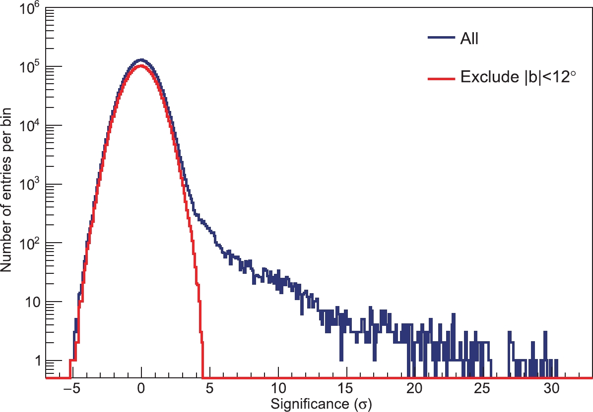
Figure 13. (color online) Pre-trial significance distribution of events with E
$_{\rm{rec}}>$ 25 TeV for the whole KM2A sky region (blue) and the portion of the sky outside the Galactic Plane region with$|b|>12^{\circ}$ (red), which represents diffuse background events.Focusing on the Crab Nebula region, a clear signal is observed in different energy ranges, i.e., 19.2
$ \sigma $ at 10-25 TeV, 28.0$ \sigma $ at 25-100 TeV and 14.7$ \sigma $ at$ > $ 100 TeV (see Fig. 14). A signal with such a level of significance allows us to estimate the pointing error of the detector, the angular resolution for γ-ray showers, and the γ-ray spectrum from the Crab Nebula.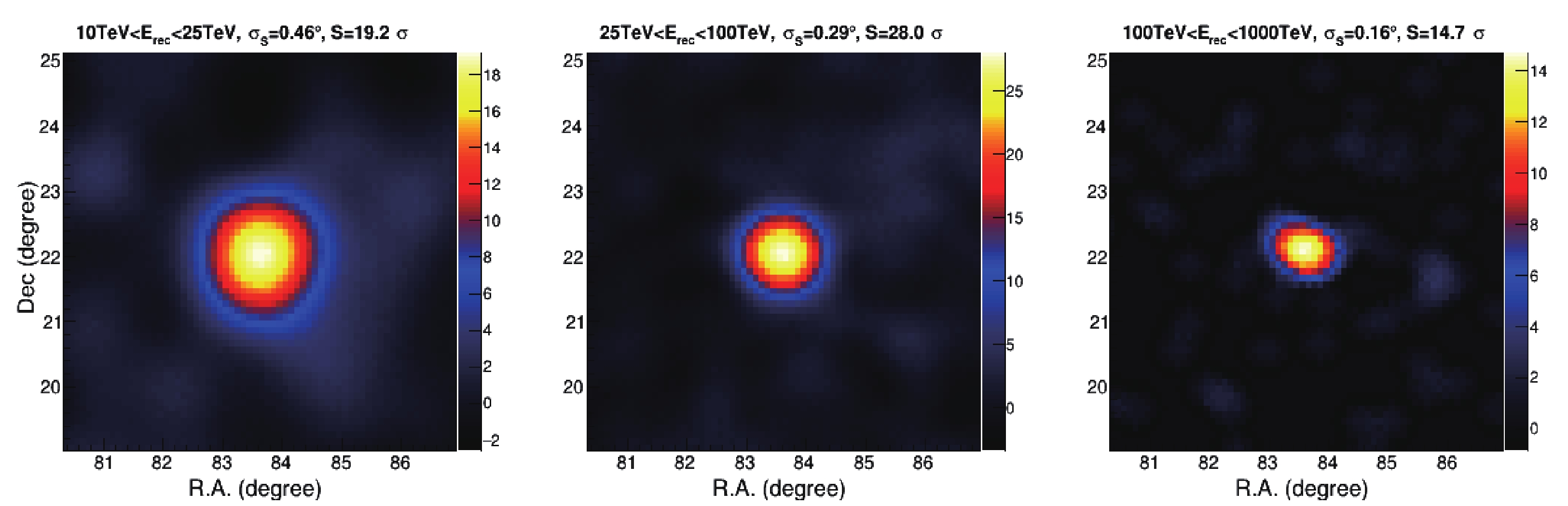
Figure 14. (color online) Significance maps centered on the Crab Nebula at three energy ranges.
$\sigma_{{S}}$ is the sigma of the 2-dimension Gaussian taken according to the PSF of KM2A. The color represents the significance. S is the maximum value in the map. -
To estimate the position of the γ-ray signal around the Crab Nebula direction at different energy bins, a 2-dimensional Gaussian is used to fit the event excess map. The positions obtained, in right ascension (R.A.) and declination (Dec) relative to the known Crab position (R.A. = 83.63
$ ^{\circ} $ , Dec = 22.02$ ^{\circ} $ , J2000.0 epoch) are shown in Fig. 15. The last energy point in Fig. 15 is obtained using the bins with 100 TeV$ <{{E}}_{\rm{rec}}< $ 1 PeV. When a constant value is used to fit the positions at all energies, we obtain$ \Delta $ R.A. = −0.024$ ^{\circ}\pm $ 0.016$ ^{\circ} $ ,$ \Delta $ Dec = 0.035$ ^{\circ}\pm $ 0.014$ ^{\circ} $ .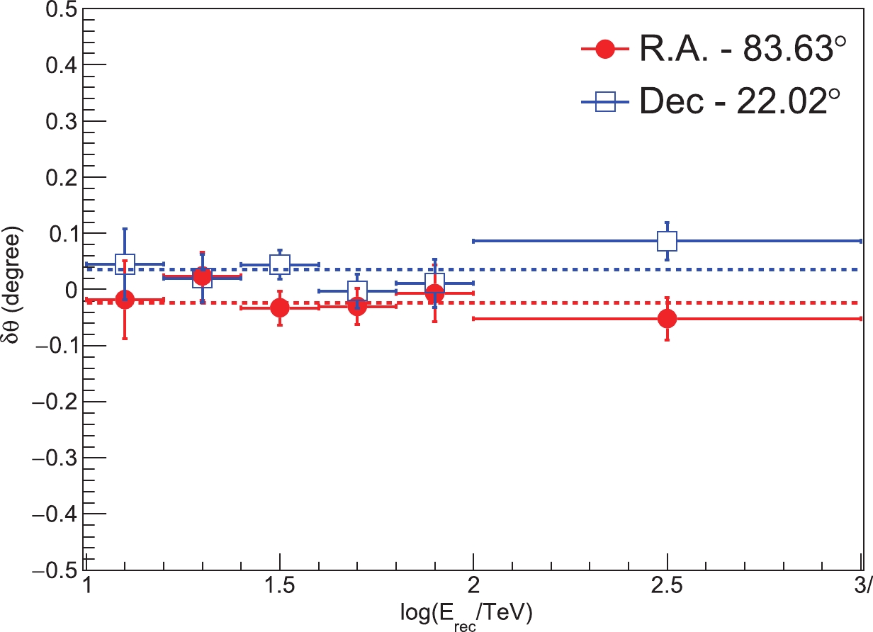
Figure 15. (color online) The centroid of the significance map around the Crab Nebula in R.A. and Dec directions as a function of energy. The dashed lines show constant values that fit the centroid for all energies.
The Crab Nebula can be observed by KM2A for about 7.4 hr per day with a zenith angle less than 50
$ ^{\circ} $ , culminating at 7$ ^{\circ} $ . The observation time for zenith angle less than 30$ ^{\circ} $ is 4.3 hr per day. To check for a possible systematic pointing error at large zenith angles, the observation of the Crab Nebula at zenith angles higher than 30$ ^{\circ} $ is analyzed separately. At energies$ > $ 25 TeV, the achieved significance is 12$ \sigma $ , and the obtained position relative to the known Crab position is$ \Delta $ R.A. = −0.073$ ^{\circ}\pm $ 0.042$ ^{\circ} $ ,$ \Delta $ Dec = 0.074$ ^{\circ}\pm $ 0.032$ ^{\circ} $ . This result is roughly consistent with that obtained using all data within statistical errors.According to these observations of the Crab Nebula, the pointing error of KM2A for γ-ray events can be demonstrated to be less than 0.1
$ ^{\circ} $ . -
According to a recent HESS measurement [30], the intrinsic extension of TeV γ-ray emission from the Crab Nebula is about 0.014
$ ^{\circ} $ . Compared with the PSF of the KM2A detector, the intrinsic extension is negligible. Therefore, the angular distribution of γ-rays detected by KM2A from the Crab Nebula should be mainly due to the detector angular resolution. Figure 16 shows the measured angular distribution in KM2A data in two energy ranges. The solid-angle density of recorded events in the vicinity of the Crab Nebula is shown as a function of$ \theta^{2} $ , where$ \theta $ is the angle to the Crab direction. The distribution is generally consistent with the angular resolution obtained using MC simulations. For each energy bin, a Gaussian function is used to fit the angular distribution shown in the left-hand and middle panels of Fig. 16. The resulting$ \sigma_{\rm PSF} $ from Crab data is consistent with simulations, as shown in the right-hand panel of Fig. 16.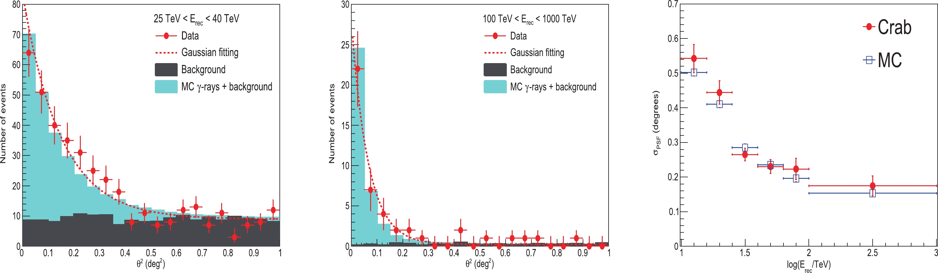
Figure 16. (color online) Distribution of events as a function of the square of the angle to the Crab direction for both experimental data and MC simulation. Two energy ranges, i.e., 25
$-$ 40 TeV (left) and 100$-$ 1000 TeV (middle) are shown. The right-hand panel shows the$\sigma_{\rm PSF}$ as a function of energy. -
The γ-ray flux from the Crab Nebula is estimated using the number of excess events (N
$ _{\rm{s}} $ ) and the corresponding statistical uncertainty ($ \sigma_{{N_{\rm s}}} $ ) in each energy bin. The γ-ray emission from the Crab Nebula is assumed to follow a power-law spectrum f(E)$ = {{J}}\cdot{{E}}^{\alpha} $ . The response of the KM2A detector was simulated by tracing the trajectory of the Crab Nebula within the FOV of KM2A. The best-fit values of J and$ \alpha $ are obtained by minimizing a$ \chi^2 $ function for 7 energy bins:$ {\chi ^{\rm{2}}}{\rm{ = }}\sum\limits_{{{i = 1}}}^{\rm{7}} {{{\left( { {\frac{{{{{N}}_{{{\rm{s}}_{{i}}}}}{\rm{ - }}{{{N}}_{{\rm{M}}{{\rm{C}}_{{i}}}}}({{J}},\alpha )}}{{{\sigma _{{{N}}_{{\rm{s}}_{{i}}}}}}}} } \right)}^{\rm{2}}}}. $

(8) Since the fit of the spectrum is forward-folded, the biases and energy resolution in the energy assignments are taken into account. The influence coming from the asymmetry in energy resolution shown in Fig. 8 can be neglected. The resulting differential flux (TeV
$ ^{-1} $ cm$ ^{-2} $ s$ ^{-1} $ ) in the energy range from 10 to 250 TeV is:$ \begin{aligned}[b] {{f}}({{E}}){\rm{ = }}&({\rm{1}}.{\rm{13}} \pm {\rm{0}}.{\rm{0}}{{\rm{5}}_{{\rm{stat}}}} \pm {\rm{0}}.{\rm{0}}{{\rm{8}}_{{\rm{sys}}}}) \times {\rm{1}}{{\rm{0}}^{{\rm{ - 14}}}}\\& {\left( { {\frac{E}{{20\;{\rm TeV}}}} } \right)^{ - 3.09 \pm {{0.06}_{\rm stat}} \pm {{0.02}_{\rm sys}}}}. \end{aligned} $

(9) The
$ \chi^{2} $ of the fit is 1.8 for 5 degrees of freedom, which favors a pure power-law description of the spectrum. The SED is shown in Fig. 17 and is also listed in Table 1. The SED obtained in this work is in agreement with previous observations by other detectors, such as HEGRA [7], HAWC [5] and Tibet AS-$ \gamma $ [6]. The discrepancy between this result and that measured by H.E.S.S. [8] and MAGIC [9] in the overlapping region may be due to their large systematic uncertainties at the highest energy region.log(E $_{\rm{rec}}$ /TeV)

E $_{middle}$ 

N $_{on}$ 

N $_{b}$ 

Differential Flux (TeV) (TeV $^{-1}$ cm

$^{-2}$ s

$^{-1}$ ))

[1.0, 1.2] 12.6 10810 9620 (4.52 $\pm$ 0.40)

$\times$ 10

$^{-14}$ 

[1.2, 1.4] 20.0 2513 1902 (1.13 $\pm$ 0.09)

$\times$ 10

$^{-14}$ 

[1.4, 1.6] 31.6 294 81 (2.98 $\pm$ 0.24)

$\times$ 10

$^{-15}$ 

[1.6, 1.8] 50.1 91 9.3 (6.64 $\pm$ 0.78)

$\times$ 10

$^{-16}$ 

[1.8, 2.0] 79.4 47 4.0 (1.43 $\pm$ 0.23)

$\times$ 10

$^{-16}$ 

[2.0, 2.2] 126 21 0.50 (4.05 $\pm$ 0.91)

$\times$ 10

$^{-17}$ 

[2.2, 2.4] 200 7 0.11 (8.0 $_{-3.2}^{+3.8}$ )

$\times$ 10

$^{-18}$ 

Table 1. Energy and differential flux as shown in Fig. 17
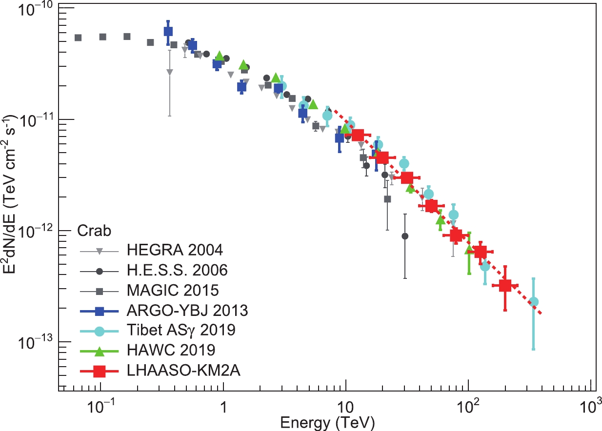
Figure 17. (color online) Spectrum of the Crab Nebula measured by KM2A, in red, with spectra measured by other experiments, in various colors as indicated in the legend. The dotted line indicates the best-fit result using a power-law function. References for other experiments are: HEGRA [7], H.E.S.S. [8], MAGIC [9], ARGO-YBJ [3], HAWC [5], Tibet AS-
$\gamma$ [6]. -
The systematic errors affecting the SED have been investigated by studying the variation of the Crab Nebula spectrum under various assumptions. During the period of interest, a few percent of detector units were being debugged. The number of operating units varied with time. A typical layout is taken into account in the detector simulation to mimic the status of the array. The uncertainty is estimated by using different configurations in the detector simulation. The variation of detector number affects the γ-ray/background separation, while the impact on γ-rays is weaker than on the background. The maximum variation in flux introduced by detector layout is less than 2%. The main systematic error comes from the atmospheric model used in the Monte Carlo simulations. The atmospheric density profile in reality always deviates from the model provided in Ref. [15], due to seasonal and daily changes. According to the variation of event rate during the operational period, the total systematic uncertainty is estimated to be 7% for the flux and 0.02 for the spectral index.
-
Using the first five months of data from the KM2A half-array, a standard candle at very high energy − the Crab Nebula − has been observed to investigate the detector performance and corresponding data analysis pipeline for γ-rays. The statistical significance of the γ-ray signal from Crab Nebula is 28.0
$ \sigma $ at 25-100 TeV and 14.7$ \sigma $ at$ > $ 100 TeV. The γ-ray angular distributions around the source are fairly consistent with the point spread function obtained by simulations. According to measurement of the centroids of the significance maps of the Crab Nebula at different energies, the pointing error of KM2A is found to be less than 0.1$ ^{\circ} $ . The spectrum from 10 TeV to 250 TeV can be fitted well with a power-law function with a spectral index of$ 3.09\pm0.06_{\rm stat}\pm 0.02_{\rm sys} $ . This result is quite consistent with previous measurements by other experiments. The overall systematic error of KM2A on spectral measurement is estimated to be 7% in flux and 0.02 in spectral index.The KM2A data analysis pipeline presented in this work is not specifically designed for the Crab Nebula but is also generally useful for surveying the whole sky in the range of declination from −15
$ ^{\circ} $ to 75$ ^{\circ} $ and the corresponding measurements for source morphology and energy spectra. This opens a new window of γ-ray astronomy above 0.1 PeV. A new era of ultrahigh-energy γ-ray astronomy foreshadows a fruitful future for fundamental discoveries. -
The authors would like to thank all staff members who work at the LHAASO site above 4400 meters above sea level year-round to maintain the detector and keep the electrical power supply and other components of the experiment operating smoothly. We are grateful to the Chengdu Management Committee of Tianfu New Area for their constant financial support of research with LHAASO data.
Observation of the Crab Nebula with LHAASO-KM2A − a performance study
- Received Date: 2020-10-13
- Available Online: 2021-02-15
Abstract: A sub-array of the Large High Altitude Air Shower Observatory (LHAASO), KM2A is mainly designed to observe a large fraction of the northern sky to hunt for γ-ray sources at energies above 10 TeV. Even though the detector construction is still underway, half of the KM2A array has been operating stably since the end of 2019. In this paper, we present the KM2A data analysis pipeline and the first observation of the Crab Nebula, a standard candle in very high energy γ-ray astronomy. We detect γ-ray signals from the Crab Nebula in both energy ranges of 10


 DownLoad: