A minimisation method for accurate position-determination using a position-sensitive Schottky cavity doublet

The origin of the heavy elements is a long-standing question in nuclear astrophysics that relies on measurement of short-lived rare radio-isotopes to constrain the predictions of various mass models [1, 2]. The masses of these isotopes are regularly measured at storage rings using the isochronous mode, which has become the dominant method used to achieve high precision in short timeframes (<50 ms). Due to the nature of isochronicity, achieved when the Lorentz factor of the particle γ is equal to the transition energy of the ring $ \gamma_t $, it can only be truly obtained for a single species of particle at a certain energy - usually the reference ion. All other species will have a greater deviation from $ \gamma=\gamma_t $ which increases as the mass to charge ratio diverges from that of the reference. In order to adjust for this deviation a correction is employed, often by relating the magnetic rigidity $ B\rho $ to either the circulating particle's circumference (C) or its time of flight (ToF). The Cooler Storage Ring (CSRe) in Lanzhou recently employed a $ B\rho $-ToF correction using two in-ring ToF detectors to achieve an impressive mass precision of ≈ 5 keV [3, 4]. They utilised an iterative fit of the $ B\rho $ function and careful analysis to reduce systematic errors such as magnetic field drift during analysis.

The Rare Radio-Isotope Ring (R3) at RIKEN, Japan is a dispersive ring that uses a unique single particle injection method [5]. Here, a position-sensitive detector ahead of the ring in the BigRIPS fragment separator is used to correct the momentum spread [6]. A disadvantage of the current method is that it assumes the momentum of the particle measured at F5 (Figure 1) will be preserved after passing through the fragment separator, which contains various detectors, and after being kicked by an injection magnet into the storage ring - a discrepancy found recently between the expected $ B\rho $ calculated at F5 and that measured by an NMR probe inside the ring [6] challenges this assumption. Moreover, momentum information is only collected once which results in relatively low statistics for rarer ions which are the main focus of mass measurements at R3. These factors contribute to the mass measurement uncertainty which is over one order of magnitude larger than the results from CSRe [7].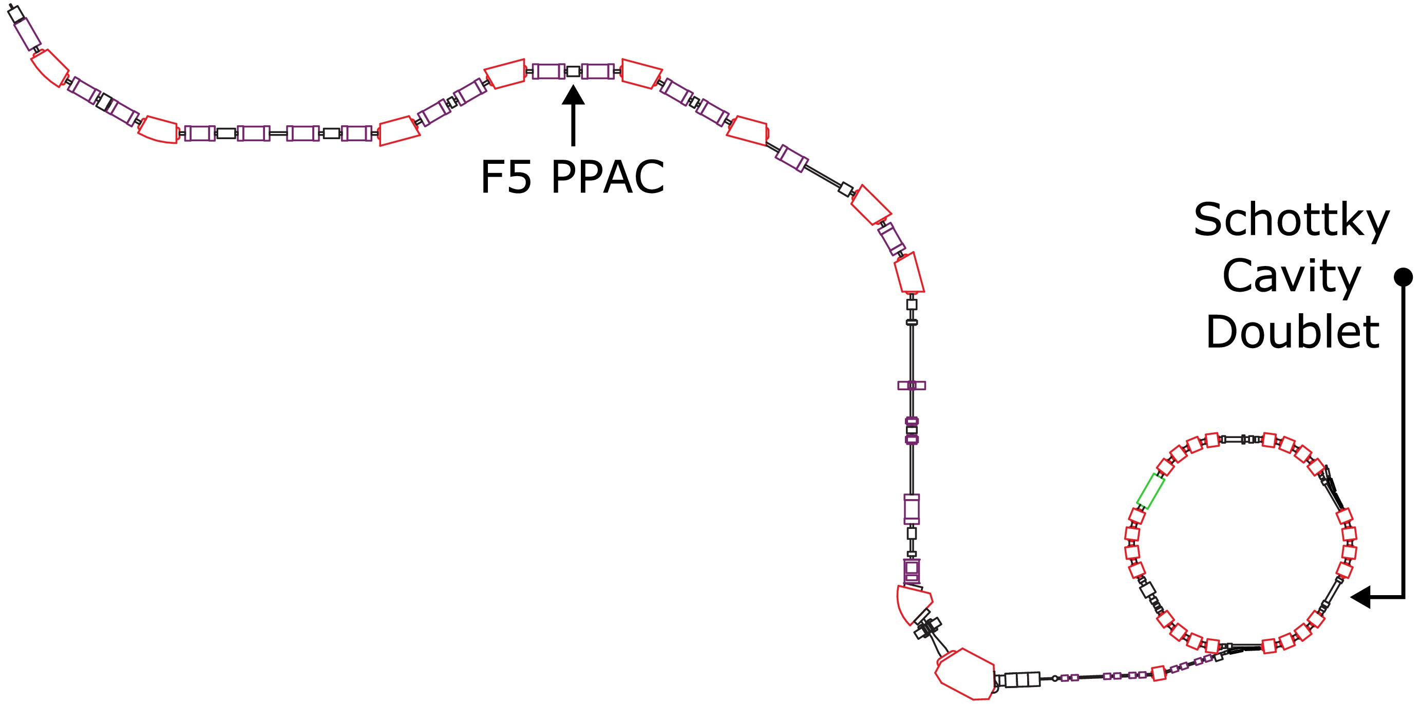

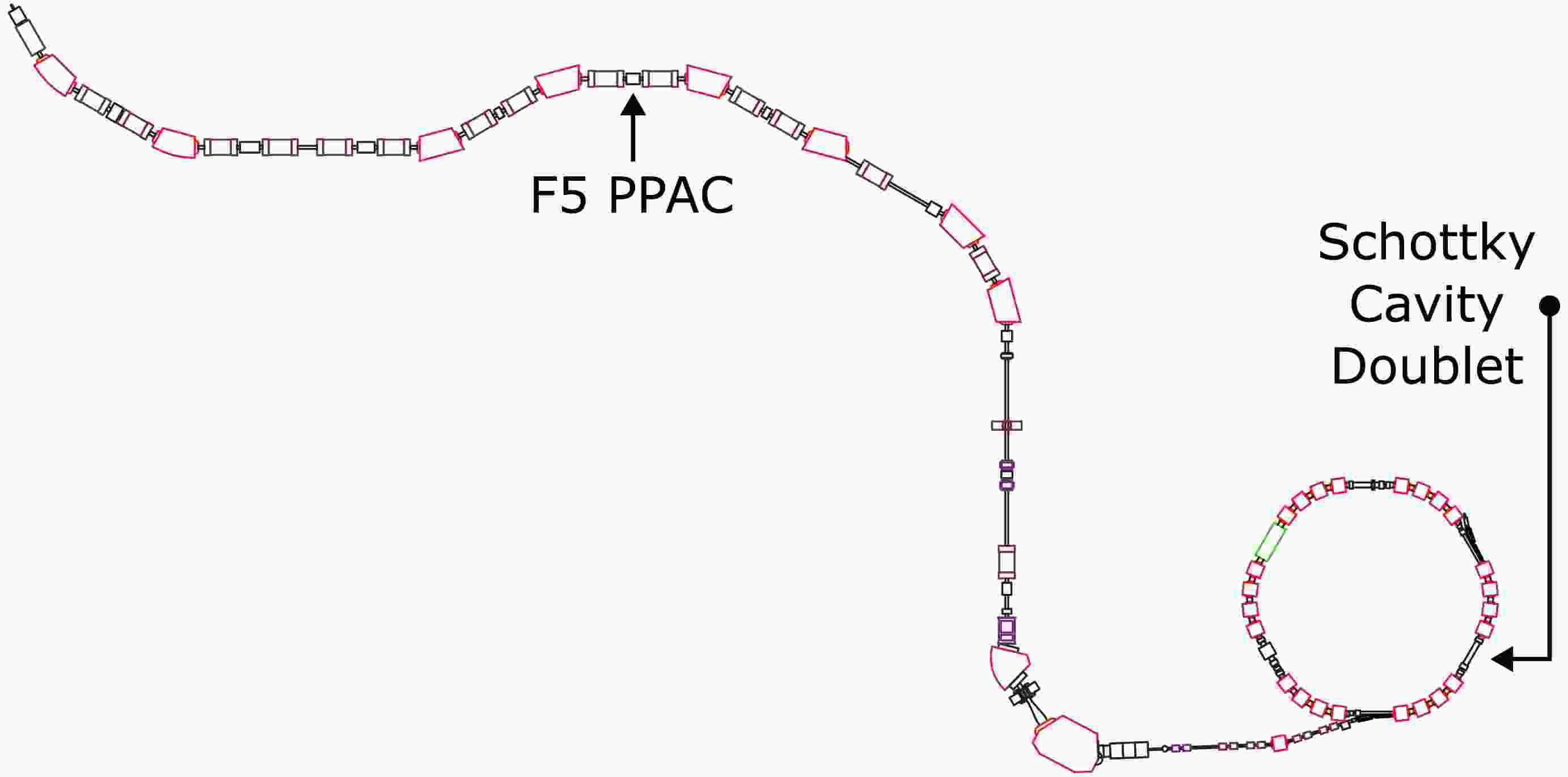
Figure 1.  (color online) BigRIPS fragment separator beam line to the R3 storage ring. The position-sensitive PPAC at F5 makes the measurement of the x-position for the current $ B\rho $ correction method.

In order to provide accurate information about the momentum distribution inside the ring, a position-sensitive Schottky Cavity Doublet (SCD) has been installed at R3 to collect position information. A $ B\rho $ correction can be performed using this data and mass determination can be carried out using the correlation matrix method (CMM) [8, 9] or the $ B\rho $-C method [6, 10]. In this paper we will focus on the CMM as the end goal. Importantly, the large momentum acceptance at R3 allows injected isotopes to populate a large portion of the horizontal range of the ring's beam-pipe. This complete data set lets us identify and parametrise factors that contribute to systematic errors. Minimising these parameters then results in a large reduction in the systematic uncertainty. Another noteworthy advantage is that this method allows the removal of detectors upstream that introduce unwanted particle loss due to charge-change interactions. This is particularly important for future measurements of high Z isotopes, such as the accepted proposal to measure neutron rich ^216-220Pb isotopes (NP2412-RIRING09).

The SCD consists of a cylindrical reference cavity and an elongated elliptical cavity. An electromagnetic field is excited inside each by a current induced from ions passing through periodically. The power stored in the cavity is expressed as

where γ is the Lorentz factor, q is the charge, $ f_{\text{rev}} $ is the revolution frequency and η is the coupling factor

where $ R_l $ is the load resistance and $ \left(\dfrac{R_{sh}}{Q}\right)Q $ is the shunt impedance [12]. The power is coupled out using a magnetic loop and processed with a Fourier transform to produce a frequency signal. The elliptical cavity has an offset beam pipe which covers the decreasing electromagnetic field gradient, introducing a horizontal position dependence into the power of the cavity's signal. Relative to the cylindrical cavity, the power of the elliptical cavity is scaled by a factor $ F(x) $ depending on its position according to an R/Q (normalised shunt impedance) map, such that

where ell and cyl denote the elliptical and cylindrical cavities and $ F(x) $ was calculated by a simulation in ref. [11]. Non-position dependent factors can be removed by a division of the signals to create the normalised power,

Both cavities exploit the monopole mode for the highest sensitivity and their simulated field distributions are pictured in Figure 2. Readers desiring a full description of resonant Schottky cavity theory are directed to references [10−18].

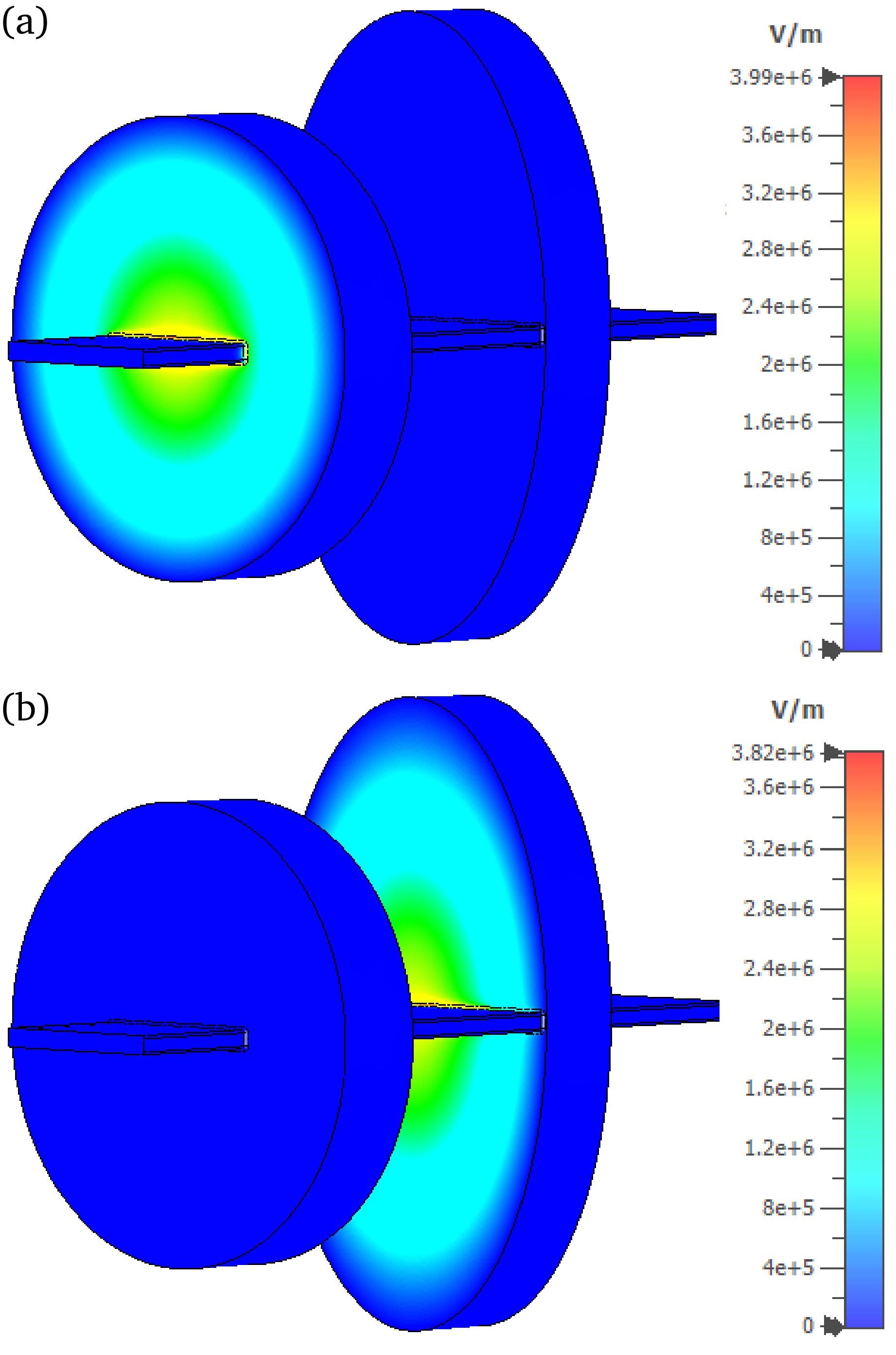
Figure 2.  (color online) A simulation from ref. [11] showing the electromagnetic field distribution of the monopole mode inside both cavities. (a) shows field of the cylindrical cavity and (b) shows that of the elliptical cavity. The beam pipe of the elliptical cavity is offset to cover the decreasing gradient of the field.

The goal of the SCD mass measurement method is to associate each particle's frequency $ f_i $ with a position $ x_i $, where i denotes a particle from a single injection. These pairs can then be input into the CMM to calculate the mass. This is a two-step process comprised of an initial position determination and a minimisation acting as a second-order correction to reduce the systematic uncertainty.

Each particle generates a frequency signal with frequency $ f_i $ and an associated power $ P_i $. From $ P_i $, the related $ x_i $ is found using the $ F(x) $ relation. Logically, each $ f_i $ is then related to an $ x_i $ through $ P_i $ as described in ref. [19]. It may be necessary to introduce an additional factor a between the $ f_i-P_i $ and $ P_i-x_i $ relations, which can be determined after parametrisation. This initial determination is limited by the resolution of the R/Q map, therefore in the second step one can minimise the fit of $ P_i $ to $ x_i $ to improve the accuracy of $ F(x) $.

The initial function fitted to the normalised power for each isotope is

where $ F(x) $ can be assumed to be transversally linear in the first approximation. It is likely that a linear fit will not provide sufficient precision, therefore after evaluating the initial fit, it may be appropriate to use a second order polynomial or others where appropriate. The amount of additional constants in Equation 5 can be dynamic in order to characterise any parameters that introduce systematic uncertainties.

For example, if an isotopic dependency existed, the fit of Equation 5 for both isotopes can be compared to identify their relationship. This can be parametrised and appended as an additional correction. The strength of this method is complimented by the population of data across the entire momentum acceptance of R3, provided naturally due to its dispersive nature. A final consideration can be made to the power response of the cavity over the entire experimental period. This will reveal the electromagnetic field fluctuation of R3's bending magnets which can be fitted and corrected.

Due to the resonant nature of the cavity, the amplitude of the its signal is at its maximum at the resonant frequency, $ f_{\text{res}} $ and decreases rapidly as the differential from this frequency increases. This means that the amplitude of the signal is not solely dependent on $ F(x) $, but also $ df = f_{\text{res}} - f_i $; this additional dependence should be corrected. The shape of the resonant peak can be seen in the thermal noise, which takes the form of a Lorentzian distribution about $ f_{\text{res}} $. Its area is dependant on the Q value, which is different for each cavity, meaning the amplification by resonance is different for both cavities. In addition, the resonant frequency may be misaligned as it is adjusted manually with tuners. Such a situation is illustrated in Figure 3. These factors mean that a simple division of the elliptical cavity's signal with the cylindrical reference cavity will result in an incorrect determination of the magnitude of the normalised signal.

Figure 3.  (color online) Power vs frequency of mock background signals from each cavity. The shape of each is different and may be misaligned in the frequency space.

Since the resonant peak is well defined by the thermal noise, one may normalise the signals by finding the amplification factor between the noise signal for each cavity. A standard fitting algorithm is easily confused by the presence of frequency peaks, therefore we will use the Bayesian reweighted penalized least squares (BrPLS) method which was recently developed specifically for analysis of Schottky spectra [20, 21]. Thus, a fit of the background $ G(f) $ can be used to normalise the power signal $ P(f) $ such that the normalised power will become

Naturally, this normalisation will take place before the fitting of Equation 5.

Once $ x_i $ for each injection has been found, a $ B\rho $ correction can be applied to correct the momentum spread before the $ f-x $ pairs are input to the CMM. The average power $ P_{\text{avg}} $ and frequency $ f_{\text{avg}} $ of each species can be determined by a Gaussian fit of the summation of the individual Schottky spectra for each species. Using the $ F(x) $ relation, we can find $ x_{\text{avg}} $ from $ P_{\text{avg}} $ and fit it against the $ f_{\text{avg}} $. Assuming a linear fit, the corrected frequency is calculated by subtracting the average position from each $ x_i $ such that

where m and c are the gradient and intercept of the linear fit.

There are a number of conditions that are favourable for a definitive pilot test with the SCD. Data on the calibration run should be collected using a primary beam to maximise statistics, using a species previously measured in R3 which allows a comparison of the mass resolution with previous techniques. Furthermore, the beam should have sufficiently high charge to create a strong single particle signal for the resonant cavity, similar to that of the medium to high Z elements we wish to measure in the future. The dispersion of the ring should be sufficient for performing the minimisation method, such that a single particle's momentum spread fills a large portion of the detector's momentum acceptance, and to ensure a detectable differential in Schottky power. Considering beam availability and the factors above, ⁷⁶Zn was chosen as the reference isotope. It is not a primary beam but the intensity will be adequate for the pilot experiment (≈1000 cps).

A simulation was performed in CERN's MAD-X [22] to estimate the dispersion and horizontal position inside the ring. The simulation was performed with the PTC module [23, 24] which employs symplectic calculations to retain high accuracy over thousands of turns. The code can be found on GitHub [25]. First, we show the newly calculated beta functions and dispersion for R3 in Figure 4. These were originally calculated in 1987 for the TARN-II ring, the origin of R3's dipole magnets [26].

Figure 4.  (color online) Beta functions and horizontal dispersion for a 200 MeV/u beam. Shown is all six sectors of the R3 lattice starting and ending in the center of a straight section.

Next, the dispersion of the ring was confirmed by recording the position of particles as they passed a non-destructive monitor, placed at the installed location of the SCD. The starting point is arbitrary; we chose to initiate each particle at the end of the straight section, parallel to the injection septa. The initial X-position distribution was Gaussian, with a 70 mm standard deviation corresponding to the injection septum horizontal acceptance and a horizontal momentum gaussian distribution of 0.2%. The momentum acceptance was covered by different $ \delta p/p $ settings. On each setting, 1000 particles were simulated with each particle making 10000 turns of the ring, creating a histogram of the positions recorded at the SCD. This was fitted with a Gaussian and the mean value and its standard deviation for each setting can be seen in Figure 5. A linear fit finds the dispersion to be 66.9 mm/% which corresponds to the designed value [5] and is sufficient for the minimisation method.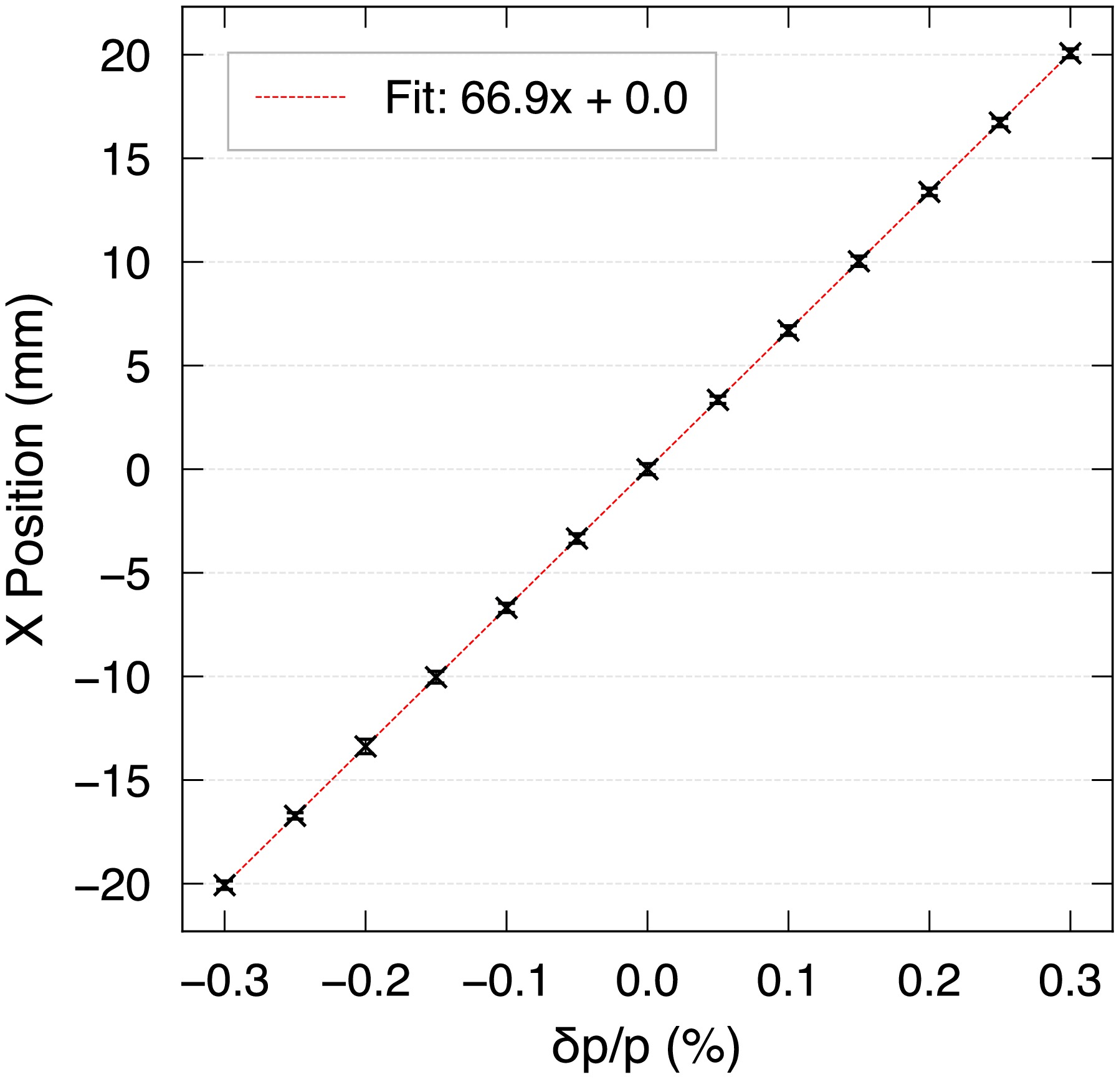

Figure 5.  (color online) Simulation of the x-position dependency on relative change in momentum at the installed position of the Schottky detector inside R3 using MADX.

The horizontal distribution inside R3 was also verified using the LISE++ simulation software [27]. This was checked at the center of the kicker magnet pre-injection, however the distribution should be unchanged post injection. The results are shown in Figure 6. Across the central $ \pm $50 mm range of the beam-pipe there is good coverage of the momentum acceptance. It is desirable to cover a greater range to collect data for the minimisation method, therefore the energy of the beam should be changed slightly during the experiment. It can be reduced by $ dp/p= $0.15% by inserting either an aluminium foil or a PPAC detector upstream, or both in combination for a greater reduction.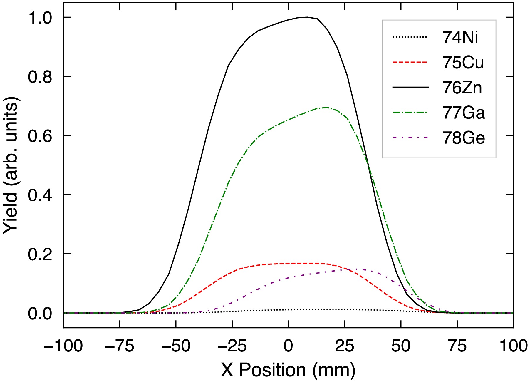

Figure 6.  (color online) Horizontal distribution at the kicker center after the partial pre-injection orbit of R3. Yield is normalised to the maximum yield of ⁷⁶Zn.

Finally, Table 1 lists the isotopes, their expected frequency peaks for the respected harmonic, their expected average position $ \bar{X}_{\text{exp}} $ and the power in each cavity $ P_{\text{cyl}} $ and $ P_{\text{ell}} $. The position was calculated in MADX and the associated power was estimated using the equation for an unloaded cavity (without considering coupling with external electronics),

Isotope	Harmonic	Expected Peak (MHz)	$ \bar{X}_{\text{exp}} $ (mm)	$ P_{\text{cyl}} $ (dBm)	$ P_{\text{ell}} $ (dBm)
74Ni	96	233.8	14	-134	-143
75Cu	95	235.4	6	-133	-138
76Zn	93	234.2	0	-133	-136
77Ga	92	235.2	-5	-132	-134
78Ge	90	233.2	0	-132	-135

Table 1.  Proposed fragments for the pilot test of the SCD.

where $ R_{sh}/Q $ is the value simulated for the cylindrical and elliptical cavities respectively from ref. [11] and the Q values are estimated to be $ Q_{\text{cyl}}=3000 $ and $ Q_{\text{ell}}=2300 $ for an unloaded cavity based on simulations. The thermal noise was calculated to be -180 dBm which means the estimated power in Table 1 will result in a good signal to noise ratio.

Other considerations include the recording time of data: it should be long to achieve a clear peak, but not so long as to significantly reduce the injection frequency - only one particle is stored at a time. Previous recordings using a Schottky detector in the R3 ring show stable orbits of approximately three seconds in vacuum [28] which can be used as the upper limit. For a reference isotope with relatively high intensity, it is suggested to use this maximum recording time for the pilot run for the best signal-to-noise ratio. Following this, the recording time can be optimised for high efficiency.

The simulated R/Q map is a limiting factor for precision, therefore it is of interest to calculate the R/Q map resolution required to match the precision of the F5 PPAC used for position determination. The PPAC has a resolution of ≈0.5 mm with a dispersion of 31.7 mm/% at F5 [29] which equates to a $ \delta p/p $ resolution of $ \sigma_{\text{PPAC}}\approx $0.0157%. This is the target resolution to be achieved at R3, which has dispersion of 66.9 mm/% according to the MADX simulation. The approximate linear gradient of the R/Q map calculated in [11] is ≈320 Ω/m. Assuming 320 Ω/m across the $ \pm $200 mm physical acceptance of the detector with a dispersion of 66.9 mm/%, one can find the gradient m of the impedance–$ \delta p/p $ relation. Then, using a change in momentum equal to the PPAC resolution, the uncertainty in impedance necessary to resolve this change in momentum is calculated as $ m \cdot \sigma_{\text{PPAC}} = $ 0.3 Ω.

This value is important as the uncertainty in this position measurement influences the precision of the F5 momentum correction and thus the precision of the mass measurement. The uncertainty in the impedance is represented by the uncertainty in $ F(x) $ in Equation 5, therefore the minimisation method described in section 2, should constrain the uncertainty of $ F(x) $ to $ \leq0.3\; \Omega $.

Comparing the PPAC and SCD resolutions allows for a cursory comparison of the two methods in terms of precision. Nonetheless, one must keep in mind that resolution is not the only metric in improvement of the mass measurement, which also depends on the degree of the accuracy of the single-pass momentum measurement at F5 in the case of the previous method.

A position-sensitive schottky cavity doublet was installed at R3 to improve the mass measurement accuracy. We detail the process for making a second order correction based on a beam with a large momentum distribution to categorise the parameter space of the cavity, showing with simulations that this distribution will be fulfilled. Characterisation of a wider range can be achieved by changing the beam energy. Lastly, in order to match the position resolution used in the current mass measurement method, the $ F(x) $ parameter of the power equation should aim for an uncertainty of $ \leq0.3\; \Omega $ to match the precision of the current mass measurement method. A beam-time has been approved to commission the detector which will allow us to check this value and compare the previous and proposed mass measurement methods. It is scheduled for 2025. If successful, this will not only improve accuracy but should also increase the yield and open up experiments with high Z beams. Switching to purely non-destructive measurements would also enable lifetime studies of the exotic nuclei of interest. A separate paper dedicated to the detector will be published in the future.