Investigating Interacting Dark Energy Models Using Fast Radio Burst Observations

Fast Radio Bursts (FRBs) are millisecond-duration radio transients characterized by unusually high dispersion measures (DMs), which serve as unique probes for studying the large-scale structure and evolution of the Universe [1]. Since their initial discovery by Lorimer et al. [2], more than 800 FRB events have been detected, with some precisely localized to host galaxies at cosmological distances [3, 4]. The DM value of an FRB reflects the cumulative column density of free electrons along the line of sight, which can be decomposed into contributions from the Milky Way ($ {\rm{DM}}_{\rm{MW}} $), the host galaxy ($ {\rm{DM}}_{\rm{host}} $), and the intergalactic medium (IGM) contribution ($ {\rm{DM}}_{\rm{IGM}} $) [5]. By disentangling these components, FRB observations provide valuable constraints on $ H_0 $ and $ \Omega_m $.

The cosmological utility of FRBs arises from the statistically significant correlation between the intergalactic medium's contribution to the dispersion measure ($ {\rm{DM}}_{\rm{IGM}} $) and redshift (z). Theoretical studies have shown that the mean value, $ \langle {\rm{DM}}_{\rm{IGM}} \rangle $, is directly related to the $ H_0 $ and the baryon density parameter ($ \Omega_b $) [6], In contrast, its distribution is notably affected by the inhomogeneity of baryon distribution in the intergalactic medium [7].

Recent studies have employed localized FRB data to measure the Hubble constant $ H_0 $ [8], and to test non-standard cosmological models, such as the $ R_h=ct $ universe [9]. Moreover, several investigations have examined the impact of the FRB redshift distribution on cosmological parameter constraints [10]. In addition, FRB observations have been used to explore the possibility that compact objects (COs) constitute a fraction of dark matter [11]. FRBs also serve as effective probes for studying the expansion history of the Universe and the physical properties of the intergalactic medium [12, 13]. Notably, by breaking parameter degeneracies inherent in Cosmic Microwave Background (CMB) data, FRB observations can significantly tighten constraints on the Hubble constant and dark energy parameters [14]. Furthermore, analysis of the CHIME/FRB catalog indicates that the observed redshift distribution of the FRB population cannot be fully explained by the star formation history (SFH) alone; instead, it requires the inclusion of a significantly delayed population or a mixture of populations to match the data [15−18]. These findings provide a crucial theoretical foundation for our study and strongly motivate the use of FRBs as novel cosmological tools to constrain models, including those involving interactions between dark energy and dark matter.

The physical nature of dark matter and dark energy, which together account for approximately 95% of the Universe's energy density, remains one of the most fundamental challenges in modern cosmology. Although the standard Lambda Cold Dark Matter (ΛCDM) model successfully describes the accelerated expansion of the Universe, basic questions remain unanswered, such as the “coincidence problem” — the phenomenon that the current energy densities of dark matter and dark energy are of the same order of magnitude despite their very different evolutionary histories. To address this coincidence problem related to the evolution of dark energy and dark matter, researchers have proposed the IDE model, which incorporates a non-gravitational coupling term, Q, to characterize the energy exchange between dark matter and dark energy. As extensively discussed in the literature [19−24], the IDE model assumes that the energy transfer between dark matter and dark energy can be described by an interaction term Q:

where $ \rho_x $ denotes the energy density of dark energy, $ \rho_m $ denotes that of dark matter, and $ p_x $ is the pressure of dark energy. The Hubble parameter H characterizes the expansion rate of the Universe. The time derivatives $ \dot{\rho}_x $ and $ \dot{\rho}_m $ describe the evolution of the energy densities with cosmic time. The interaction term Q quantifies the energy transfer between the two components: $ Q > 0 $ indicates a transfer of energy from dark energy to dark matter, whereas $ Q < 0 $ indicates the reverse. These equations ensure the conservation of the total energy density, as expressed by $ \dot{\rho}_{x} + \dot{\rho}_{m} + 3H(\rho_{x} + \rho_{m} + p_{x}) = 0 $.

This affects the integral form of $ \langle {\rm{DM}}_{\rm{IGM}} \rangle $. Meanwhile, the IDE model can also mitigate the Hubble tension to some extent [25]. Current constraints on dark energy and dark matter interactions derived from Type Ia supernovae (SNe Ia), the CMB, and baryon acoustic oscillations (BAO) remain weak, primarily due to parameter parsimony and limited redshift coverage [26−31]. Additionally, strong gravitational lensing time-delay measurements have emerged as a complementary tool to improve these constraints [32]. In contrast, FRB data can effectively probe high-redshift ($ z > 1 $) regions, extending beyond the observational limitations of SNe Ia and providing new constraints on the redshift evolution of dark interactions. Moreover, unlike quasar absorption lines or X-ray surveys, FRBs offer a more comprehensive census of ionized baryons, including the diffuse IGM, which constitutes approximately 80% of the total cosmic baryons [4].

Previous studies have demonstrated the potential of FRB simulations in constraining parameters of IDE models [33]. This study employs real FRB data to investigate three specific IDE models: $ \gamma_m $IDE, $ \gamma_x $IDE, and ξIDE. By imposing a relatively narrow Gaussian prior on $\Omega_m $, the $ \gamma_m $IDE model yields well-constrained posterior distributions for the remaining parameters. However, given the limitations of current observational data, the overall constraining power on cosmological parameters remains insufficient. To address this, we further analyze simulated FRB datasets and perform model selection using information criteria (IC), thereby establishing a more robust framework for future cosmological studies based on FRB observations.

In section 2, we provide a brief overview of DM measurements for localized FRBs. section 3 outlines the methodology and details the FRB samples employed in this study, including both observational and simulated data. In section 4, we conduct Markov Chain Monte Carlo (MCMC) analyses to constrain three IDE models. section 5 presents a theoretical interpretation and discussion of the results of the constraints. Finally, section 6 summarizes the main conclusions of the study.

The precise localization of a group of FRBs within their host galaxies enables the establishment of a correlation between the dispersion measure ($ {\rm{DM}}_{\rm{FRB}} $) and the redshift ($ {z_{{\rm{FRB}}}} $) of FRBs. $ {\rm{DM}}_{\rm{FRB}} $ represents the integral of the free electron density along the propagation path of an FRB signal and incorporates the effect of cosmic expansion on the path length by applying a redshift-dependent weighting factor of $ (1+z)^{-1} $.

From a physical perspective, the total $ {\rm{DM}}_{\rm{FRB}} $ can be decomposed into four primary components:

The $ {\rm{DM}}_{\rm{MW}}^{\rm{ISM}} $ component primarily originates from the interstellar medium (ISM) of the Milky Way and is typically estimated using Galactic electron density models such as the NE2001 model [34]. The $ {\rm{DM}}_{\rm{MW}}^{\rm{halo}} $ term, which represents the contribution from the Milky Way's halo, remains poorly constrained but is generally expected to fall within the range of 50-80 pc $ {\rm{cm}}^{-3} $. In the subsequent analyses of this paper, we adopt a fiducial value of $ {\rm{DM}}_{\rm{MW}}^{\rm{halo}} = 65 $ pc $ {\rm{cm}}^{-3} $ [35], noting that its variance and uncertainty are significantly smaller than those associated with $ {{\rm{DM}}_{\rm{IGM}}} $ and $ {{\rm{DM}}_{\rm{host}}} $, and can be effectively absorbed into the broader uncertainty budget of $ {{\rm{DM}}_{\rm{host}}} $ [3, 36, 37].

The $ {{\rm{DM}}_{\rm{IGM}}} $ component exhibits a pronounced dependence on redshift, as FRB signals traverse a considerable portion of the IGM during their propagation. The electron density in the IGM evolves with cosmic time, resulting in a substantial increase in $ {{\rm{DM}}_{\rm{IGM}}} $ with redshift. The redshift dependence of the mean $ {{\rm{DM}}_{\rm{IGM}}} $ can be quantitatively expressed by the following equation [38]:

where c is the speed of light, $ H_0 $ is the Hubble constant, $ \omega_b $ is the baryon density parameter, G is the gravitational constant, $ m_p $ is the proton mass, and $ f_d \simeq 0.84 $ [39] represents the fraction of cosmic baryons residing in diffuse ionized gas. The number of free electrons per baryon is given by $ \chi_e(z) = \frac{3}{4} \chi_{e,{\rm{H}}}(z) + \frac{1}{8} \chi_{e,{\rm{He}}}(z), $ where $ \chi_{e,{\rm{H}}}(z) $ denotes the ionization fraction of hydrogen, and $ \chi_{e,{\rm{He}}}(z) $ denotes that of helium. For redshifts $ z \lesssim 3 $, both hydrogen and helium are assumed to be fully ionized [40], such that $ \chi_{e,{\rm{H}}}(z) = 1 $ and $ \chi_{e,{\rm{He}}}(z) = 1 $, yielding $ \chi_e = \frac{7}{8} $. The function $ E(z') $ denotes the dimensionless Hubble parameter at redshift $ z' $, which is determined by the underlying cosmological model.

The probability distribution function (PDF) of $ {{\rm{DM}}_{\rm{IGM}}} $ is derived from a theoretical treatment of the IGM and the Galactic halo [35, 41].

Here, Δ denotes the ratio of $ {\rm{DM}}_{\rm{IGM}} $ to its mean value $ \langle {\rm{DM}}_{\rm{IGM}} \rangle $, i.e., $ \Delta = {\rm{DM}}_{\rm{IGM}} / \langle {\rm{DM}}_{\rm{IGM}} \rangle $. The parameter β characterizes the internal density distribution of gas within the Galactic halo, while α governs the variance of the dispersion, thereby determining the shape of the probability distribution. When the variance is low, the distribution approximates a Gaussian; at high variance, it exhibits significant skewness. The best fit to the model is achieved with $ \alpha = 3 $ and $ \beta = 3 $ [4]. The normalization constant A ensures that the total integral of the probability distribution equals 1, while $ C_0 $ ensures that the mean of the distribution satisfies $ \langle \Delta \rangle = 1 $. The parameter $ \sigma_{{\rm{DM}}} $ represents the effective standard deviation, which quantifies the physical variance of the dispersion measure, influenced by both the gas distribution in the Galactic halo and intersections with large-scale cosmic structures.

Using the IllustrisTNG simulations, Zhang et al. [42] derived the intrinsic distribution of $ {\rm{DM}}_{\rm{IGM}} $ across various redshifts. By fitting these distributions, we obtain the best-fit values of the parameters A, $ C_0 $, and $ \sigma_{{\rm{DM}}} $ as functions of redshift, based on their well-established power-law dependencies on z. For computational efficiency, we interpolate these parameters at redshifts not explicitly sampled in the simulation, ensuring consistency with the original fitting results.

The PDF of $ {\rm{DM}}_{\rm{host}} $ is primarily informed by cosmological models. In this study, we assume that $ {\rm{DM}}_{\rm{host}} $ follows a log-normal distribution [37], which possesses two notable characteristics: (1) it is scale-invariant, and (2) it features a long tail extending towards higher values. This long-tailed nature allows for large $ {\rm{DM}}_{\rm{host}} $ values, potentially arising from regions with elevated electron densities within host galaxies or their surrounding environments.

Specifically, we assume that the probability distribution of $ {\rm{DM}}_{\rm{host}} $ can be expressed as:

Here, μ denotes the mean of $ \ln({\rm{DM}}_{\rm{host}}) $, and $ \sigma_{{\rm{host}}} $ denotes its standard deviation. The median of the log-normal distribution is given by $ e^{\mu} $, and the standard deviation is $ \sqrt{e^{2\mu + \sigma^2_{{\rm{host}}}}(e^{\sigma^2_{{\rm{host}}}} - 1)}. $ Based on the IllustrisTNG simulations by Zhang et al. [43], the $ {\rm{DM}}_{\rm{host}} $ contributions for both repeating and non-repeating FRBs under varying cosmic redshift conditions were successfully characterized. Localized FRBs can be classified into three categories according to their host galaxy properties: type I repeating FRBs (e.g., FRB 20121102A) [44], type II repeating FRBs (e.g., FRB 20180916B) [45], and type III non-repeating FRBs.

For each class, the median value of $ {\rm{DM}}_{\rm{host}} $, i.e., $ e^{\mu_{{\rm{host}}}} $, increases with redshift and follows a power-law relation of the form: $ e^{\mu_{{\rm{host}}}}(z) = \kappa (1 + z)^{\alpha}, $ where the best-fit parameters κ and α are provided in their study. In this work, we adopt the parameterization framework from Zhang et al. [43] to determine $ \mu_{{\rm{host}}} $ and $ \sigma_{{\rm{host}}} $ as functions of redshift, establishing a reliable basis for subsequent theoretical modeling.

It should be noted that we adopt the redshift-dependent median $ \mu_{\rm{host}} $ and dispersion $ \sigma_{\rm{host}} $ of the log-normal $ {\rm{DM}}_{\rm{host}} $ distribution from the IllustrisTNG simulation [43]. This approach may underestimate statistical uncertainties and introduce unknown systematic biases. A more reliable method would be to marginalize over these parameters or treat them as hyperparameters [4], which we leave for future work.

The $ {\rm{DM}} $-z relation observed in these FRB samples can be utilized to test and compare various cosmological models. To constrain the cosmological parameters, we compute the joint likelihood across the full FRB dataset under each model. This approach allows for efficient optimization of model parameters by maximizing the likelihood function derived from the observed $ {\rm{DM}} $–z distributions.

where $ P_i({\rm{DM}}'_{{\rm{FRB}},i} \mid z_i) $ denotes the probability of observing a corrected total dispersion measure, $ {\rm{DM}}'_{{\rm{FRB}},i} $, for the i-th FRB after accounting for Galactic contributions.

where $ P_{{\rm{host}}} $ is the probability density function of $ {\rm{DM}}{{\rm{host}}} $, and $ P_{{\rm{IGM}}} $ is that of $ {\rm{DM}}_{{\rm{IGM}}} $ (see Equation 6 and Equation 7). We use the Python MCMC module EMCEE to explore the posterior probability distribution of the free parameters [46]. To determine the expected value $ \langle {\rm{DM}}_{{\rm{IGM}}}(z) \rangle $ predicted by a given cosmological model, an expression for the dimensionless Hubble expansion rate $ E(z) $ is required. The functional form of $ E(z) $ will be discussed in the following section.

This study employs both observational and simulated FRB samples for analysis. The sample of localized FRBs used in this study is summarized in Table A1. We exclude FRB20220208A, FRB20220330D, FRB20221027A, and FRB20230216A from our analysis due to low confidence in their host galaxy associations, with host association probabilities $P_{{\rm{host}}} < $90% [47]. Additionally, FRB20230718A, FRB20181220A, and several others are excluded because they do not satisfy the criterion ${\rm{DM}}_{{\rm{obs}}} - {\rm{DM}}_{{\rm{MW}}}^{{\rm{ISM}}} > 80\, {\rm{pc}}\; {\rm{cm}}^{-3} $, which ensures a significant extragalactic dispersion measure contribution.

Names	Redshift	$ {\rm{DM}}_{\rm{obs}} $ (pc cm−3)	R.A. (deg, J2000)	Decl. (deg, J2000)	$ {\rm{DM}}_{\rm{ISM}}^{\rm{MW}} $ (pc cm−3)	Host Type	Reference
FRB121102A	0.19273	557	82.9946	33.1479	188.4	1	[66, 67]
FRB180301A	0.3304	552	93.2268	4.6711	151.7	1	[68]
FRB180814A	0.068	190.9	65.6833	73.6644	87.6	2	[69]
FRB180916B	0.0337	349.349	29.5031	65.7168	199	2	[70]
FRB180924B	0.3212	361.42	326.1053	−40.9	40.5	3	[4, 71−74]
FRB181112A	0.4755	589.27	327.3485	−52.9709	41.7	3	[4, 73−75]
FRB181220A	0.02746	208.66	348.6982	48.3421	118.5	3	[76]
FRB181223C	0.03024	111.61	180.9207	27.5476	19.9	3	[76]
FRB190102C	0.2912	364.5	322.4157	−79.4757	57.4	3	[4, 73, 74]
FRB190110C	0.12244	221.6	249.3185	41.4434	37.1	2	[77]
FRB190303A	0.064	223.2	207.9958	48.1211	29.8	2	[69]
FRB190418A	0.07132	182.78	65.8123	16.0738	70.2	3	[76]
FRB190520B	0.2418	1204.7	240.5178	−11.2881	60.2	1	[71, 78]
FRB190523A	0.66	760.8	207.065	72.4697	37.2	3	[79]
FRB190608B	0.11778	338.7	334.0199	−7.8983	37.3	3	[4, 71, 73, 74]
FRB190611B	0.3778	321.4	320.7456	−79.3976	57.8	3	[4, 74, 80]
FRB190614D	0.6	959.2	65.0755	73.7067	87.8	3	[81]
FRB190711A	0.522	593.1	329.4193	−80.358	56.5	1	[4, 74, 80]
FRB190714A	0.2365	504.13	183.9797	−13.021	38.5	3	[74, 80]
FRB191001A	0.234	506.92	323.3513	−54.7478	44.2	3	[74, 80]
FRB191106C	0.10775	332.2	199.5801	42.9997	25	2	[77]
FRB191228A	0.2432	297.5	344.4304	−28.5941	32.9	3	[68, 74]
FRB200223B	0.06024	201.8	8.2695	28.8313	45.6	2	[77]
FRB200430A	0.1608	380.1	229.7064	12.3763	27.2	3	[74, 80]
FRB200906A	0.3688	577.8	53.4962	−14.0832	35.8	3	[68, 74]
FRB201123A	0.0507	433.55	263.67	−50.76	251.7	1	[82]
FRB201124A	0.098	413.52	77.0146	26.0607	139.9	2	[83]
FRB210117A	0.2145	729.1	339.9792	−16.1515	34.4	3	[71, 74]
FRB210320C	0.2797	384.8	204.4608	−16.1227	39.3	3	[71, 74]
FRB210410D	0.1415	571.2	326.0863	−79.3182	56.2	3	[71, 84]
FRB210603A	0.1772	500.147	10.2741	21.2263	39.5	3	[85]
FRB210807D	0.1293	251.9	299.2214	−0.7624	121.2	3	[71, 74]
FRB211127I	0.0469	234.83	199.8082	−18.8378	42.5	3	[71, 74, 86]
FRB211203C	0.3439	636.2	204.5625	−31.3801	63.7	3	[71, 74]
FRB211212A	0.0707	206	157.3509	1.3609	38.8	3	[71, 74]
FRB220105A	0.2785	583	208.8039	22.4665	22	3	[71, 74]
FRB220204A	0.4012	612.584	274.2263	69.7225	50.7	3	[87−89]
FRB220207C	0.04304	262.38	310.1995	72.8823	76.1	3	[87, 89]
FRB220307B	0.248123	499.27	350.8745	72.1924	128.2	3	[87, 89]
FRB220310F	0.477958	462.24	134.7204	73.4908	46.3	3	[87, 89]
FRB220418A	0.622	623.25	219.1056	70.0959	36.7	3	[87, 89]
FRB220501C	0.381	449.5	352.3792	−32.4907	30.6	3	[74, 88]
FRB220506D	0.30039	396.97	318.0448	72.8273	84.6	3	[87−89]
FRB220509G	0.0894	269.53	282.67	70.2438	55.6	3	[76, 87, 89]
FRB220529A	0.1839	246	19.1042	20.6325	40	1	[90]
FRB220610A	1.016	1458.15	351.0732	−33.5137	31	3	[74]
FRB220717A	0.36295	637.34	293.3042	−19.2877	118.3	3	[91]
FRB220725A	0.1926	290.4	353.3152	−35.9902	30.7	3	[74]
FRB220726A	0.3619	686.232	73.94567	69.9291	89.5	3	[87−89]
FRB220825A	0.241397	651.24	311.9815	72.585	78.5	3	[87, 89]
FRB220831A	0.262	1146.25	338.6955	70.5384	126.8	3	[89]
FRB220912A	0.0771	219.46	347.2704	48.7071	125.2	2	[92]
FRB220914A	0.1139	631.28	282.0568	73.3369	54.7	3	[87, 89]
FRB220918A	0.491	656.8	17.5921	70.8113	153.1	3	[74]
FRB220920A	0.158239	314.99	240.2571	70.9188	39.9	3	[87, 89]
FRB221012A	0.284669	441.08	280.7987	70.5242	54.3	3	[87, 89]
FRB221029A	0.975	1391.75	141.9634	72.4523	43.8	3	[87−89]
FRB221101B	0.2395	491.554	342.2162	70.6812	131.2	3	[87−89]
FRB221106A	0.2044	343.8	56.7048	−25.5698	34.8	3	[74, 87]
FRB221113A	0.2505	411.027	71.411	70.3074	91.7	3	[87−89]
FRB221116A	0.2764	643.448	21.2102	72.6539	132.3	3	[88, 89]
FRB221219A	0.553	706.708	257.6298	71.6268	44.4	3	[87−89]
FRB230124A	0.0939	590.574	231.9163	70.9681	38.6	3	[87−89]
FRB230307A	0.2706	608.854	177.7813	71.6956	37.6	3	[87−89]
FRB230501A	0.3015	532.471	340.0272	70.9222	125.7	3	[87, 89]
FRB230521B	1.354	1342.9	351.036	71.138	138.8	3	[74, 89]
FRB230526A	0.157	361.4	22.2326	−52.7173	31.9	3	[74]
FRB230626A	0.327	452.723	235.6296	71.1335	39.3	3	[87−89]
FRB230628A	0.127	344.952	166.7867	72.2818	39	3	[87−89]
FRB230708A	0.105	411.51	303.1155	−55.3563	60.3	3	[74]
FRB230712A	0.4525	587.567	167.3585	72.5578	39.2	3	[87−89]
FRB230814A	0.553	696.4	335.9748	73.0259	104.8	3	[89]
FRB230902A	0.3619	440.1	52.1398	−47.3335	34.1	3	[74]
FRB231120A	0.0368	437.737	143.984	73.2847	43.8	3	[87−89]
FRB231123B	0.2621	396.857	242.5382	70.7851	40.3	3	[87−89]
FRB231220A	0.3355	491.2	123.9087	73.6599	49.9	3	[89]
FRB231226A	0.1569	329.9	155.3638	6.1103	38.1	3	[74]
FRB240114A	0.13	527.65	321.9161	4.3292	49.7	1	[93]
FRB240119A	0.376	483.1	224.4672	71.6118	38	3	[89]
FRB240123A	0.968	1462	68.2625	71.9453	90.2	3	[89]
FRB240201A	0.042729	374.5	149.9056	14.088	38.6	3	[74]
FRB240210A	0.023686	283.73	8.7796	−28.2708	28.7	3	[74]
FRB240213A	0.1185	357.4	166.1683	74.0754	40	3	[89]
FRB240215A	0.21	549.5	268.4413	70.2324	47.9	3	[89]
FRB240229A	0.287	491.15	169.9835	70.6762	38	3	[89]
FRB240310A	0.127	601.8	17.6219	−44.4394	30.1	3	[74]

Table A1.  Properties of 86 localized FRBs

Due to the limited number of FRBs with both reliable redshift measurements and well-constrained dispersion measures, as well as the uncertainties associated with their progenitors and host galaxy environments, current observational data remain insufficient to robustly constrain cosmological parameters. In particular, the existing sample lacks the statistical power to break degeneracies among key parameters such as the Hubble constant $H_0 $, the dark energy equation of state parameter $\omega_x $, and the dark matter interaction parameter $\gamma_m $ [48]. To overcome this limitation and assess the potential of FRBs as cosmological probes, we utilize simulated data to forecast their constraining power on cosmological models. This approach compensates for current observational gaps and provides a theoretical basis for optimizing future FRB surveys and their application in precision cosmology [49].

To more accurately model the redshift and dispersion measure distributions of FRBs, we adopt the following assumptions and procedures:

● Redshift distribution model: The intrinsic redshift distribution of FRBs is still uncertain due to the limited number of localized sources. Several models have been proposed, including distributions tracing the star formation rate or assuming a constant comoving density [50, 51]. In this work, we adopt a GRB-like distribution $ P(z) \propto z e^{-z} $, as it naturally accounts for the observed decline in FRB detection rates at $ z > 1 $ and offers a simple, empirical form supported by earlier studies [9].

● Redshift range constraint: To ensure a well-defined ionization state and electron content, we restrict our analysis to the redshift range: $ 0 < z < 3 $, where the free electron contribution from baryons can be reliably modeled.

● Redshift sampling: The redshift values of the FRBs are drawn from the above PDF using the inverse transform sampling method.

● Sampling of dispersion measures: The host galaxy and intergalactic medium contributions to the dispersion measure are generated as follows:

– Use Equation 6, which provides the PDF of $ {\rm{DM}}_{\rm{host}} $, and Equation 7, which provides that of $ {\rm{DM}}_{\rm{IGM}} $.

– To compute $ {\rm{DM}}_{\rm{IGM}} $, a cosmological baseline model is required. We adopt the standard flat ΛCDM model, with cosmological parameters set according to the latest Planck results, specifically $ H_0 = 67.4\; {\rm{km}}\; {\rm{s}}^{-1}\; {\rm{Mpc}}^{-1} $ and $ \Omega_m = 0.317 $ [26]. In each of the three IDE models introduced in Section 4, the model reduces to the standard ΛCDM scenario under a specific condition on its interaction parameter and the dark energy equation-of-state: $ \gamma_m = 0 $ and $ \omega_x = -1 $ for the $ \gamma_m $IDE model, $ \gamma_x = 0 $ and $ \omega_x = -1 $ for the $ \gamma_x $IDE model, and $ \xi = 3 $ and $ \omega_x = -1 $ for the ξIDE model. These fiducial values are adopted as baseline inputs in our mock data generation.

– The distribution of $ {\rm{DM}}_{\rm{host}} $ is modeled using a log-normal distribution characterized by parameters μ and σ, where the median value is given by $ e^{\mu} $. Different combinations of μ and σ are used to simulate a range of possible $ {\rm{DM}}_{\rm{host}} $ scenarios, reflecting astrophysical uncertainties in host galaxy electron density environments. For simplicity, we adopt a uniform model for all simulated FRBs with $ e^{\mu} = 32.97 \times (1 + z)^{0.84} $ [43].

– Apply inverse transform sampling to generate $ {\rm{DM}}_{\rm{host}} $ and $ {\rm{DM}}_{\rm{IGM}} $ values for each sampled redshift, based on their respective PDFs.

● Total dispersion measure synthesis: With the mock $ {\rm{DM}}_{\rm{host}} $ and $ {\rm{DM}}_{\rm{IGM}} $, we calculate $ {\rm{DM}}'_{{\rm{FRB}}} $ according to Equation 9.

These modeling assumptions enable the generation of realistic mock FRB samples, which are subsequently used to evaluate the potential of FRBs in constraining cosmological parameters. To investigate the performance of our model selection approach, we conducted two sets of simulations. First, we produced a sample of 2,500 FRBs.The goal was to determine cases where model discrimination can be achieved via the IC. Specifically, with a sample size of 2,500, the three IDE models can be strictly distinguished from the ΛCDM model based on the IC judgments. Then, to examine the effects of increasing the sample size by an order of magnitude, we simulated an additional 10,000 FRBs. This allows us to assess how model discrimination improves with larger datasets and to compare trends observed in the smaller sample.

We find that Equation 1 and Equation 2 take the form of the continuity equation. Therefore, the interaction term describing the coupling between dark energy and dark matter must be proportional to the energy density and a quantity with dimensions of inverse time. In this study, we use the Hubble parameter H to construct this relationship. Several standard formulations for the interaction term can be obtained by varying the form of the energy density [52, 53]. The first interaction term is defined as:

In this expression, $ \gamma_m $ is a constant that quantifies the interaction strength between dark matter and dark energy, and $ \rho_m $ represents the dark matter energy density. This form implies that the interaction strength is proportional to the dark matter energy density and the Hubble parameter. The second interaction term is given by:

Here, $ \gamma_x $ is a constant quantifying the interaction strength, and $ \rho_x $ is the energy density of dark energy. This indicates that the interaction is proportional to the dark energy density and the Hubble parameter.

Another interaction term is based on the scaling relation $ \dfrac{\rho_x}{\rho_m} = \dfrac{\rho_{x0}}{\rho_{m0}} a^\xi $ [54], which describes the ratio of dark energy density to matter density. Additionally, the third interaction term was proposed by Dalal et al. [54] and Guo et al. [55] within the framework of the flat Friedman-Lemaître-Robertson-Walker (FRW) model of the Universe:

Here, $ \Omega_{\rm{m}} $ is the current matter density parameter, and $ \omega_{\rm{x}} \equiv p/\rho $ is the equation of state (EoS) parameter of dark energy, representing the ratio of dark energy pressure to its energy density. In the spatially flat FRW model, $ \omega_{\rm{x}} $ is assumed to be constant.

Among these three interaction models, when $ \gamma_m = 0 $, $ \gamma_x = 0 $, and $ \xi + 3 \omega_x = 0 $, the model corresponds to the standard cosmological scenario with no interaction between dark energy and dark matter. Conversely, when $ \gamma_m \neq 0 $, $ \gamma_x \neq 0 $, and $ \xi + 3 \omega_x \neq 0 $, it represents a non-standard cosmological scenario with interactions. The ΛCDM limit is recovered in all three models when $ \omega_x = -1 $, specifically for $ \gamma_m = 0 $ in the first model, $ \gamma_x = 0 $ in the second, and $ \xi = 3 $ in the third. Moreover, $ \gamma_m < 0 $ or $ \gamma_x < 0 $ (with $ \xi + 3 \omega_x > 0 $) corresponds to energy transfer from dark matter to dark energy, while $ \gamma_m > 0 $ or $ \gamma_x > 0 $ (with $ \xi + 3 \omega_x < 0 $) suggests energy transfer from dark energy to dark matter. The magnitudes of $ \gamma_m $ and $ \gamma_x $ govern both the strength and direction of the interaction, while ξ quantifies the severity of the coincidence problem.

Having introduced the adopted models, methodologies, and their associated parameters, we now proceed to specify the prior ranges for the free parameters employed in our model. Table 1 summarizes these parameters along with their adopted priors. In particular, the prior on $ \Omega_m $ is modeled as a Gaussian distribution with mean $ \mu = 0.317 $ and standard deviation $ \sigma = 0.007 $, consistent with the latest Planck results [26]. This choice reflects the strong constraints on $ \Omega_m $ provided by current cosmological observations, thereby effectively incorporating prior knowledge into our analysis.

Parameter	Prior of parameter inference
$ H_0 $	Uniform$[0,100] $
$ \Omega_m $	Gaussian$[0.317,0.007] $
$ \omega_x $	Uniform$[-2, 0] $
$ \gamma_m $	Uniform$[-2, 2] $
$ \gamma_x $	Uniform$[-2, 2] $
ξ	Uniform$[0, 6] $

Table 1.  The prior distributions of cosmological parameters

When the interaction between dark energy and dark matter is given by $ Q_1 = 3\gamma_m H \rho_m $, we obtain the dimensionless Hubble parameter ($ H(z)/H_0 $):

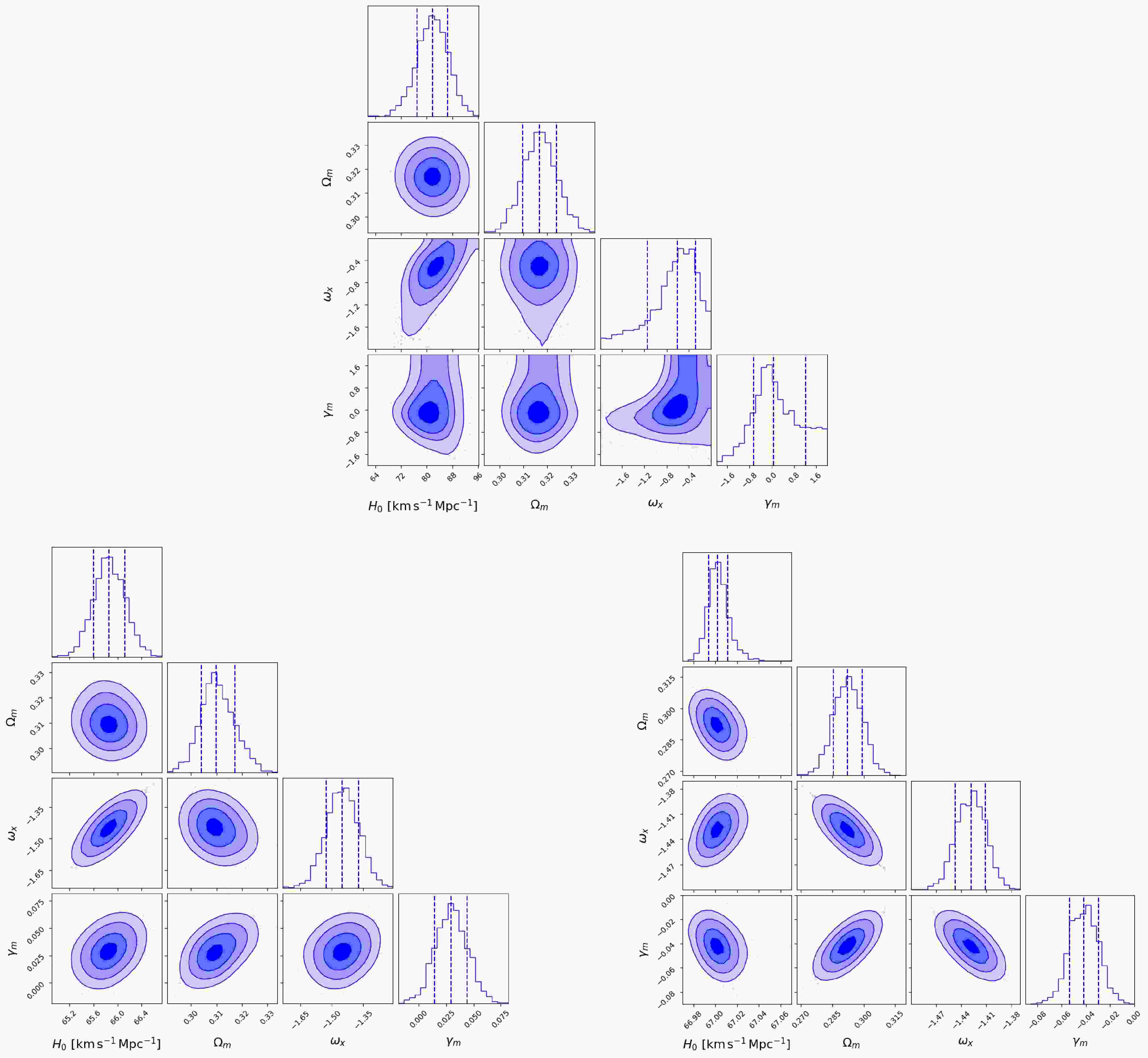
Here, $ \Omega_m = 8 \pi G \rho_{m0}/{(3 H_0^2)} $ is the current fractional energy density of matter. In our analysis, a Gaussian prior of $ \Omega_m = 0.317 \pm 0.007 $ is adopted, consistent with recent cosmological observations, to constrain its contribution. The remaining free parameters are $ H_0 $, $ \omega_x $, and $ \gamma_m $. Given the defined likelihood function, we employ the MCMC method to explore the posterior probability distributions of these three free parameters. We employ a screened set of 86 observational FRBs, together with two simulated datasets comprising 2,500 and 10,000 FRBs. The resulting posterior distributions are shown in Figure 1. When 86 observational FRB data constraints are applied, the best-fit values are determined as follows: the Hubble constant $ H_0 = 81.81^{+4.62}_{-4.88}\; {\rm{km}}\; {\rm{s}}^{-1}\; {\rm{Mpc}}^{-1} $, the dark energy equation of state parameter $ \omega_x = -0.61^{+0.33}_{-0.53} $, and the interaction parameter $ \gamma_m = 0.64^{+1.15}_{-0.71} $ at 68.3% confidence level.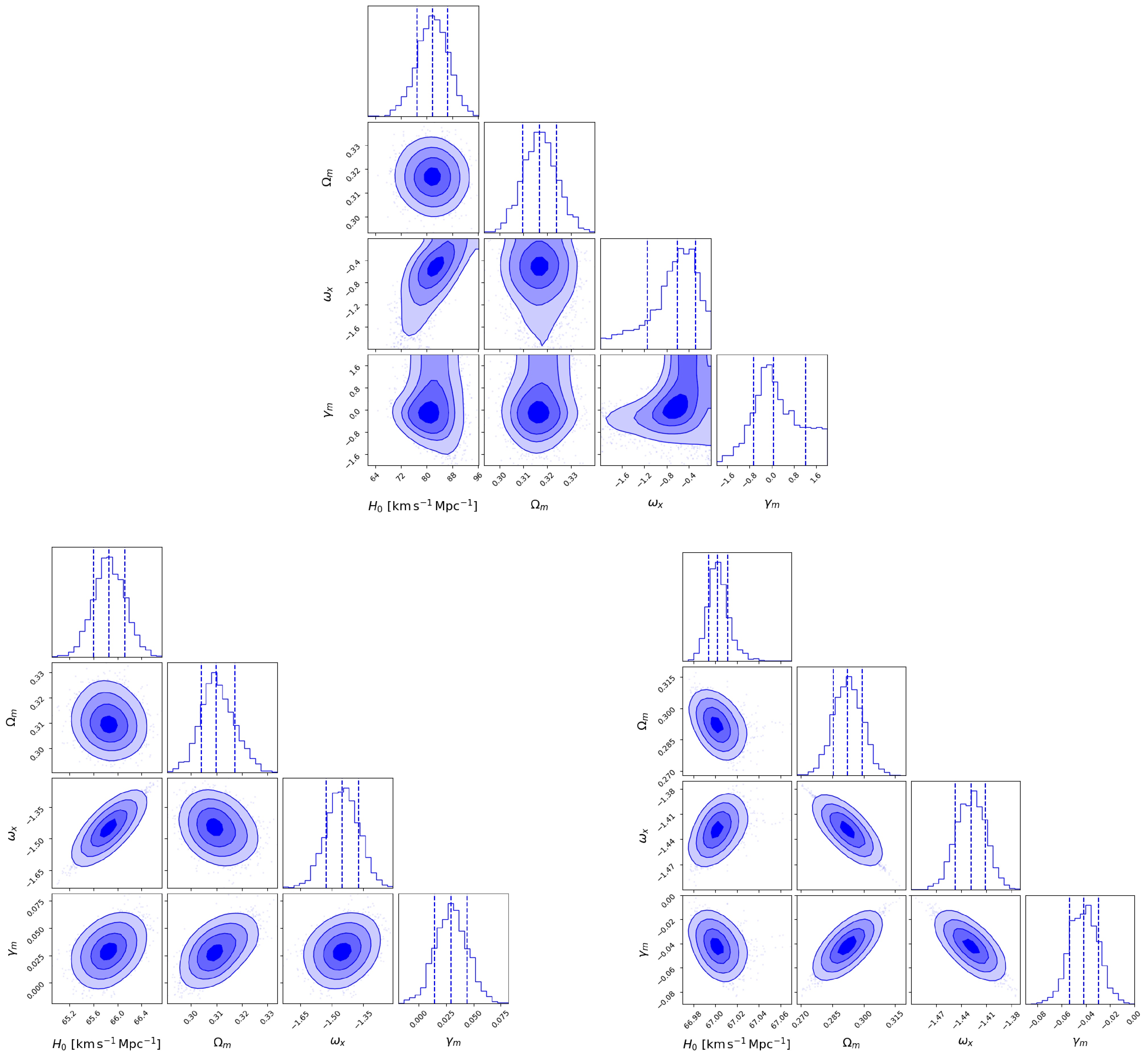

Figure 1.  (color online) Triangle plots showing constraints under the $ \gamma_m $IDE model. Top: constraints from real FRB observations. Bottom left: constraints from 2500 simulated FRBs. Bottom right: constraints from 10000 simulated FRBs. In each subfigure, the dashed lines from left to right correspond to the 16%, 50%, and 84% quantiles of the distribution. The diagonal shows marginalized posterior distributions for each parameter, while off-diagonal panels show joint distributions between parameter pairs.

Although the best-fit value of the interaction parameter $ \gamma_m $ between dark energy and dark matter is $ \gamma_m = 0.64^{+1.15}_{-0.71} $, indicating a mild preference for energy transfer from dark energy to dark matter and potential mitigation of the coincidence problem, the null-interaction case ($ \gamma_m = 0 $) still lies well within the 1σ confidence interval. This suggests that current data remain consistent with both interacting and non-interacting dark sector scenarios. The best-fit value of the dark energy equation-of-state parameter is slightly greater than −1, indicating a mild preference for quintessence-like behavior. Both the estimation and uncertainty of $ \omega_x $ in the $ \gamma_m $IDE model are consistent with the ΛCDM framework ($ \omega_x = -1 $), suggesting that the current data are not yet sufficient to distinguish the $ \gamma_m $IDE model from ΛCDM.

For subsequent model comparison in Section 5, we record the best-fit log-likelihood $ \ln {\cal{L}}_{{\rm{max}}} $ and the number of free parameters $ k=4 $ for BIC evaluation.

While current observational data provide useful constraints on the cosmological parameters, the relatively large uncertainties highlight the need for larger and more precise datasets. To further assess the constraining power of future FRB observations, we extend our analysis by incorporating two simulated FRB samples with significantly larger sizes. These mock datasets, consisting of 2,500 and 10,000 FRBs, are designed to mimic the statistical properties of real FRBs while significantly improving the data volume. Constraints based on the current sample of 86 localized FRBs provide a Hubble constant of $ H_0 = 81.81^{+4.62}_{-4.88}\; \;{\rm{km}}\;{\rm{s}}^{-1}\;{\rm{Mpc}}^{-1}, $ corresponding to an uncertainty of approximately $\pm 4.75 \;{\rm{km}}\;{\rm{s}}^{-1}\;{\rm{Mpc}}^{-1} $. The intermediate simulated sample of 2,500 FRBs reduces this uncertainty to $ \pm 0.26\; \;{\rm{km}}\;{\rm{s}}^{-1}\;{\rm{Mpc}}^{-1}, $ while the larger sample of 10,000 FRBs further reduces the uncertainty to $ \pm 0.01\; \;{\rm{km}}\;{\rm{s}}^{-1}\;{\rm{Mpc}}^{-1}. $ These results demonstrate the essential role of increased data volume in suppressing statistical fluctuations.

Similarly, the dark energy equation of state parameter $\omega_x $, currently constrained to $\omega_x = -0.61^{+0.33}_{-0.53} $ with an absolute uncertainty of approximately $\pm 0.43 $, sees its uncertainty reduced to $\pm 0.07 $ for the intermediate sample and further compressed to $\pm 0.02 $ for the large sample. As the sample size increases, the results exhibit clear convergence, indicating improved stability and reliability in the estimation of cosmological parameters.

For the coupling parameter $ \gamma_m $, the current broad constraint of $ 0.64^{+1.15}_{-0.71} $ ($ \pm 0.93 $) narrows significantly to $ \pm 0.015 $ with the intermediate sample, and further tightens to $ \pm 0.012 $ for the large sample, indicating improved parameter stability. The slight deviation of $ \omega_x $ from the standard cosmological value in the posterior results may be attributed to residual parameter degeneracies, which can shift the best-fit values even when statistical uncertainties are significantly reduced.

By performing a similar analysis as before using the interaction term $ Q_2 = 3\gamma_x H\rho_x $, which is proportional to the dark energy density, we obtain the Hubble parameter:

The free parameters in this model are $ H_0 $, $ \Omega_m $, $ \omega_x $, and $ \gamma_x $. Using the MCMC method, we obtained the best-fit values and posterior distributions of these parameters by fitting the model to different FRB datasets. The results are presented in Figure 2, which present the posterior distributions derived from three datasets: the real FRB sample, a mock sample of 2,500 simulated FRBs, and a mock sample of 10,000 simulated FRBs, providing constraints on the $ \gamma_x $ IDE model.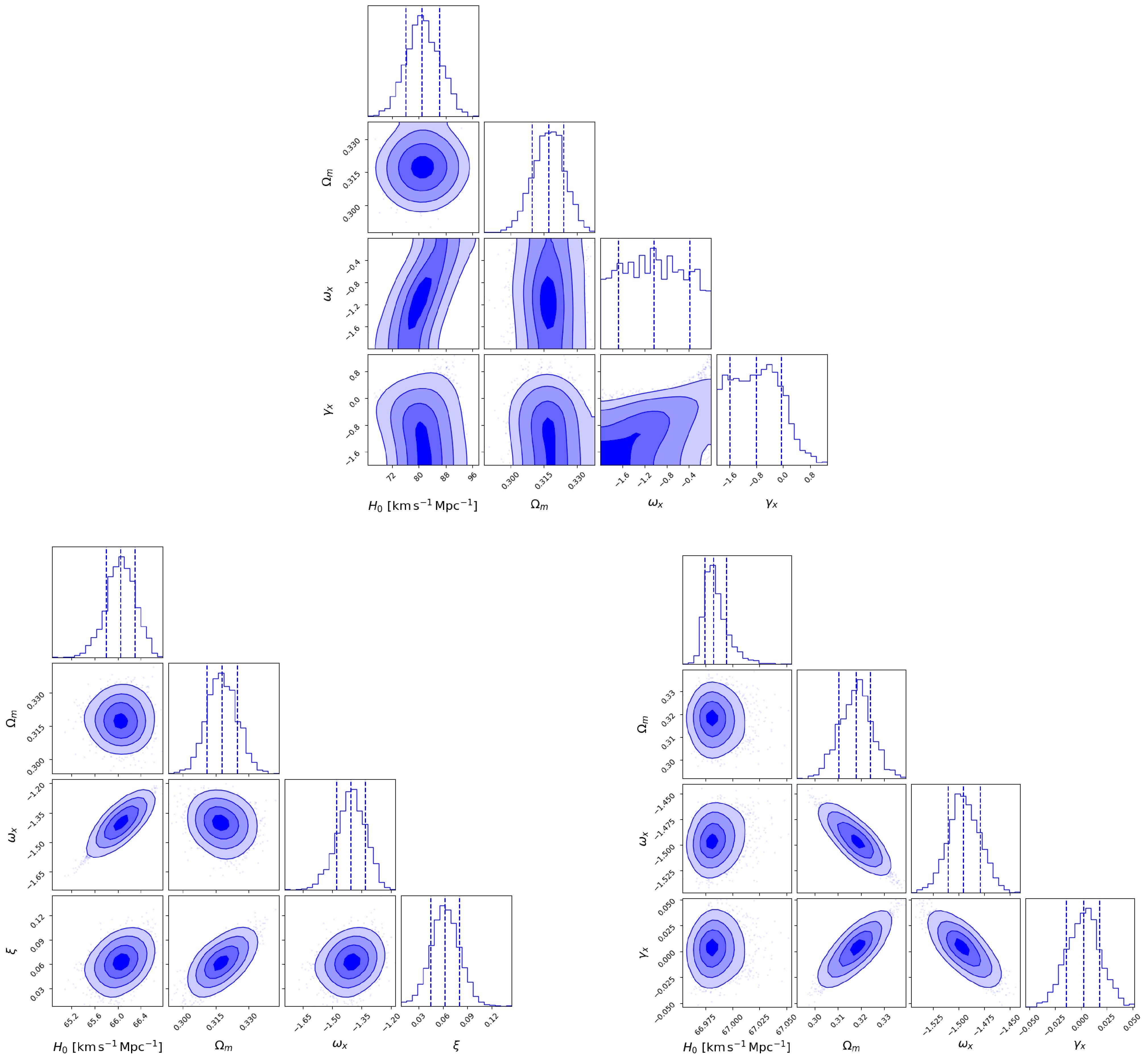

Figure 2.  (color online) The same as Figure 1, but for the $ \gamma_x $IDE model.

Using 86 localized FRBs, we obtain the following best-fit cosmological parameters: $ H_0 = 81.03^{+5.24}_{-4.88} \, \;{\rm{km}}\;{\rm{s}}^{-1} \;{\rm{Mpc}}^{-1} $ and $ \gamma_x = -0.80^{+0.75}_{-0.80} $ (68% confidence level). but that $ \omega_x $ is poorly constrained. Because the prior on $ \omega_x $ is uniform over the interval $ [-2, 0] $, only a median value of $ \thicksim -1.03 $ can be estimated. The best-fit value of $ \gamma_x $ indicates that the energy is transferred from dark matter to dark energy, and the coincidence problem is not alleviated.

As in previous cases, we record the best-fit log-likelihood $ \ln {\cal{L}}_{\rm{max}} $ and the number of free parameters $ k = 4 $ for BIC evaluation in Section 5.

While current constraints based on 86 localized FRBs yield a Hubble constant of $ H_0 = 81.03^{+5.24}_{-4.88}\; \;{\rm{km}}\;{\rm{s}}^{-1}\;{\rm{Mpc}}^{-1} $ with a relative error of 6.2%, the intermediate simulated sample significantly reduces this uncertainty to $ \pm 0.25\; \;{\rm{km}}\;{\rm{s}}^{-1}\;{\rm{Mpc}}^{-1} $. The large sample further compresses this uncertainty to $ \pm 0.01\; \;{\rm{km}}\;{\rm{s}}^{-1}\;{\rm{Mpc}}^{-1} $, underscoring the critical role of increased data volume in suppressing statistical fluctuations.

Similarly, the dark energy equation of state parameter $ \omega_x $, initially constrained to $ -1.03^{+0.65}_{-0.63} $ with an absolute uncertainty of $ \pm 0.64 $, sees its uncertainty reduced to $ \pm 0.07 $ for the intermediate sample and to $ \pm 0.016 $ for the large sample, demonstrating the potential of FRBs for precise cosmological parameter estimation.

For the coupling parameter $ \gamma_x $, the broad observational constraint of $ -0.80^{+0.75}_{-0.80} $ ($ \pm 0.78 $) narrows significantly to $ \pm 0.018 $ with the intermediate sample. This tightens further to $ \pm 0.016 $ for the large sample, indicating improved parameter stability but also highlighting the limited gains achievable through increased sample size alone due to parameter degeneracies. The slight posterior deviation of $ \omega_x $ from its standard cosmological value likely results from residual parameter degeneracies that can shift best-fit estimates despite reduced statistical uncertainties.

In the ξIDE model, the interaction term between dark matter and dark energy is expressed as $ Q_3 = \dfrac{-(1-\Omega_m)(\xi + 3\omega_x)}{1 - \Omega_m + \Omega_m(1+z)^\xi} H\rho_m. $ The corresponding dimensionless Hubble parameter is then given by

The free parameters are $ H_0 $, $ \Omega_m $, $ \omega_x $, and ξ. We employed the MCMC method to derive the best-fit values and posterior distributions of these parameters by fitting the model to various FRB datasets. The results are shown in Figure 3.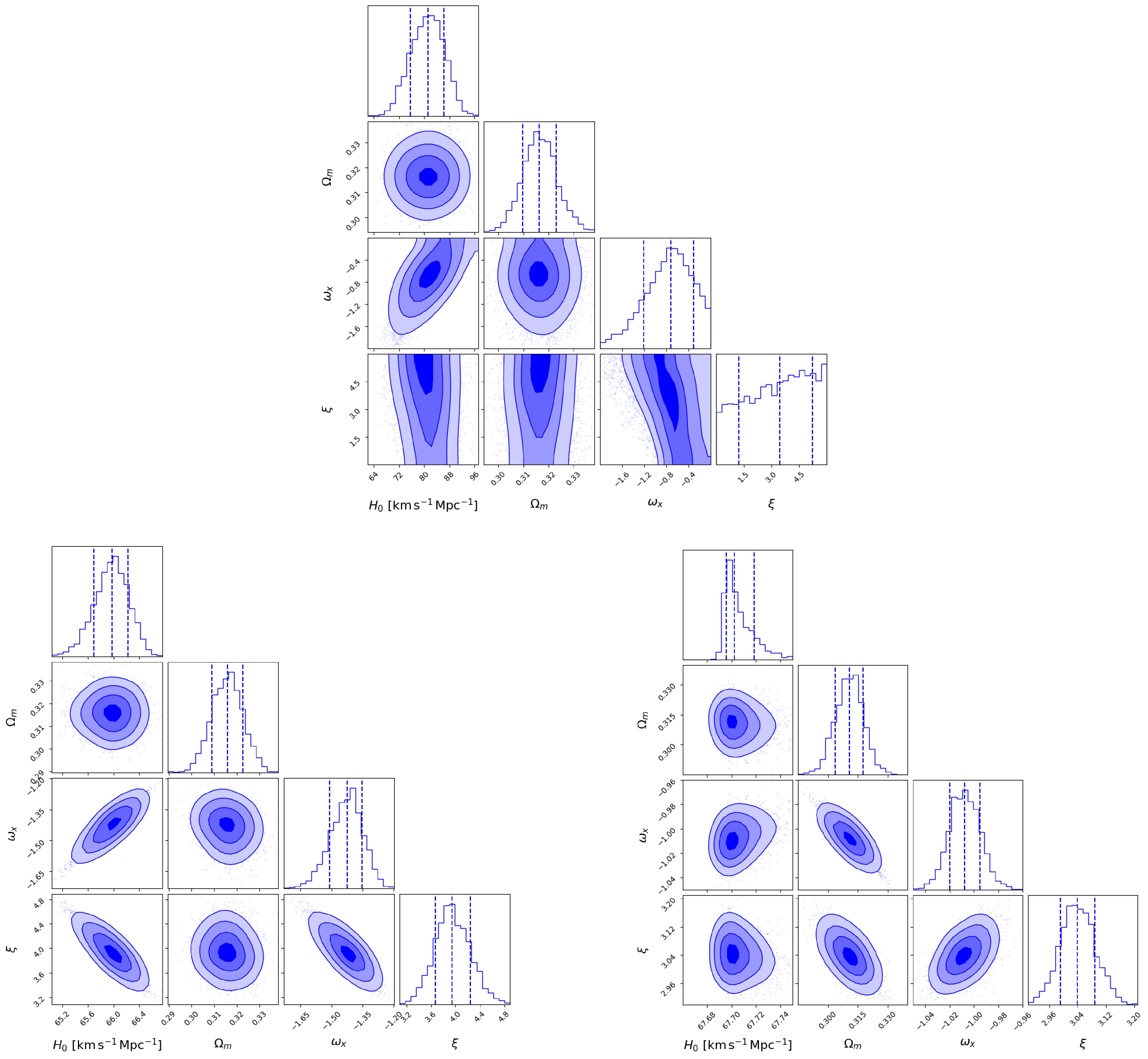

Figure 3.  (color online) The same as Figure 1, but for the ξIDE model.

For the real FRB sample, the best-fit values are $H_0 = 81.14^{+5.11}_{-5.60}\; {\rm{km}}\; {\rm{s}}^{-1}\; {\rm{Mpc}}^{-1} $ and $\omega_x = -0.72^{+0.41}_{-0.48} $ (68.3% confidence level). The parameter $\omega_x $ is poorly constrained, with the posterior distribution limited by the uniform prior over the interval $[-2, 0] $, allowing only a rough estimate of the median value at $\omega_x \sim 3.44 $. A strong degeneracy exists between $\omega_x $ and $\xi $, as both contribute to the effective coupling parameter $\gamma = -(\xi + 3\omega_x) $, which governs the energy transfer direction. A rough estimate of the central value yields $\gamma \sim -1.27 $, suggesting a mild energy transfer from dark matter to dark energy, and indicating that the coincidence problem is not alleviated.

As in previous sections, the best-fit log-likelihood $\ln {\cal{L}}_{\rm{max}} $ and the number of free parameters $k=4 $ are reported for model selection via the IC detailed in Section 5.

Using simulated datasets, the constraints tighten significantly as the sample size increases. For a mock sample of 2,500 FRBs, the parameter uncertainties shrink to $ H_0 = 65.98^{+0.25}_{-0.29}\ \;{\rm{km}}\;{\rm{s}}^{-1}\;{\rm{Mpc}}^{-1} $, $ \omega_x = -1.42^{+0.07}_{-0.09} $, and $ \xi = 3.94^{+0.30}_{-0.27} $. Expanding the sample to 10,000 FRBs further improves the precision, yielding $ H_0 = 67.70^{+0.01}_{-0.01}\ \;{\rm{km}}\;{\rm{s}}^{-1}\;{\rm{Mpc}}^{-1} $, $ \omega_x = -1.008^{+0.01}_{-0.01} $, and $ \xi = 3.04^{+0.05}_{-0.04} $. These results demonstrate a clear convergence toward the $\Lambda $CDM values, particularly $\xi = 3 $.

To systematically evaluate the performance of the three IDE models in fitting cosmological parameters, we employ IC for model comparison. These criteria balance model fit quality and complexity to identify the most statistically robust model. Specifically, we use three criteria: the Bayesian Information Criterion (BIC) [56], the Akaike Information Criterion (AIC) [57], and the Kullback Information Criterion (KIC) [58]. Previous studies have extensively investigated the application of BIC, AIC, and KIC in cosmological contexts [15, 59−61].

The BIC is given by

the AIC is defined as

and the KIC is defined as

Here, ${\cal{L}}_{\max} $ denotes the maximum likelihood, $k $ represents the number of parameters, and $N $ denotes the number of data points. For Gaussian errors, $\chi^2_{\min} = -2 \ln {\cal{L}}_{\max} $. We compute $\chi^2_{\min} $ and calculate the corresponding AIC, BIC, and KIC values, which are presented in Table 3.

IC	$ \gamma_m $IDE model	$ \gamma_x $IDE model	ξIDE model
$ \chi^2_{{\rm{min}}} $	1136.319	1136.347	1136.317
BIC	1154.137	1154.165	1154.134
AIC	1144.319	1144.347	1144.317
KIC	1148.319	1148.347	1148.317

Table 3.  IC values for the three models based on real data

The $ \gamma_m $IDE Model
	$ H_0 $ $ ({\rm{km}}\;{\rm{s}}^{-1}\;{\rm{Mpc}}^{-1}) $	$ \omega_x $	$ \gamma_m $
Observational FRB data	$ 81.81^{+4.62}_{-4.88}(1\sigma) $	$ -0.61^{+0.33}_{-0.53}(1\sigma) $	$ 0.64^{+1.15}_{-0.71}(1\sigma) $
Simulated FRB data(2500)	$ 65.856^{+0.258}_{-0.255}(1\sigma) $	$ -1.449^{+0.075}_{-0.073}(1\sigma) $	$ 0.0293^{+0.014}_{-0.015}(1\sigma) $
Simulated FRB data(10000)	$ 67.001^{+0.010}_{-0.008}(1\sigma) $	$ -1.428^{+0.018}_{-0.018}(1\sigma) $	$ -0.0416^{+0.012}_{-0.012}(1\sigma) $
The $ \gamma_x $IDE Model
	$ H_0 $ $ ({\rm{km}}\;{\rm{s}}^{-1}\;{\rm{Mpc}}^{-1}) $	$ \omega_x $	$ \gamma_x $
Observational FRB data	$ 81.03^{+5.24}_{-4.88}(1\sigma) $	$ -1.03^{+0.65}_{-0.63}(1\sigma) $	$ -0.80^{+0.75}_{-0.80}(1\sigma) $
Simulated FRB data(2500)	$ 66.055^{+0.247}_{-0.251}(1\sigma) $	$ -1.403^{+0.071}_{-0.075}(1\sigma) $	$ 0.062^{+0.018}_{-0.018}(1\sigma) $
Simulated FRB data(10000)	$ 66.982^{+0.013}_{-0.008}(1\sigma) $	$ -1.495^{+0.016}_{-0.015}(1\sigma) $	$ 0.002^{+0.015}_{-0.017}(1\sigma) $
The ξIDE Model
	$ H_0 $ $ ({\rm{km}}\;{\rm{s}}^{-1}\;{\rm{Mpc}}^{-1}) $	$ \omega_x $	ξ
Observational FRB data	$ 81.14^{+5.11}_{-5.60}(1\sigma) $	$ -0.72^{+0.41}_{-0.48}(1\sigma) $	$ 3.44^{+1.77}_{-2.19}(1\sigma) $
Simulated FRB data(2500)	$ 65.978^{+0.248}_{-0.287}(1\sigma) $	$ -1.424^{+0.072}_{-0.086}(1\sigma) $	$ 3.937^{+0.304}_{-0.271}(1\sigma) $
Simulated FRB data(10000)	$ 67.701^{+0.012}_{-0.006}(1\sigma) $	$ -1.008^{+0.013}_{-0.012}(1\sigma) $	$ 3.039^{+0.051}_{-0.047}(1\sigma) $

Table 2.  Best-fit values and 1σ uncertainties of the cosmological parameters in the three IDE models ($ \gamma_m $IDE, $ \gamma_x $IDE, and ξIDE) from FRB datasets: 86 real observations and two simulated samples (2,500 and 10,000 mock FRBs).

In the pairwise model comparison, the likelihood of model $ M_{\alpha} $ with information criterion value $ IC_{\alpha} $ is given by [62].

The difference $\Delta {\rm{IC}} = {\rm{IC}}_2 - {\rm{IC}}_1 $ quantifies the degree to which model $M_1 $ is favored over model $M_2 $ [63−65]. As an illustrative example, consider the comparison between the $ \gamma_m $IDE and $ \gamma_x $IDE models. Based on all three information criteria and using the real FRB sample, the probability that $ \gamma_m $IDE is the preferred model is $ P(M_1) \approx $50.4%, compared to $ P(M_2) \approx $49.6% for $ \gamma_x $IDE. This result indicates that $ \gamma_m $IDE yields slightly lower IC values than $ \gamma_x $IDE, though the difference is not statistically significant. A similar marginal difference is also observed between the $ \gamma_x $IDE and ξIDE models.

Finally, for the $\gamma_m $IDE and $\gamma_x $IDE models, the best-fit values of $\omega_x $ tend to be smaller than the fiducial value, likely due to parameter correlations. To verify this, we fix $H_0 = 67.4\; {\rm{km}}\; {\rm{s}}^{-1}\; {\rm{Mpc}}^{-1} $ and constrain the remaining three parameters ($\Omega_m $, $\gamma_m $, and $\omega_x $) with 2,500 simulated samples, following the same procedure as the previous four-parameter model. As shown in Figure 4, the best-fit values for the $\gamma_m $IDE model are $\omega_x = -1.01^{+0.012}_{-0.013} $; for the $\gamma_x $IDE model, they are $\omega_x = -1.011^{+0.012}_{-0.012} $. All parameters recover their fiducial values within the $1\sigma $ uncertainties.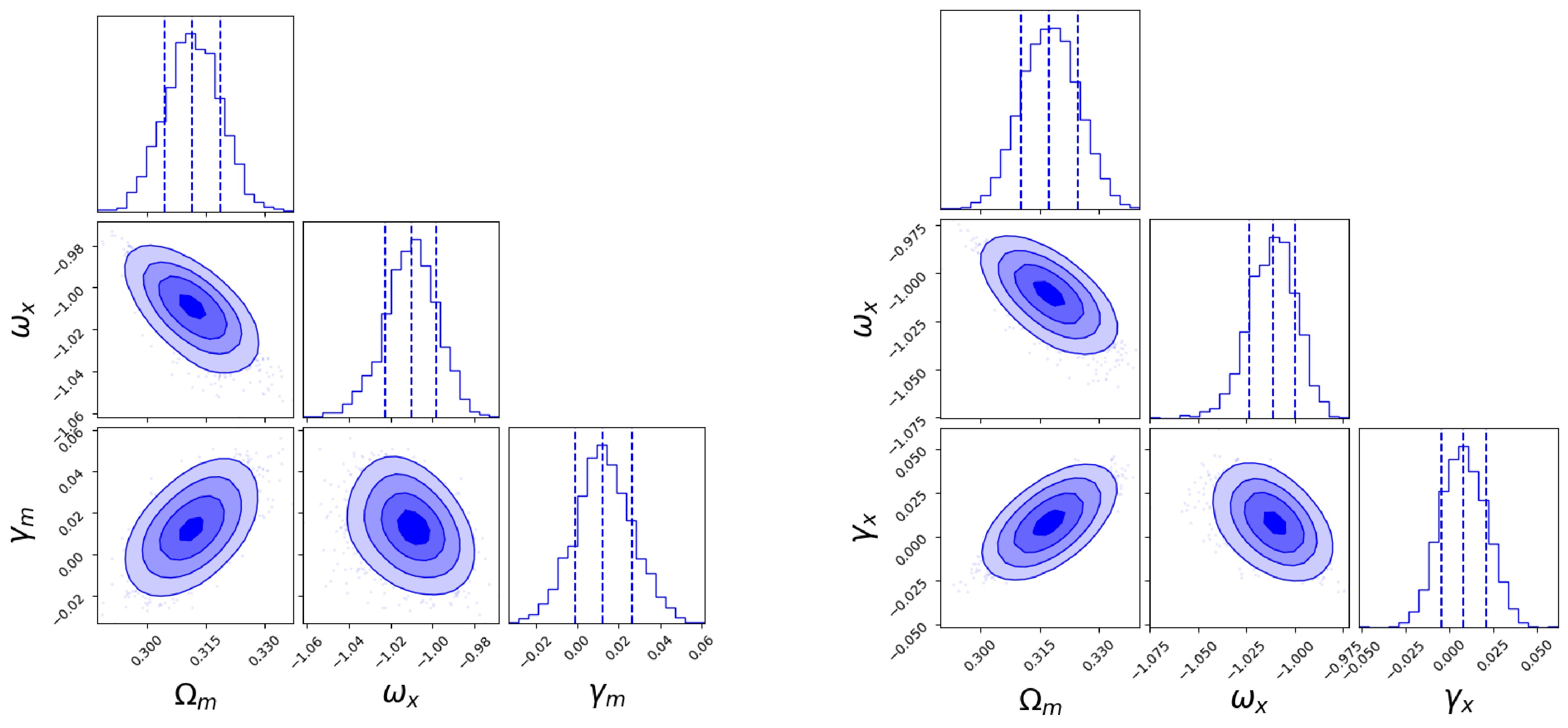

Figure 4.  (color online) Constraints on the remaining parameters of the $ \gamma_m $ and $ \gamma_x $ models using 2500 simulated FRBs, with $ H_0 $ fixed at 67.4 $ {\rm{km}}\; {\rm{s}}^{-1}\; {\rm{Mpc}}^{-1} $. The left panel shows the results for the $ \gamma_m $ model, while the right panel corresponds to the $ \gamma_x $ model.

In this paper, we explore the potential of FRBs to constrain cosmological parameters and investigate IDE models. We leverage the unique characteristics of FRBs, particularly their DMs, and redshifts, to perform a comprehensive analysis utilizing both observational and simulated FRB datasets.

We focus on three IDE models: the $\gamma_m $IDE, $\gamma_x $IDE, and $\xi $IDE models. Using Bayesian MCMC methods, we systematically evaluate the constraints on key cosmological parameters, namely the Hubble constant $H_0 $, the matter density parameter $\Omega_m $, the dark energy equation of state parameter $\omega_x $, and the interaction parameters $\gamma_m $, $\gamma_x $, and $\xi $.

First, we investigate three IDE models—$\gamma_m $IDE, $\gamma_x $IDE, and $\xi $IDE—using current localized FRB data alongside extended mock FRB samples. Based on observed FRB data, we find that the interaction term between dark energy and dark matter is consistent with zero within uncertainties, in agreement with previous studies constraining interaction parameters. In the $\gamma_m $IDE model, the interaction parameter $\gamma_m = 0 $ falls within the $1\sigma $ confidence interval, consistent with the standard $\Lambda $CDM model. However, the parameters $\omega_x $ in the $\gamma_x $IDE model and $\xi $ in the $\xi $IDE model are weakly constrained, resulting in posterior distributions that are nearly uniform across their prior ranges. This suggests that the current FRB dataset lacks sufficient constraining ability to confirm or exclude dark energy-dark matter interactions characterized by coupling terms proportional to matter density, dark energy density, or their ratio parameterized as a power-law of the scale factor.

With ongoing and upcoming radio telescopes, the number of localized FRBs is expected to increase significantly soon, and the redshift coverage will likely extend up to $ z \approx 3 $. To anticipate the constraining power of future data, we perform the same analysis using two mock datasets comprising 2,500 and 10,000 FRBs. We find that constraints on $H_0 $, $\omega_x $, and $\xi $ significantly improve with increasing sample size. However, the benefits for $\gamma_m $ and $\gamma_x $ exhibit diminishing returns, indicating a saturation in statistical gain. In the $\xi $IDE model, the parameters accurately recover their fiducial values $(H_0 = 67.4\; {\rm{km}}\; {\rm{s}}^{-1}\; {\rm{Mpc}}^{-1}, \omega_x = -1, \xi = 3) $ with increasing sample size, while in the $\gamma_m $IDE and $\gamma_x $IDE models, the parameter $\omega_x $ continues to deviate from its fiducial value, likely owing to residual parameter degeneracies.

Moreover, we provide three information criteria (AIC, BIC, and KIC) for each model in Table 3. The current observational data are insufficient to definitively discriminate among the three IDE models. Under the present FRB observations, the ξIDE model yields slightly lower IC values than the other two models, but the differences are not statistically significant.

Lastly, we investigate the impact of fixing $H_0 = 67.4\; {\rm{km}}\; {\rm{s}}^{-1}\; {\rm{Mpc}}^{-1} $ on parameter recovery using the $\gamma_m $IDE and $\gamma_x $IDE models with 2,500 mock FRBs. The resulting posterior distributions demonstrate that the parameters $\omega_x $ and $\gamma $ are more accurately recovered and consistent with the fiducial values, confirming the presence of residual degeneracies that can be mitigated by fixing certain parameters.

In conclusion, our results highlight the potential of FRBs in testing interacting dark energy scenarios. While current FRB data alone are insufficient to constrain dark energy–dark matter interactions, simulations suggest that future large and well-localized FRB samples could serve as robust cosmological probes, improving parameter estimation and enabling discrimination between interacting and non-interacting dark energy models.