


 Abstract
 HTML
HTML Reference
 Related
 PDF
PDF


-
Understanding the mass origin and the structure of baryons in the real world is a challenging problem. There is a conjecture dating back to the early days of the quark model that a baryon consists of a diquark (
$ qq $ pair) and another quark [1, 2]. The assumption of diquark reduces the number of levels in the baryon spectrum, which get closer to the experiment data than the three-body quark model. In this model, in order that the lowest-lying octet and decuplet baryons form a fully symmetric$ \mathbf{56} $ representation of the spin-flavor$ SU(6) $ , the diquark in lowest-lying baryons must be in a$ {}^3S_1 $ state, which corresponds to a spin-$ 1 $ boson. Later, some more realistic approaches derived from QCD also adopt the diquark picture [3−5], e.g., a Faddeev-type formulation which preserves the Lorentz and chiral symmetries. It is based on the observation that the gluon exchange between two quarks in the$ \bar{\mathbf{3}} $ representation of color$ SU(3) $ is known to be attractive, leading to a bound state. In this model the scalar diquarks play a significant role in the first baryon multiplet. Some recent progress can be found in, e.g., [6−9].In this work we consider the dynamics of quarks and diquarks in a two-dimensional toy model of QCD (
$ {\rm{QCD}}_2 $ ) with large-$ N_\mathrm{c} $ limit. For mesons consist of spinor quarks, this kind of model was first solved by 't Hooft [10], and was exhaustively studied in the subsequent works [11, 12, 14, 16–18, 46, 51]. For hadrons containing scalar quark and spinor antiquark. The two-dimensional scalar QCD (s$ {\rm{QCD}}_2 $ ) in the large-$ N_c $ limit has also been studied in the Feynman diagram approach [19], and in the Hamiltonian approach [20], both in the light-front quantization formalism. The interpretation of sQCD2 as a theory of diquark was also proposed in [21], where the mesonic bound states are thought as tetraquarks formed by a diquark-antidiquark pair. Recently, the equal-time quantization of sQCD2 in the Hamiltonian approach has been investigated in [22]. Following the same pattern, a baryon consists of a scalar quark and a spinor antiquark in two dimensions should be represented by the bound states of the spinor-scalar hybrid$ {\rm{QCD}}_2 $ . This kind of system was also studied in [23, 37] in the Feynman diagram approach and the light-front formalism.Our work focuses on the Hamiltonian approach and gives a thorough derivation of the light-front and equal-time quantization of both scalar and hybrid
$ {\rm{QCD}}_2 $ . We find that in s$ {\rm{QCD}}_2 $ , depending on the renormalizaion schemes of the mass, the renormalized mass in light-front may not coincide with that in equal-time. We derive the relation between these two renormalized masses. The novelty of our work is that the Hamiltonian approach is applied to the hybrid system. And we also carry out an exhaustive numerical analysis of the light-front and equal-time wave functions for scalar and hybrid bound state systems.The paper is organized as follows: In Sec. II, we review the derivation of the wave equation of the bound states in s
$ {\rm{QCD}}_2 $ , with an emphasis on the relation between the light-front and equal-time renormalizaion masses. In Sec. IIIA, we move on to the hybrid QCD2 and derive the wave equation for the scalar quark and spinor antiquark bound states. We exhibit the numerical results of the wave functions in Sec IV. We conclude in Sec. V. -
Understanding the hadron structure from QCD is the central mission of the contemporary hadron physics. Due to our limited knowledge about the color confinement mechanism, we are still unable to write down, let alone to solve, the bound-state equations (BSEs) pertaining to any hadron in terms of the relativistic quark and gluons degrees of freedom. There are some influential and powerful nonperturbative approaches, such as Dyson-Schwinger (DS)/Bethe-Salpeter (BS) equations [1−4], as well as light-front (LF) quantization [5−8], which, under some approximation, enable one to numerically solve the BSEs of hadron in Minkowski spacetime. Unfortunately, at practical level, these approaches heavily depend on some unsystematized truncation, whose prediction is thus subject to certain amount of model dependence.
The limit of infinite number of color, viz.,
$ 1/ N_\mathrm{c} $ expansion [9, 10], has proved to be a useful nonperturbative tool to help us to understand a number of some essential phenomena of QCD, such as Regge trajectory [10],$ U(1)_A $ problem [11, 12], and so on. Unfortunately, due to the enormous complexity of nonabelian gauge theory in four spacetime dimension, at present we still do not know how to write down the BSEs for a hadron even in the large$ N_c $ limit, let alone to deduce the nonperturbative features of a hadron in a quantitative manner.In 1974 't Hooft invented a solvable toy model of QCD, i.e., QCD in two spacetime dimensions meanwhile in the
$ N_\mathrm{c}\to\infty $ limit [13]. Thanks to the absence of transverse degree of freedom of the gauge field together with the planarity of Feynman diagrams, 't Hooft was able to write down the bound state equation of a meson in a closed form. The resulting discrete mesonic energy levels can be solved numerically, where the Regge trajectory becomes manifest. Soon it was also realized that 't Hooft model has also possesses some interesting properties like (naive) asymptotic freedom [14], nonvanishing quark condensate and “spontaneous” chiral symmetry breaking [15, 16]. Therefore, the 't Hooft model may be regarded as an instructive theoretical laboratory, which may help us to gain some insight into the nonperturbative aspects of QCD in the real world [14, 17−24].The BSE of 't Hooft model was originally derived with the aid of the diagrammatic technique based on the DS/BS equations, also within the context of light-front quantization. Therefore, the 't Hooft equation is valid only in the infinite momentum frame (IMF), viz., in which a meson moves with the speed of the light. It is worth noting that, an alternative approach to derive the 't Hooft equation is the operator approach based on bosonization of the light-front Hamiltonian, which has been extensively discussed in literature [25−31].
Poincaré invariance demands that the meson mass spectra must be identical in any inertial reference frame. One naturally wonders how the BSEs in 't Hooft model look like in the reference frame other than IMF. An important progress was made by Bars and Green in 1978 [32], who explicitly constructed a pair of coupled BSEs of mesons in
$ \text{QCD}_2 $ in the finite momentum frame (FMF), in which a meson moves with a finite momentum, including static case. The resulting BSEs pertaining to FMF, dubbed Bars-Green equation, is much more involved than the 't Hooft equation pertaining to IMF. It was also formally demonstrated that the Poincaré algebra does hold in the color-singlet subspace [32]. Later Poincaré invariance of meson spectrum has been explicitly verified by numerically solving Bars-Green in FMFs (static meson [20] and moving meson [23]).The advent of large momentum effective theory (LaMET) [33, 34] allows one to directly compute the partonic distributions of a hadron on the Euclidean lattice. A key element of LaMET is that, the quasi distributions, which are the matrix element of the equal-time, spacelike correlator sandwiched between a moving hadron state, under continuous Lorentz boost, will finally approach the light-cone parton distributions, which are the matrix element of the light-like correlator sandwiched between a hadron in IMF. 't Hooft model turns out to be a valuable theoretical laboratory to develop some intuition about the profiles of the quasi distributions. In the 't Hooft model, the light-cone distribution is simply linked with the 't Hooft wave function, and the quasi-distributions can be constructed in terms of the Bars-Green wave functions and Bogoliubov-chiral angle. It has been analytically and numerically verified that, a variety of quasi distributions in the 't Hooft model does converge to the light-cone distributions, as anticipated from LaMET [24, 35, 36].
Shortly after 't Hooft's original work, Shei and Tsao [37] in 1977 investigated the scalar
$ \text{QCD}_2 $ which instead contains bosonic quarks. With the aid of the diagrammatic approach in the context of LF quantization, Shei and Tsao also derived the BSE for a meson composed of a bosnic quark and a bosonic antiquark. The Shei-Tsao equation looks very similar to the 't Hooft equation. In 1978 Tomaras rederived the Shei-Tsao equation from the angle of Hamiltonian approach, and elaborated on some subtlety pertaining to quark mass renormalization [38]. Utilizing the Hamiltonian approach in the context of the equal-time quantization, Ji, Liu and Zahed have recently also derived the BSEs in scalar$ \text{QCD}_2 $ pertaining to FMF [39], and showed that these BSEs do approach the Shei-Tsao equation when boosted to the IMF.In the real world there is no bosonic quark. However, the notion of diquark turns out to be useful in baryon spectrum and structure, at least on the phenomenological ground
1 . In 2008 Grinstein, Jora and Polosa investigated the mesonic mass spectra in scalar$ \text{QCD}_2 $ [49], who argued that, a bosonic quark may mimick a diquark to some extent, therefore the meson in scalar$ \text{QCD}_2 $ may be related to the tetraquark state in the real world, which is conjectured to consist of a compact diquark and anti-diquark. It is expected that the study of the “tetraquark” spectrum in scalar$ \text{QCD}_2 $ [49] may shed some light on the tetraquark spectrum in the realistic QCD4 [49].It is difficult to investigate the BSE for a baryon in the original 't Hooft model, since a baryon would become infinitely heavy in the
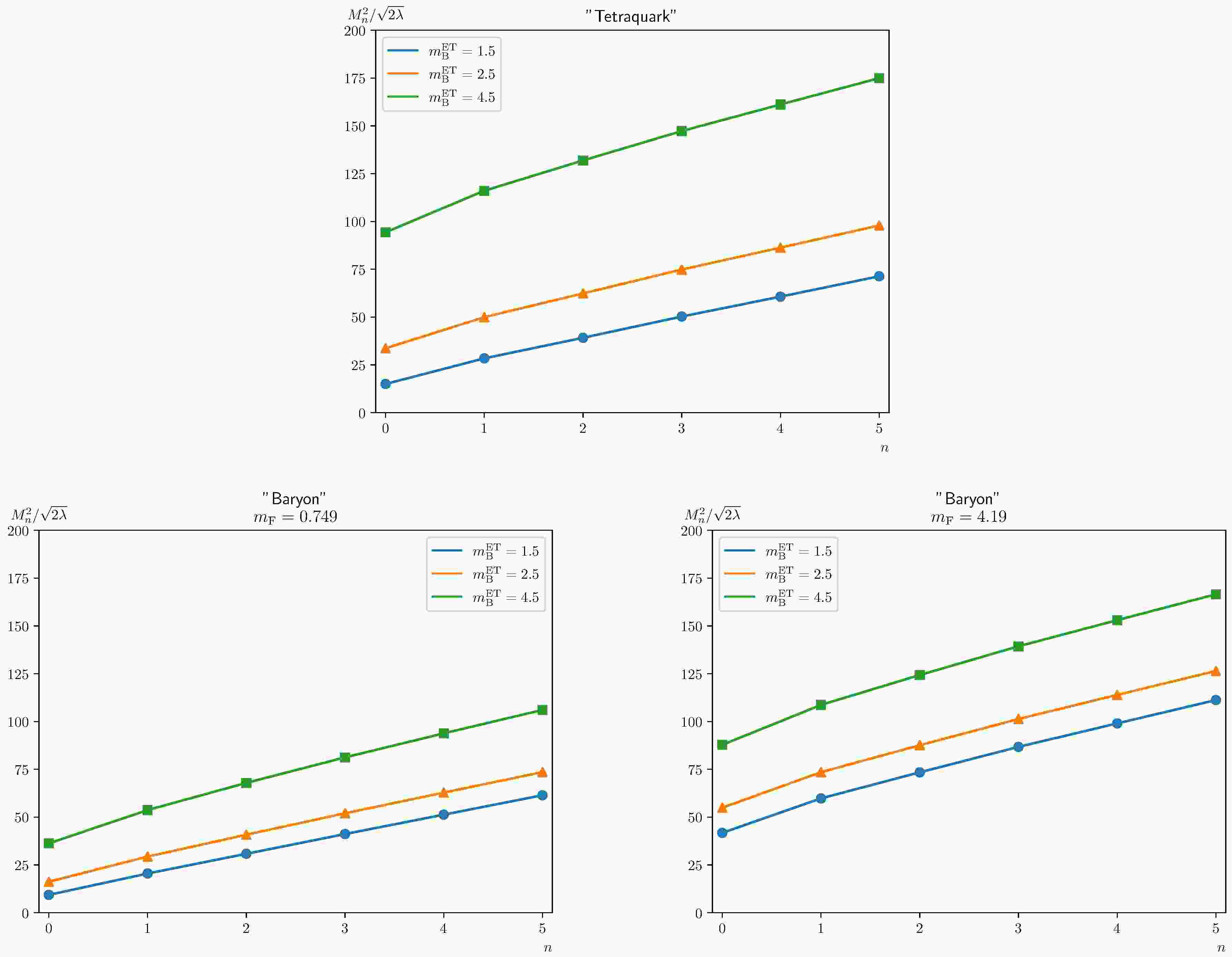
$ N_c\to \infty $ limit. Nevertheless, once accepting the notion of the diquark, one may mimick a “baryon” by a bound state formed by a bosonic quark and fermionic antiquark in the extended 't Hooft model. The BSE for such a “baryon” state in IMF was first obtained with the aid of diagrammatic technique by Aoki [50].It is the primary goal to derive the BSEs for a “baryon” state in the extended 't Hooft model in FMF, which constitute the counterparts of the Bars-Green equations of mesons in the original 't Hooft model. We also conduct a comprehensive numerical study of the “baryon” spectrum and the bound-state wave functions of the lowest-lying baryon. It is especially interesting to visualize how the wave functions in the FMF evolve to the light-cone wave functions when increasing the momentum of the “baryon”.
We use the Hamiltonian approach in equal-time quantization with a “fermionization” procedure to derive the BSEs of “baryon” in FMF. For the sake of completeness, we also revisit the derivation of BSE of “baryon” in the IMF from the angle of the Hamiltonian approach in LF quantization. Since the “baryon” contains a bosonic quark, the BSEs of which are intimated connected with those of “tetraquark” composed entirely of bosonic quark and antiquark. Therefore, to facilitate a coherent reading, we feel it beneficial to give a self-contained treatment of both types of exotic hadrons. Therefore we decide to revisit the derivations of the BSEs of the “tetraquark in IMF and FMF using Hamiltonian approach, which were originally done in [38, 39]. Some subtle issue about the quark mass renormalization in LF and equal-time quantization in scalar
$ \text{QCD}_2 $ is highlighted. Moreover, it is worth pointing out that the diagrammatic derivation of the BSEs of a “tetraquark” in FMF is much difficult than its counterpart in IMF, since the seagull vertex does not vanish even after taking the axial gauge. A novel outcome of this work is to successfully reproduce the BSEs of “tetraquark” from the angle of the diagrammatic DS/BS approaches.The rest of the paper is organized as follows. In Sec. II, we define the extended 't Hooft model and set up some notations. In Sec. III, we revisit the derivation of BSEs of an “tetraquark” in both IMF and FMF, with some emphasis on the relation between the renormalized quark mass in LF and equal-time quantization. Sec. IV constitutes the main body of this work, where we derive the BSEs of a “baryon” in both IMF and FMF. The BSEs in FMF are obtained for the first time. In Sec V we present the numerical results of the mass spectra of “tetraquark” and “baryon”. In particular, we show the numerical profiles of the bound-state wave functions of the lowest-lying states, with different hadron velocities. We summarize in Sec. VI. We devote Appendix A to a diagrammatic derivation of the corresponding BSEs of “tetraquark” in FMF. In Appendix B, we present a detailed discussion on the connection between two renormalized quark masses introduced in LF quantization and equal-time quantization for the “tetraquark” case.
-
Understanding the hadron structure from QCD is the central mission of the contemporary hadron physics. Due to our limited knowledge about the color confinement mechanism, we are still unable to write down, let alone to solve, the bound-state equations (BSEs) pertaining to any hadron in terms of the relativistic quark and gluons degrees of freedom. There are some influential and powerful nonperturbative approaches, such as Dyson-Schwinger (DS)/Bethe-Salpeter (BS) equations [1−4], as well as light-front (LF) quantization [5−8], which, under some approximation, enable one to numerically solve the BSEs of hadron in Minkowski spacetime. Unfortunately, at practical level, these approaches heavily depend on some unsystematized truncation, whose prediction is thus subject to certain amount of model dependence.
The limit of infinite number of color, viz.,
$ 1/ N_\mathrm{c} $ expansion [9, 10], has proved to be a useful nonperturbative tool to help us to understand a number of some essential phenomena of QCD, such as Regge trajectory [10],$ U(1)_A $ problem [11, 12], and so on. Unfortunately, due to the enormous complexity of nonabelian gauge theory in four spacetime dimension, at present we still do not know how to write down the BSEs for a hadron even in the large$ N_c $ limit, let alone to deduce the nonperturbative features of a hadron in a quantitative manner.In 1974 't Hooft invented a solvable toy model of QCD, i.e., QCD in two spacetime dimensions meanwhile in the
$ N_\mathrm{c}\to\infty $ limit [13]. Thanks to the absence of transverse degree of freedom of the gauge field together with the planarity of Feynman diagrams, 't Hooft was able to write down the bound state equation of a meson in a closed form. The resulting discrete mesonic energy levels can be solved numerically, where the Regge trajectory becomes manifest. Soon it was also realized that 't Hooft model has also possesses some interesting properties like (naive) asymptotic freedom [14], nonvanishing quark condensate and ''spontaneous'' chiral symmetry breaking [15, 16]. Therefore, the 't Hooft model may be regarded as an instructive theoretical laboratory, which may help us to gain some insight into the nonperturbative aspects of QCD in the real world [14, 17−24].The BSE of 't Hooft model was originally derived with the aid of the diagrammatic technique based on the DS/BS equations, also within the context of light-front quantization. Therefore, the 't Hooft equation is valid only in the infinite momentum frame (IMF), viz., in which a meson moves with the speed of the light. It is worth noting that, an alternative approach to derive the 't Hooft equation is the operator approach based on bosonization of the light-front Hamiltonian, which has been extensively discussed in literature [25−31].
Poincaré invariance demands that the meson mass spectra must be identical in any inertial reference frame. One naturally wonders how the BSEs in 't Hooft model look like in the reference frame other than IMF. An important progress was made by Bars and Green in 1978 [32], who explicitly constructed a pair of coupled BSEs of mesons in
$ \text{QCD}_2 $ in the finite momentum frame (FMF), in which a meson moves with a finite momentum, including static case. The resulting BSEs pertaining to FMF, dubbed Bars-Green equation, is much more involved than the 't Hooft equation pertaining to IMF. It was also formally demonstrated that the Poincaré algebra does hold in the color-singlet subspace [32]. Later Poincaré invariance of meson spectrum has been explicitly verified by numerically solving Bars-Green in FMFs (static meson [20] and moving meson [23]).The advent of large momentum effective theory (LaMET) [33, 34] allows one to directly compute the partonic distributions of a hadron on the Euclidean lattice. A key element of LaMET is that, the quasi distributions, which are the matrix element of the equal-time, spacelike correlator sandwiched between a moving hadron state, under continuous Lorentz boost, will finally approach the light-cone parton distributions, which are the matrix element of the light-like correlator sandwiched between a hadron in IMF. 't Hooft model turns out to be a valuable theoretical laboratory to develop some intuition about the profiles of the quasi distributions. In the 't Hooft model, the light-cone distribution is simply linked with the 't Hooft wave function, and the quasi-distributions can be constructed in terms of the Bars-Green wave functions and Bogoliubov-chiral angle. It has been analytically and numerically verified that, a variety of quasi distributions in the 't Hooft model does converge to the light-cone distributions, as anticipated from LaMET [24, 35, 36].
Shortly after 't Hooft's original work, Shei and Tsao [37] in 1977 investigated the scalar
$ \text{QCD}_2 $ which instead contains bosonic quarks. With the aid of the diagrammatic approach in the context of LF quantization, Shei and Tsao also derived the BSE for a meson composed of a bosnic quark and a bosonic antiquark. The Shei-Tsao equation looks very similar to the 't Hooft equation. In 1978 Tomaras rederived the Shei-Tsao equation from the angle of Hamiltonian approach, and elaborated on some subtlety pertaining to quark mass renormalization [38]. Utilizing the Hamiltonian approach in the context of the equal-time quantization, Ji, Liu and Zahed have recently also derived the BSEs in scalar$ \text{QCD}_2 $ pertaining to FMF [39], and showed that these BSEs do approach the Shei-Tsao equation when boosted to the IMF.In the real world there is no bosonic quark. However, the notion of diquark turns out to be useful in baryon spectrum and structure, at least on the phenomenological ground
1 . In 2008 Grinstein, Jora and Polosa investigated the mesonic mass spectra in scalar$ \text{QCD}_2 $ [49], who argued that, a bosonic quark may mimick a diquark to some extent, therefore the meson in scalar$ \text{QCD}_2 $ may be related to the tetraquark state in the real world, which is conjectured to consist of a compact diquark and anti-diquark. It is expected that the study of the ''tetraquark'' spectrum in scalar$ \text{QCD}_2 $ [49] may shed some light on the tetraquark spectrum in the realistic QCD4 [49].It is difficult to investigate the BSE for a baryon in the original 't Hooft model, since a baryon would become infinitely heavy in the
$ N_c\to \infty $ limit. Nevertheless, once accepting the notion of the diquark, one may mimick a ''baryon'' by a bound state formed by a bosonic quark and fermionic antiquark in the extended 't Hooft model. The BSE for such a ''baryon'' state in IMF was first obtained with the aid of diagrammatic technique by Aoki [50].It is the primary goal to derive the BSEs for a ''baryon'' state in the extended 't Hooft model in FMF, which constitute the counterparts of the Bars-Green equations of mesons in the original 't Hooft model. We also conduct a comprehensive numerical study of the ''baryon'' spectrum and the bound-state wave functions of the lowest-lying baryon. It is especially interesting to visualize how the wave functions in the FMF evolve to the light-cone wave functions when increasing the momentum of the ''baryon''.
We use the Hamiltonian approach in equal-time quantization with a ''fermionization'' procedure to derive the BSEs of ''baryon'' in FMF. For the sake of completeness, we also revisit the derivation of BSE of ''baryon'' in the IMF from the angle of the Hamiltonian approach in LF quantization. Since the ''baryon'' contains a bosonic quark, the BSEs of which are intimated connected with those of ''tetraquark'' composed entirely of bosonic quark and antiquark. Therefore, to facilitate a coherent reading, we feel it beneficial to give a self-contained treatment of both types of exotic hadrons. Therefore we decide to revisit the derivations of the BSEs of the ''tetraquark in IMF and FMF using Hamiltonian approach, which were originally done in [38, 39]. Some subtle issue about the quark mass renormalization in LF and equal-time quantization in scalar
$ \text{QCD}_2 $ is highlighted. Moreover, it is worth pointing out that the diagrammatic derivation of the BSEs of a ''tetraquark'' in FMF is much difficult than its counterpart in IMF, since the seagull vertex does not vanish even after taking the axial gauge. A novel outcome of this work is to successfully reproduce the BSEs of ''tetraquark'' from the angle of the diagrammatic DS/BS approaches.The rest of the paper is organized as follows. In Sec. II, we define the extended 't Hooft model and set up some notations. In Sec. III, we revisit the derivation of BSEs of an ''tetraquark'' in both IMF and FMF, with some emphasis on the relation between the renormalized quark mass in LF and equal-time quantization. Sec. IV constitutes the main body of this work, where we derive the BSEs of a ''baryon'' in both IMF and FMF. The BSEs in FMF are obtained for the first time. In Sec. V we present the numerical results of the mass spectra of ''tetraquark'' and ''baryon''. In particular, we show the numerical profiles of the bound-state wave functions of the lowest-lying states, with different hadron velocities. We summarize in Sec. VI. We devote Appendix A to a diagrammatic derivation of the corresponding BSEs of ''tetraquark'' in FMF. In Appendix B, we present a detailed discussion on the connection between two renormalized quark masses introduced in LF quantization and equal-time quantization for the ''tetraquark'' case.
-
The extended 't Hooft model contains both bosonic and fermionic quarks and gluons. For simplicity, we only consider a single species of bosonic quark and fermionic quark. The corresponding hybrid
$ \text{QCD}_2 $ Lagrangian is dictated by the$ SU \left(N_{\rm{c}}\right) $ gauge invariance:$ {\cal{L}}_{h \text{QCD}_2} = -\frac{1}{4}\left(F_{\mu\nu}^a\right)^2 + \bar{\psi} (i \not D-m_F) \psi + \left(D^{\mu}\phi\right)^{\dagger}D_{\mu}\phi - m_B^2\phi^{\dagger}\phi, $
(1) where ψ and ϕ denote the Dirac and complex scalar fields,
$ m_F $ and$ m_B $ refer to the masses of the bosonic and fermionic quarks, and$ A_{\mu}^a $ represents the gluon field with color index$ a = 1,2,\cdots, N_\mathrm{c}^2-1 $ .$ D_{\mu} = \partial_{\mu} - i g_{s} A_{\mu}^{a}T^a $ signifies the color covariant derivative, and$ F_{\mu\nu}^{a}\equiv\partial_{\mu}A_{\nu}^{a}-\partial_{\nu}A_{\mu}^{a}+g_{s}f^{abc}A_{\mu}^{b}A_{\nu}^{c} $ represents the gluonic field strength tensor.The generators of
$ SU \left(N_{\rm{c}}\right) $ group in the fundamental representation obey the following relation:$ \mathrm{tr}(T^{a}T^{b}) = \frac{\delta^{ab}}{2}, $
(2a) $ \sum\limits_{a}T_{ij}^{a}T_{kl}^{a} = \frac{1}{2}\left(\delta_{il}\delta_{jk}-\frac{1}{N_c}\delta_{ij}\delta_{kl}\right). $
(2b) The Lorentz two-vector is defined as
$ x^{\mu} = \left(x^{0},x^{z}\right) $ , with the superscript$ 0 $ and z representing the time and spatial indices. The Dirac γ-matrices in two space-time dimensions are represented by$ \gamma^{0} = \sigma_{1},\qquad \gamma^{z} = -i\sigma_{2},\qquad \gamma^{5}\equiv\gamma^{0}\gamma^{z} = \sigma_{3}, $
(3) where
$ \sigma^i $ ($ i = 1,2,3 $ ) signifies the Pauli matrices.In LF quantization it is also convenient to adopt the light-cone coordinates, which are defined through
$ x^\pm = x_\mp = \left(x^0 \pm x^z\right)/\sqrt{2} $ , with the light-front time denoted by$ x^+ $ .Throughout this work, we are interested in the large-
$ N_\mathrm{c} $ limit:$ N_\mathrm{c} \rightarrow \infty,\qquad\qquad \lambda \equiv \frac{ g_\mathrm{s}^2 N_\mathrm{c}}{4\pi}\text{ fixed}, $
(4) with λ referring to the 't Hooft coupling constant. We are also tacitly working in the so-called weak coupling limit, where
$ m_F, m_B\gg g \sim 1/\sqrt{N_c} $ [15]. -
The extended 't Hooft model contains both bosonic and fermionic quarks and gluons. For simplicity, we only consider a single species of bosonic quark and fermionic quark. The corresponding hybrid
$ \text{QCD}_2 $ Lagrangian is dictated by the$ S U \left(N_{\rm{c}}\right) $ gauge invariance:$ {\cal{L}}_{h \text{QCD}_2} = -\frac{1}{4}\left(F_{\mu\nu}^a\right)^2 + \bar{\psi} ({\rm i} \not D-m_F) \psi + \left(D^{\mu}\phi\right)^{\dagger}D_{\mu}\phi - m_B^2\phi^{\dagger}\phi, $
(1) where ψ and ϕ denote the Dirac and complex scalar fields,
$ m_F $ and$ m_B $ refer to the masses of the fermionic and bosonic quarks, and$ A_{\mu}^a $ represents the gluon field with color index$ a = 1,2,\cdots, N_\mathrm{c}^2-1 $ .$ D_{\mu} = \partial_{\mu} - {\rm i} g_{s} A_{\mu}^{a}T^a $ signifies the color covariant derivative, and$ F_{\mu\nu}^{a}\equiv\partial_{\mu}A_{\nu}^{a}-\partial_{\nu}A_{\mu}^{a}+g_{s}f^{abc}A_{\mu}^{b}A_{\nu}^{c} $ represents the gluonic field strength tensor.The generators of
$ S U \left(N_{\rm{c}}\right) $ group in the fundamental representation obey the following relation:$ \mathrm{tr}(T^{a}T^{b}) = \frac{\delta^{ab}}{2}, $
(2a) $ \sum\limits_{a}T_{ij}^{a}T_{kl}^{a} = \frac{1}{2}\left(\delta_{il}\delta_{jk}-\frac{1}{N_c}\delta_{ij}\delta_{kl}\right). $
(2b) The Lorentz two-vector is defined as
$ x^{\mu} = \left(x^{0},x^{z}\right) $ , with the superscript$ 0 $ and z representing the time and spatial indices. The Dirac γ-matrices in two space-time dimensions are represented by$ \gamma^{0} = \sigma_{1},\qquad \gamma^{z} = -{\rm i}\sigma_{2},\qquad \gamma^{5}\equiv\gamma^{0}\gamma^{z} = \sigma_{3}, $
(3) where
$ \sigma^i $ ($ i = 1,2,3 $ ) signifies the Pauli matrices.In LF quantization it is also convenient to adopt the light-cone coordinates, which are defined through
$ x^\pm = x_\mp = \left(x^0 \pm x^z\right)/\sqrt{2} $ , with the light-front time denoted by$ x^+ $ .Throughout this work, we are interested in the large-
$ N_\mathrm{c} $ limit:$ N_\mathrm{c} \rightarrow \infty,\qquad \lambda \equiv \frac{ g_\mathrm{s}^2 N_\mathrm{c}}{4\pi}\text{ fixed}, $
(4) with λ referring to the 't Hooft coupling constant. We are also tacitly working in the so-called weak coupling limit, where
$ m_F, m_B\gg g \sim 1/\sqrt{N_c} $ [15]. -
In this section we only focus on the bosonic quark. For simplicity, we consider only one single flavor of quark. The corresponding scalar
$ {\rm QCD}_2 $ lagrangian is entirely dictated by the$ SU(N_c) $ gauge invariance:$ \mathcal{L}_{\mathrm{sQCD}_2}= -\frac{1}{4}\left(F_{\mu\nu}^a\right)^2 + \left(D^{\mu}\phi\right)^{\dagger}D_{\mu}\phi - m^2\phi^{\dagger}\phi, $

(1) where ϕ denotes the complex scalar field, m represents the current quark mass, and
$ A_{\mu}^a $ represents the gluon field with color index$ a=1,2,\cdots, N_c^2-1 $ .$ F_{\mu\nu}^{a}\equiv\partial_{\mu}A_{\nu}^{a}- \partial_{\nu}A_{\mu}^{a}+g_{s}f^{abc}A_{\mu}^{b}A_{\nu}^{c} $ is the gluonic field strength tensor, and$ D_{\mu} = \partial_{\mu} - i g_{s} A_{\mu}^{a}T^a $ signifies the color covariant derivative. The generators of$ S U\left(N_c\right) $ group in the fundamental representation obey the following relation:$ \mathrm{tr}(T^{a}T^{b}) = \frac{\delta^{ab}}{2}, \tag{2a}$

$ \sum\limits_{a}T_{ij}^{a}T_{kl}^{a} = \frac{1}{2}\left(\delta_{il}\delta_{jk}-\frac{1}{N_c}\delta_{ij}\delta_{kl}\right). \tag{2b} $

The Lorentz two-vector is defined as
$ x^{\mu}=\left(x^{0},x^{z}\right) $ , with the superscript$ 0 $ and z representing the time and spatial indices. The Dirac γ-matrices in two space-time dimensions are represented by$ \gamma^{0}=\sigma_{1},\qquad \gamma^{z}=-i\sigma_{2},\qquad \gamma^{5}\equiv\gamma^{0}\gamma^{z}=\sigma_{3}, $

(3) where
$ \sigma^i $ ($ i=1,2,3 $ ) signifies the Pauli matrices.Throughout this work, we are interested in the so-called large-
$ N_\mathrm{c} $ limit:$ N_\mathrm{c} \rightarrow \infty,\qquad\qquad \lambda \equiv \frac{ g_\mathrm{s}^2 N_\mathrm{c}}{4\pi}\text{ fixed}, $

(4) with λ referring to the 't Hooft coupling constant.
-
In this section we first revisit the derivation of BSE of a “tetraquark” in IMF, then revisit the derivation of the BSEs of a “tetraquark” in FMF. Some special attention is paid to the quark mass renormalization in both LF and equal-time quantization.
-
In this section we first revisit the derivation of BSE of a ''tetraquark'' in IMF, then revisit the derivation of the BSEs of a ''tetraquark'' in FMF. Some special attention is paid to the quark mass renormalization in both LF and equal-time quantization.
-
The bound-state equation in the spinor QCD
$ _{2} $ was originally derived by 't Hooft in 1974, with the aid of diagrammatic Dyson-Schwinger/Bethe-Salpeter approach in the context of light-front quantization. Shortly after, the light-front bound-state equation in scalar QCD$ _{2} $ was also derived by Shei et al. in 1977 [19]. An equivalent approach to derive the bound-state equation is the Hamiltonian operator method, which has been widely applied in the context of the spinor QCD$ _{2} $ [25−31]. In 1978 Tomaras rederived the light-front bound-state equation in scalar QCD$ _{2} $ , verifying Shei et al.'s equations and elaborate on some subtlety about the quark mass renormalization [20] Loosely speaking, since a scalar bosonic quark may mimick a diquark to some extent, Grinstein et al. [21] in 2008 investigated the mesonic mass spectra in scalar QCD$ _{2} $ , which may shed some light on the tetraquark spectrum in the realistic QCD$ _4 $ .In this subsection, we revisit the operator approach derivation of the bound-state equations in scalar QCD
$ _{2} $ within the light-front quantization framework, paying special attention to the mass renormalization issue. -
We start with rederivation of the BSE of ''tetraquark'' in the IMF using the operator approach [38]. For this purpose, it is most convenient to quantize the scalar
$ \text{QCD}_2 $ in equal LF time. -
We start with rederivation of the BSE of “tetraquark” in the IMF using the operator approach [38]. For this purpose, it is most convenient to quantize the scalar
$ \text{QCD}_2 $ in equal LF time. -
Similar to spinor QCD
$ _{2} $ , the scalar QCD$ _{2} $ becomes significantly simplified once imposing the light-cone gauge$ A^{+a}=0 $ :$ \mathcal{L}_{\mathrm{sQCD}_2} = \frac{1}{2}\left(\partial_-A^{-a}\right)^2 + \left(\partial_-\phi^\dagger\right) D_+\phi + \left(D_+\phi\right)^\dagger \partial_-\phi - m^2\phi^\dagger\phi. $

(5) It is convenient to adopt the light-cone coordinates, which are defined through
$ x^\pm = x_\mp = \left(x^0 \pm x^z\right)/\sqrt{2} $ , with light-front time denoted by$ x^+ $ . The canonic conjugate momenta are given by$ \pi \equiv \dfrac{\partial\mathcal{L}}{\partial\left(\partial_+\phi^\dagger\right)} = \partial_-\phi,\:\pi^\dagger = \partial_-\phi^\dagger $ . One immediately arrives at the corresponding light-front Hamiltonian:$ \begin{aligned}[b] H_ \text{LF} =&\int dx^-\Bigg(-\frac{1}{2}\left(\partial_-A^{-a}\right)^{2}+ig_{s}A^{-a}\\&\times\left(\pi^{\dagger}T^{a}\phi-\phi^{\dagger}T^{a}\pi\right)+m^{2}\phi^{\dagger}\phi\Bigg). \end{aligned} $

(6) Since the light-front time derivative of the gluon field is absent in the lagrangian (5), the gluonic field
$ A^{-a} $ is no longer a dynamical variable. In fact, it is subject to a the following constraint:$ \begin{array}{*{20}{l}} \partial_-^2A^{-a} = g_\mathrm{s} J^a, \end{array} $

(7) where
$ J^{a}\equiv i\left(\phi^{\dagger}T^{a}\pi-\pi^{\dagger}T^{a}\phi\right) $ .Solving
$ A^{-a} $ in term of$ J^a $ in (7), and substituting back into (6), the light-front Hamiltonian then reduces to$ H_ \text{LF} =\int dx^-\left(m^{2}\phi^{\dagger}\phi-\frac{g_{s}^{2}}{2}J^{a}\frac{1}{\partial_-^{2}}J^{a}\right). $

(8) The light-front Hamiltonian actually becomes nonlocal. To see this, note that the rigorous meaning of
$ 1/\partial_-^2 J^a $ in (8) is$ \frac{1}{\partial_-^2} J^a\left(x^-\right) = \int dy^- G^{(2)}_\rho\left(x^–y^-\right) J^a\left(y^-\right), $

(9) where
$ G^{(2)} $ represents the Green function$ \partial_-^{2}G^{\left(2\right)}\left(x^-\right)=\delta\left(x^-\right). $

(10) The actual solution of the Green function turns out to be
$ G_\rho^{(2)}\left(x^–y^-\right) = -\int_{-\infty}^{+\infty} \frac{dk^+}{2\pi}\Theta\left(\left|k^+\right|-\rho\right) \frac{e^{ik^+\left(x^–y^-\right)}}{\left(k^+\right)^2}. $

(11) To make the Green function mathematically well-defined, we introduce an infrared cutoff ρ to regularize the severe IR divergence. This parameter may also be viewed as an artificial gauge parameter. Needless to say, this fictitious parameter must disappear in the final expressions for any physical quantities.
-
We express the scalar
$ \text{QCD}_2 $ lagrangian in terms of light-cone coordinates. Similar to the original 't Hooft model, a great simplification can be achieved by imposing the light-cone gauge$ A^{+a} = 0 $ 2 :$ {\cal{L}}_{\mathrm{sQCD}_2} = \frac{1}{2}\left(\partial_-A^{-a}\right)^2 + \left(\partial_-\phi^\dagger\right) D_+\phi + \left(D_+\phi\right)^\dagger \partial_-\phi - m^2\phi^\dagger\phi. $
(5) The canonical conjugate momenta of bosonic quark fields are given by
$ \pi \equiv \dfrac{\partial{\cal{L}}}{\partial\left(\partial_+\phi^\dagger\right)} = \partial_-\phi $ and$ \pi^\dagger = \partial_-\phi^\dagger $ . After Legendre transformation, one arrives at the following LF Hamiltonian:$ \begin{aligned}[b]H_ \text{LF} =\;& \int dx^-\Bigg(-\frac{1}{2}\left(\partial_-A^{-a}\right)^{2}+ig_{s}A^{-a}\left(\pi^{\dagger}T^{a}\phi-\phi^{\dagger}T^{a}\pi\right)\\&+m^{2}\phi^{\dagger}\phi\Bigg).\end{aligned} $
(6) Due to the absence of the light-front time derivative of the gluon field in (5),
$ A^{-a} $ is no longer a dynamical variable, which is subject to the following constraint:$ \partial_-^2A^{-a} = g_\mathrm{s} J^a, $
(7) with
$ J^{a}\equiv i\left(\phi^{\dagger}T^{a}\pi-\pi^{\dagger}T^{a}\phi\right) $ .Solving
$ A^{-a} $ in term of$ J^a $ in (7), and substituting back into (6), one then reduces the LF Hamiltonian to$ H_ \text{LF} = \int dx^-\left(m^{2}\phi^{\dagger}\phi-\frac{g_{s}^{2}}{2}J^{a}\frac{1}{\partial_-^{2}}J^{a}\right). $
(8) The LF Hamiltonian now becomes nonlocal. Note that the rigorous meaning of
$ 1/\partial_-^2 J^a $ in (8) is$ \frac{1}{\partial_-^2} J^a\left(x^-\right) = \int dy^- G^{(2)}_\rho\left(x^-y^-\right) J^a\left(y^-\right), $
(9) where
$ G^{(2)} $ represents the Green function$ \partial_-^{2} G^{\left(2\right)}\left(x^-\right) = \delta\left(x^-\right). $
(10) The actual solution of the Green function turns out to be
$ G_\rho^{(2)}\left(x^-y^-\right) = -\int_{-\infty}^{+\infty} \frac{dk^+}{2\pi}\Theta\left(\left|k^+\right|-\rho\right) \frac{e^{ik^+\left(x^-y^-\right)}}{\left(k^+\right)^2}. $
(11) To render
$ G^{(2)} $ mathematically well-defined, we have introduced an infrared cutoff ρ to regularize the severe IR divergence pertaining to$ k^+\to 0 $ . This parameter may also be viewed as an artificial gauge parameter. Needless to say, this fictitious parameter must disappear in the final expressions for any physical entities. -
We express the scalar
$ \text{QCD}_2 $ lagrangian in terms of light-cone coordinates. Similar to the original 't Hooft model, a great simplification can be achieved by imposing the light-cone gauge$ A^{+a} = 0 $ 2 :$ {\cal{L}}_{\mathrm{sQCD}_2} = \frac{1}{2}\left(\partial_-A^{-a}\right)^2 + \left(\partial_-\phi^\dagger\right) D_+\phi + \left(D_+\phi\right)^\dagger \partial_-\phi - m^2\phi^\dagger\phi. $
(5) The canonical conjugate momenta of bosonic quark fields are given by
$ \pi \equiv \dfrac{\partial{\cal{L}}}{\partial\left(\partial_+\phi^\dagger\right)} = \partial_-\phi $ and$ \pi^\dagger = \partial_-\phi^\dagger $ . After Legendre transformation, one arrives at the following LF Hamiltonian:$ \begin{aligned}[b]H_ \text{LF} =\;& \int {\rm d}x^-\Bigg(-\frac{1}{2}\left(\partial_-A^{-a}\right)^{2}+ {\rm i} g_{s}A^{-a}\left(\pi^{\dagger}T^{a}\phi-\phi^{\dagger}T^{a}\pi\right)\\&+m^{2}\phi^{\dagger}\phi\Bigg).\end{aligned} $
(6) Due to the absence of the light-front time derivative of the gluon field in (5),
$ A^{-a} $ is no longer a dynamical variable, which is subject to the following constraint:$ \partial_-^2A^{-a} = g_\mathrm{s} J^a, $
(7) with
$ J^{a}\equiv {\rm i}\left(\phi^{\dagger}T^{a}\pi-\pi^{\dagger}T^{a}\phi\right) $ .Solving
$ A^{-a} $ in term of$ J^a $ in (7), and substituting back into (6), one then reduces the LF Hamiltonian to$ H_ \text{LF} = \int {\rm d}x^-\left(m^{2}\phi^{\dagger}\phi-\frac{g_{s}^{2}}{2}J^{a}\frac{1}{\partial_-^{2}}J^{a}\right). $
(8) The LF Hamiltonian now becomes nonlocal. Note that the rigorous meaning of
$ 1/\partial_-^2 J^a $ in (8) is$ \frac{1}{\partial_-^2} J^a\left(x^-\right) = \int {\rm d}y^- G^{(2)}_\rho\left(x^-y^-\right) J^a\left(y^-\right), $
(9) where
$ G^{(2)} $ represents the Green function$ \partial_-^{2} G^{\left(2\right)}\left(x^-\right) = \delta\left(x^-\right). $
(10) The actual solution of the Green function turns out to be
$ G_\rho^{(2)}\left(x^-y^-\right) = -\int_{-\infty}^{+\infty} \frac{{\rm d}k^+}{2\pi}\Theta\left(\left|k^+\right|-\rho\right) \frac{{\rm e}^{{\rm i}k^+\left(x^-y^-\right)}}{\left(k^+\right)^2}. $
(11) To render
$ G^{(2)} $ mathematically well-defined, we have introduced an infrared cutoff ρ to regularize the severe IR divergence pertaining to$ k^+\to 0 $ . This parameter may also be viewed as an artificial gauge parameter. Needless to say, this fictitious parameter must disappear in the final expressions for any physical entities. -
We impose the canonical quantization for the scalar
$ \text{QCD}_2 $ in (8) in equal LF time. It is convenient to Fourier-expand the ϕ and π fields in terms of the quark and antiquark's annihilation and creation operators:$ \phi^i\left(x^-\right) = \int_0^\infty\frac{{\rm d}k^+}{2\pi}\frac{1}{\sqrt{2k^+}} \left[a^{i}\left(k^+\right){\rm e}^{{\rm -i}k^+x^-}+c^{i\dagger}\left(k^+\right){\rm e}^{{\rm i}k^+x^-}\right], $
(12a) $\begin{aligned}[b] \pi^{j\dagger}\left(x^-\right) =\;& {\rm i}\int_0^\infty\frac{{\rm d}k^+}{2\pi} \sqrt{\frac{k^+}{2}}\Big[a^{j\dagger}\left(k^+\right){\rm e}^{{\rm i}k^+x^-}\\&-c^{j}\left(k^+\right){\rm e}^{{\rm -i}k^+x^-}\Big].\end{aligned} $
(12b) where
$ i,j = 1,\cdots, N_\mathrm{c} $ are color indices. The annihilation and creation operators are assumed to obey the standard commutation relations:$ \left[a^i\left(k^+\right), a^{j\dagger}\left(p^+\right)\right] = \left[c^i\left(k^+\right), c^{j\dagger}\left(p^+\right)\right] = \left(2\pi\right)\delta\left(k^+-p^+\right)\delta^{ij}. $
(13) A useful trick to diagonalize the Hamiltonian is the bosonization technique [25−31]. One first introduces the following four compound color-singlet operators:
$\begin{aligned}[b]& W\left(k^+,p^+\right) \equiv\frac{1}{\sqrt{ N_\mathrm{c}}}\sum\limits_{i}c^{i}\left(k^+\right)a^{i}\left(p^+\right), \\& W^{\dagger}\left(k^+,p^+\right) \equiv\frac{1}{\sqrt{ N_\mathrm{c}}}\sum\limits_{i}a^{i\dagger}\left(p^+\right)c^{i\dagger}\left(k^+\right) ,\end{aligned} $
(14a) $\begin{aligned}[b]& A\left(k^+,p^+\right) \equiv\sum\limits_{i}a^{i\dagger}\left(k^+\right)a^{i}\left(p^+\right), \\& C\left(k^+,p^+\right) \equiv\sum\limits_{i}c^{i\dagger}\left(k^+\right)c^{i}\left(p^+\right).\end{aligned} $
(14b) It is straightforward to find the commutation relations among these four compound operators:
$\begin{aligned}[b]& \left[W\left(k_{1}^+,p_{1}^+\right),W^{\dagger}\left(k_{2}^+,p_{2}^+\right)\right] \\=\;& \left(2\pi\right)^{2}\delta\left(k_{1}^+-k_{2}^+\right)\delta\left(p_{1}^+-p_{2}^+\right)+{\cal{O}}\left(\frac{1}{ N_\mathrm{c}}\right),\end{aligned} $
(15a) $ \left[W\left(k_{1}^+,p_{1}^+\right),A\left(k_{2}^+,p_{2}^+\right)\right] = 2\pi\delta\left(p_{1}^+-k_2^+\right) W\left(k_1^+,p_{2}^+\right), $
(15b) $ \left[W\left(k_{1}^+,p_{1}^+\right),C\left(k_{2}^+,p_{2}^+\right)\right] = 2\pi\delta\left(k_1^+-k_2^+\right) W\left(p_{2}^+,p_{1}^+\right), $
(15c) $\begin{aligned}[b]& \left[A\left(k_{1}^+,p_{1}^+\right),A\left(k_{2}^+,p_{2}^+\right)\right] \\=\;& 2\pi\delta\left(p_{1}^+-k_2^+\right)A\left(k_1^+,p_{2}^+\right) - 2\pi\delta\left(p_{2}^+-k_1^+\right) A\left(k_2^+,p_{1}^+\right),\end{aligned} $
(15d) $\begin{aligned}[b]& \left[C\left(k_{1}^+,p_{1}^+\right),C\left(k_{2}^+,p_{2}^+\right)\right]\\ =\;& 2\pi\delta\left(p_{1}^+-k_2^+\right)C\left(k_1^+,p_{2}^+\right) - 2\pi\delta\left(p_{2}^+-k_1^+\right) C\left(k_2^+,p_{1}^+\right),\end{aligned} $
(15e) $ \left[A\left(k_{1}^+,p_{1}^+\right),C\left(k_{2}^+,p_{2}^+\right)\right] = 0. $
(15f) Substituting (12) into the LF Hamiltonian in (8), and express everything in terms of the compound operator basis as specified in (14), we can break the light-front Hamiltonian into three pieces:
$ H_{\rm{LF}} = H_{\rm{LF;0}}+\colon H_{\rm{LF;2}}\colon+\colon H_{\rm{LF;4}}\colon+{\cal{O}}\left(\frac{1}{\sqrt{ N_\mathrm{c}}}\right), $
(16) whose explicit expressions read
$ H_{\rm{LF;0}} = N_c \int \frac{{\rm d}x^-}{2\pi}\Bigg(\int_0^\infty\frac{{m^{2}}{{\rm d}k^+}}{2k^+}-{\pi\lambda}\int_0^\infty\frac{{\rm d}k_{3}^+}{2\pi}\int_0^\infty \frac{{\rm d}k_{4}^+}{2\pi}\frac{\left(k_{3}^+-k_{4}^+\right)^2}{\left(k_{3}^++k_{4}^+\right)^{2}{k_3^+k_4^+}} \Theta\left(|k_{3}^++k_{4}^+|-\rho\right)\Bigg), $
(17a) $ \begin{aligned}[b] :H_{\rm{LF;2}}: =\;& {m^{2}}\int_0^\infty\frac{{\rm d}k^+}{2\pi{2k^+}} \left[A\left(k^+,k^+\right)+C\left(k^+,k^+\right)\right] +\int_0^\infty\frac{{\rm d}k_{1}^+}{2\pi}\int_{-\infty}^\infty\frac{{\rm d}k_{2}^+}{2\pi}\frac{2\pi\lambda}{k_{1}^+ |k_{2}^+|}\left(\frac{k_{1}^++k_{2}^+}{k_{2}^+-k_{1}^+}\right)^{2} \\ &\times \Theta(|k_{2}^+-k_{1}^+|-\rho)[ A\left(k_{1}^+,k_{1}^+\right)+ C\left(k_{1}^+,k_{1}^+\right)] , \end{aligned} $
(17b) $ \begin{aligned}[b] :H_{\rm{LF;4}}: =\;& -{\pi^{3}\lambda} \int_0^\infty\frac{{\rm d}k_{1}^+}{2\pi\sqrt{k_{1}^+}}\int_0^\infty\frac{{\rm d}k_{2}^+}{2\pi\sqrt{k_{2}^+}} \int_0^\infty\frac{{\rm d}k_{3}^+}{2\pi\sqrt{k_{3}^+}}\int_0^\infty\frac{{\rm d}k_{4}^+}{2\pi\sqrt{k_{4}^+}} \frac{1}{\left(k_{3}^+-k_{4}^+\right)^{2}} \\& \times\Theta\left(|k_{3}^+-k_{4}^+|-\rho\right) \left(k_{1}^++k_{2}^+\right)\left(k_{4}^++k_{3}^+\right)\times\big[W^{\dagger}\left(k_{4}^+,k_{1}^+\right) W\left(k_{3}^+,k_{2}^+\right) \delta\left(k_{1}^+-k_{2}^++k_{4}^+-k_{3}^+\right) \\ & + W^{\dagger}\left(k_{2}^+,k_{3}^+\right)W\left(k_{1}^+,k_{4}^+\right) \delta\left(k_{2}^+-k_{1}^++k_{3}^+-k_{4}^+\right)\big], \end{aligned} $
(17c) with
$ :\;\:: $ denoting the normal ordering.$ H_{\rm{LF;0}} $ denotes the LF energy of the vacuum, which appears to be severely IR divergent.The confinement characteristics of QCD indicates that all the physical excitation must be the color singlets. In the color-singlet subspace of states, the compound operators A and C are not independent operators, which, at lowest order in
$ 1/ N_\mathrm{c} $ , actually can be expressed as the convolution between the color-singlet quark-antiquark pair creation/annihilation operators W and$ W^{\dagger} $ in (14a):$ A(k^+,p^+) \rightarrow \int_0^\infty\frac{{\rm d}q^+}{2\pi} W^\dagger(q^+,k^+)W(q^+,p^+), $
(18a) $ C(k^+,p^+) \rightarrow \int_0^\infty\frac{{\rm d}q^+}{2\pi} W^\dagger(k^+,q^+)W(p^+,q^+). $
(18b) Plugging (18) into (17b) and (17c), and relabelling the momenta in
$ W^{(\dagger)}\left(k^+,p^+\right) $ by$ p^+ = xP^+ $ ,$ k^+ = (1-x)P^+ $ , we can rewrite the :$ H_{\rm{LF;2}}: $ and :$ H_{\rm{LF;4}} $ : pieces at the lowest order in$ 1/ N_\mathrm{c} $ as$ \begin{aligned}[b] :H_{\rm{LF;2}}: =\;& \int_{0}^{\infty} \frac{{\rm d}P^+\,P^+}{(2\pi)^2}\int_0^1 {\rm d}x W^{\dagger}\left(\left(1-x\right)P^+,xP^+\right)W\left(\left(1-x\right)P^+,xP^+\right) \Bigg[\frac{m^{2}}{2xP^+}+\frac{m^{2}}{2(1-x)P^+} \\&+\frac{\lambda}{8xP^+}\int_{-\infty}^\infty\frac{{\rm d}y}{|y|} \frac{\left(x+y\right)^2}{\left(y-x\right)^2}\Theta\left(|(y-x)P^+|-\rho\right)+\frac{\lambda}{8(1-x)P^+}\int_{-\infty}^\infty\frac{{\rm d}y}{|1-y|} \frac{\left(2-x-y\right)^2}{\left(y-x\right)^2}\Theta\left(|(y-x)P^+|-\rho\right)\Bigg], \end{aligned}$
(19a) $ \begin{aligned}[b] :H_{\rm{LF;4}}: =\;& -\frac{\lambda}{2\left(2\pi\right)^{2}} \int_0^1 {\rm d}x\int_0^1 {\rm d}y\int_{0}^{\infty} \frac{{\rm d}P^+\left(P^+\right)^{2}}{2\pi} W^{\dagger}\left(\left(1-x\right)P^+,xP^+\right)W\left(\left(1-y\right)P^+,yP^+\right) \\ &\times\frac{1}{\sqrt{xP^+}}\frac{1}{\sqrt{yP^+}}\frac{1}{\sqrt{(1-y)P^+}}\frac{1}{\sqrt{(1-x)P^+}}\frac{1}{[(x-y)P^+]^{2}}\Theta\left(|(x-y)P^+|-\rho\right)\left[\left(1-x\right)P^++\left(1-y\right)P^+\right]\left(yP^++xP^+\right). \end{aligned} $
(19b) -
The task is to quantize the Hamiltonian (8) in equal light-front time. We Fourier-expand the ϕ and π fields in terms of the quark/antiquark's annihilation and creation operators:
$ \begin{aligned}[b] \phi^i\left(x^-\right) =& \int_0^\infty\frac{dk^+}{2\pi}\frac{1}{\sqrt{2k^+}} \Bigg[a^{i}\left(k^+\right)e^{-ik^+x^-}\\&+c^{i\dagger}\left(k^+\right)e^{ik^+x^-}\Bigg], \end{aligned} \tag{12a}$

$ \begin{aligned}[b] \pi^{j\dagger}\left(x^-\right) =& i\int_0^\infty\frac{dk^+}{2\pi} \sqrt{\frac{k^+}{2}}\Bigg[a^{j\dagger}\left(k^+\right)e^{ik^+x^-}\\&-c^{j}\left(k^+\right)e^{-ik^+x^-}\Bigg]. \end{aligned}\tag{12b} $

where
$ i,j=1,\cdots,N_c $ are color indices. The annihilation and creation operators are assumed to obey the standard commutation relations:$ \begin{array}{*{20}{l}} \left[a^i\left(k^+\right), a^{j\dagger}\left(p^+\right)\right] = \left[c^i\left(k^+\right), c^{j\dagger}\left(p^+\right)\right] = \left(2\pi\right)\delta\left(k^+-p^+\right)\delta^{ij}. \end{array} $

(13) A useful trick to diagonalize the Hamiltonian is the bosonization technique [25−31]. One first introduces the following four compound color-singlet operators:
$ \begin{aligned}[b] W\left(k^+,p^+\right) &\equiv\frac{1}{\sqrt{ N_\mathrm{c}}}\sum\limits_{i}c^{i}\left(k^+\right)a^{i}\left(p^+\right), \\ W^{\dagger}\left(k^+,p^+\right) &\equiv\frac{1}{\sqrt{ N_\mathrm{c}}}\sum\limits_{i}a^{i\dagger}\left(p^+\right)c^{i\dagger}\left(k^+\right) , \end{aligned} \tag{14a}$

$ \begin{aligned}[b] A\left(k^+,p^+\right) & \equiv\sum\limits_{i}a^{i\dagger}\left(k^+\right)a^{i}\left(p^+\right), \\ C\left(k^+,p^+\right)& \equiv\sum\limits_{i}c^{i\dagger}\left(k^+\right)c^{i}\left(p^+\right). \end{aligned}\tag{14b} $

It is straightforward to find the commutation relations among these four compound operators:
$ \begin{aligned}[b] &\left[W\left(k_{1}^+,P_{1}^+\right),W^{\dagger}\left(k_{2}^+,P_{2}^+\right)\right] \\=& \left(2\pi\right)^{2}\delta\left(k_{1}^+-k_{2}^+\right)\delta\left(P_{1}^+-P_{2}^+\right)+\mathcal{O}\left(\frac{1}{ N_\mathrm{c}}\right), \end{aligned} \tag{15a}$

$ \left[W\left(k_{1}^+,P_{1}^+\right),A\left(k_{2}^+,P_{2}^+\right)\right] = 2\pi\delta\left(P_{1}^+-k_2^+\right) W\left(k_1^+,P_{2}^+\right), \tag{15b} $

$ \left[W\left(k_{1}^+,P_{1}^+\right),C\left(k_{2}^+,P_{2}^+\right)\right] = 2\pi\delta\left(k_1^+-k_2^+\right) W\left(P_{2}^+,P_{1}^+\right), \tag{15c} $

$ \begin{aligned}[b] \left[A\left(k_{1}^+,P_{1}^+\right),A\left(k_{2}^+,P_{2}^+\right)\right] =& 2\pi\delta\left(P_{1}^+-k_2^+\right)A\left(k_1^+,P_{2}^+\right) \\& - 2\pi\delta\left(P_{2}^+-k_1^+\right) A\left(k_2^+,P_{1}^+\right), \end{aligned}\tag{15d} $

$ \begin{aligned}[b] \left[C\left(k_{1}^+,P_{1}^+\right),C\left(k_{2}^+,P_{2}^+\right)\right] =& 2\pi\delta\left(P_{1}^+-k_2^+\right)C\left(k_1^+,P_{2}^+\right) \\& - 2\pi\delta\left(P_{2}^+-k_1^+\right) C\left(k_2^+,P_{1}^+\right), \end{aligned}\tag{15e} $

$ \left[A\left(k_{1}^+,P_{1}^+\right),C\left(k_{2}^+,P_{2}^+\right)\right] = 0. \tag{15f}$

Substituting (12) into the Hamiltonian (8), and express everything in terms of the compound operator basis as given in (14), we can decompose the light-front Hamiltonian into three pieces:
$ H_{\rm LF} =H_{\rm LF;0}+\colon H_{\rm LF;2}\colon+\colon H_{\rm LF;4}\colon+\mathcal{O}\left(\frac{1}{\sqrt{N_{c}}}\right), $

(16) whose explicit expressions are
$ H_{\rm LF;0} = N_c \int \frac{dx^-}{2\pi}\Bigg(\int_0^\infty\frac{{m^{2}}{dk^+}}{2k^+}-{\pi\lambda}\int_0^\infty\frac{dk_{3}^+}{2\pi}\int_0^\infty \frac{dk_{4}^+}{2\pi}\frac{\left(k_{3}^+-k_{4}^+\right)^2}{\left(k_{3}^++k_{4}^+\right)^{2}{k_3^+k_4^+}} \Theta\left(|k_{3}^++k_{4}^+|-\rho\right)\Bigg), \tag{17a} $ 
$ \begin{aligned}[b] :H_{\rm LF;2}: =& {m^{2}}\int_0^\infty\frac{dk^+}{2\pi{2k^+}} \left[A\left(k^+,k^+\right)+C\left(k^+,k^+\right)\right] +\int_0^\infty\frac{dk_{1}^+}{2\pi}\int_{-\infty}^\infty\frac{dk_{2}^+}{2\pi}\frac{2\pi\lambda}{k_{1}^+ |k_{2}^+|}\left(\frac{k_{1}^++k_{2}^+}{k_{2}^+-k_{1}^+}\right)^{2} \\ &\times \Theta(|k_{2}^+-k_{1}^+|-\rho)[ A\left(k_{1}^+,k_{1}^+\right)+ C\left(k_{1}^+,k_{1}^+\right)] ,\end{aligned}\tag{17b} $

$ \begin{aligned}[b] :H_{\rm LF;4}: =& -{\pi^{3}\lambda} \int_0^\infty\frac{dk_{1}^+}{2\pi\sqrt{k_{1}^+}}\int_0^\infty\frac{dk_{2}^+}{2\pi\sqrt{k_{2}^+}} \int_0^\infty\frac{dk_{3}^+}{2\pi\sqrt{k_{3}^+}}\int_0^\infty\frac{dk_{4}^+}{2\pi\sqrt{k_{4}^+}} \frac{1}{\left(k_{3}^+-k_{4}^+\right)^{2}} \\ &\times\Theta\left(|k_{3}^+-k_{4}^+|-\rho\right) \left(k_{1}^++k_{2}^+\right)\left(k_{4}^++k_{3}^+\right) \big[W^{\dagger}\left(k_{4}^+,k_{1}^+\right) W\left(k_{3}^+,k_{2}^+\right) \delta\left(k_{1}^+-k_{2}^++k_{4}^+-k_{3}^+\right) \\ & + W^{\dagger}\left(k_{2}^+,k_{3}^+\right)W\left(k_{1}^+,k_{4}^+\right) \delta\left(k_{2}^+-k_{1}^++k_{3}^+-k_{4}^+\right)\big], \end{aligned}\tag{17c}$

with
$ :\;\:: $ denoting the normal ordering.$ H_{\rm LF;0} $ denotes the light-cone energy of the vacuum, which is severely IR divergent.Due to the confinement characteristics of QCD, the physical excitation must be the color singlets. The color-singlet compound operators A and C are not independent operators, which, at lowest order in
$ 1/N_c $ , actually can be expressed as the convolution between the color-singlet quark-antiquark pair creation/annihilation operators W and$ W^{\dagger} $ in (14a);$ A(k^+,p^+) \rightarrow \int_0^\infty\frac{dq^+}{2\pi} W^\dagger(q^+,k^+)W(q^+,p^+), \tag{18a} $

$ C(k^+,p^+) \rightarrow \int_0^\infty\frac{dq^+}{2\pi} W^\dagger(k^+,q^+)W(p^+,q^+). \tag{18b}$

Plugging (18) and into (17c) and (17f), and relabelling the momenta in
$ W^{(\dagger)}\left(k^+,p^+\right) $ by$ p^+=xP^+ $ ,$ k^+=(1-x)P^+ $ , at the lowest order in$ 1/N_{c} $ , we can rewrite the :$ H_{\rm LF;2}: $ and :$ H_{\rm LF;4} $ : pieces as$ \begin{aligned}[b] :H_{\rm LF;2}: =& \int_{0}^{\infty} \frac{dP^+(P^+)}{(2\pi)^2}\int_0^1 dx W^{\dagger}\left(\left(1-x\right)P^+,xP^+\right)W\left(\left(1-x\right)P^+,xP^+\right) \\ &\bigg[\frac{m^{2}}{2xP^+}+\frac{m^{2}}{2(1-x)P^+} +\frac{\lambda}{8xP^+}\int_{-\infty}^\infty\frac{dy}{|y|} \frac{\left(x+y\right)^2}{\left(y-x\right)^2}\Theta\left(|(y-x)P^+|-\rho\right) \\ &+\frac{\lambda}{8(1-x)P^+}\int_{-\infty}^\infty\frac{dy}{|1-y|} \frac{\left(2-x-y\right)^2}{\left(y-x\right)^2}\Theta\left(|(y-x)P^+|-\rho\right)\bigg], \end{aligned}\tag{19a} $ 
$ \begin{aligned}[b] :H_{\rm LF;4}: =& -\frac{\lambda}{2\left(2\pi\right)^{2}} \int_0^1 dx\int_0^1 dy\int_{0}^{\infty} \frac{dP^+\left(P^+\right)^{2}}{2\pi} W^{\dagger}\left(\left(1-x\right)P^+,xP^+\right)W\left(\left(1-y\right)P^+,yP^+\right)\\ &\frac{1}{\sqrt{xP^+}}\frac{1}{\sqrt{yP^+}}\frac{1}{\sqrt{(1-y)P^+}}\frac{1}{\sqrt{(1-x)P^+}}\frac{1}{[(x-y)P^+]^{2}} \\ & \Theta\left(|(x-y)P^+|-\rho\right)\left[\left(1-x\right)P^++\left(1-y\right)P^+\right]\left(yP^++xP^+\right). \end{aligned}\tag{19b} $

-
We impose the canonical quantization for the scalar
$ \text{QCD}_2 $ in (8) in equal LF time. It is convenient to Fourier-expand the ϕ and π fields in terms of the quark and antiquark's annihilation and creation operators:$ \phi^i\left(x^-\right) = \int_0^\infty\frac{dk^+}{2\pi}\frac{1}{\sqrt{2k^+}} \left[a^{i}\left(k^+\right)e^{-ik^+x^-}+c^{i\dagger}\left(k^+\right)e^{ik^+x^-}\right], $
(12a) $\begin{aligned}[b] \pi^{j\dagger}\left(x^-\right) =\;& i\int_0^\infty\frac{dk^+}{2\pi} \sqrt{\frac{k^+}{2}}\Big[a^{j\dagger}\left(k^+\right)e^{ik^+x^-}\\&-c^{j}\left(k^+\right)e^{-ik^+x^-}\Big].\end{aligned} $
(12b) where
$ i,j = 1,\cdots, N_\mathrm{c} $ are color indices. The annihilation and creation operators are assumed to obey the standard commutation relations:$ \left[a^i\left(k^+\right), a^{j\dagger}\left(p^+\right)\right] = \left[c^i\left(k^+\right), c^{j\dagger}\left(p^+\right)\right] = \left(2\pi\right)\delta\left(k^+-p^+\right)\delta^{ij}. $
(13) A useful trick to diagonalize the Hamiltonian is the bosonization technique [25−31]. One first introduces the following four compound color-singlet operators:
$\begin{aligned}[b]& W\left(k^+,p^+\right) \equiv\frac{1}{\sqrt{ N_\mathrm{c}}}\sum\limits_{i}c^{i}\left(k^+\right)a^{i}\left(p^+\right), \\& W^{\dagger}\left(k^+,p^+\right) \equiv\frac{1}{\sqrt{ N_\mathrm{c}}}\sum\limits_{i}a^{i\dagger}\left(p^+\right)c^{i\dagger}\left(k^+\right) ,\end{aligned} $
(14a) $\begin{aligned}[b]& A\left(k^+,p^+\right) \equiv\sum\limits_{i}a^{i\dagger}\left(k^+\right)a^{i}\left(p^+\right), \\& C\left(k^+,p^+\right) \equiv\sum\limits_{i}c^{i\dagger}\left(k^+\right)c^{i}\left(p^+\right).\end{aligned} $
(14b) It is straightforward to find the commutation relations among these four compound operators:
$\begin{aligned}[b]& \left[W\left(k_{1}^+,p_{1}^+\right),W^{\dagger}\left(k_{2}^+,p_{2}^+\right)\right] \\=\;& \left(2\pi\right)^{2}\delta\left(k_{1}^+-k_{2}^+\right)\delta\left(p_{1}^+-p_{2}^+\right)+{\cal{O}}\left(\frac{1}{ N_\mathrm{c}}\right),\end{aligned} $
(15a) $ \left[W\left(k_{1}^+,p_{1}^+\right),A\left(k_{2}^+,p_{2}^+\right)\right] = 2\pi\delta\left(p_{1}^+-k_2^+\right) W\left(k_1^+,p_{2}^+\right), $
(15b) $ \left[W\left(k_{1}^+,p_{1}^+\right),C\left(k_{2}^+,p_{2}^+\right)\right] = 2\pi\delta\left(k_1^+-k_2^+\right) W\left(p_{2}^+,p_{1}^+\right), $
(15c) $\begin{aligned}[b]& \left[A\left(k_{1}^+,p_{1}^+\right),A\left(k_{2}^+,p_{2}^+\right)\right] \\=\;& 2\pi\delta\left(p_{1}^+-k_2^+\right)A\left(k_1^+,p_{2}^+\right) - 2\pi\delta\left(p_{2}^+-k_1^+\right) A\left(k_2^+,p_{1}^+\right),\end{aligned} $
(15d) $\begin{aligned}[b]& \left[C\left(k_{1}^+,p_{1}^+\right),C\left(k_{2}^+,p_{2}^+\right)\right]\\ =\;& 2\pi\delta\left(p_{1}^+-k_2^+\right)C\left(k_1^+,p_{2}^+\right) - 2\pi\delta\left(p_{2}^+-k_1^+\right) C\left(k_2^+,p_{1}^+\right),\end{aligned} $
(15e) $ \left[A\left(k_{1}^+,p_{1}^+\right),C\left(k_{2}^+,p_{2}^+\right)\right] = 0. $
(15f) Substituting (12) into the LF Hamiltonian in (8), and express everything in terms of the compound operator basis as specified in (14), we can break the light-front Hamiltonian into three pieces:
$ H_{\rm{LF}} = H_{\rm{LF;0}}+\colon H_{\rm{LF;2}}\colon+\colon H_{\rm{LF;4}}\colon+{\cal{O}}\left(\frac{1}{\sqrt{ N_\mathrm{c}}}\right), $
(16) whose explicit expressions read
$ H_{\rm{LF;0}} = N_c \int \frac{dx^-}{2\pi}\Bigg(\int_0^\infty\frac{{m^{2}}{dk^+}}{2k^+}-{\pi\lambda}\int_0^\infty\frac{dk_{3}^+}{2\pi}\int_0^\infty \frac{dk_{4}^+}{2\pi}\frac{\left(k_{3}^+-k_{4}^+\right)^2}{\left(k_{3}^++k_{4}^+\right)^{2}{k_3^+k_4^+}} \Theta\left(|k_{3}^++k_{4}^+|-\rho\right)\Bigg), $
(17a) $ \begin{aligned}[b] :H_{\rm{LF;2}}: =\;& {m^{2}}\int_0^\infty\frac{dk^+}{2\pi{2k^+}} \left[A\left(k^+,k^+\right)+C\left(k^+,k^+\right)\right] +\int_0^\infty\frac{dk_{1}^+}{2\pi}\int_{-\infty}^\infty\frac{dk_{2}^+}{2\pi}\frac{2\pi\lambda}{k_{1}^+ |k_{2}^+|}\left(\frac{k_{1}^++k_{2}^+}{k_{2}^+-k_{1}^+}\right)^{2} \\ &\times \Theta(|k_{2}^+-k_{1}^+|-\rho)[ A\left(k_{1}^+,k_{1}^+\right)+ C\left(k_{1}^+,k_{1}^+\right)] , \end{aligned} $
(17b) $ \begin{aligned}[b] :H_{\rm{LF;4}}: =\;& -{\pi^{3}\lambda} \int_0^\infty\frac{dk_{1}^+}{2\pi\sqrt{k_{1}^+}}\int_0^\infty\frac{dk_{2}^+}{2\pi\sqrt{k_{2}^+}} \int_0^\infty\frac{dk_{3}^+}{2\pi\sqrt{k_{3}^+}}\int_0^\infty\frac{dk_{4}^+}{2\pi\sqrt{k_{4}^+}} \frac{1}{\left(k_{3}^+-k_{4}^+\right)^{2}} \\& \times\Theta\left(|k_{3}^+-k_{4}^+|-\rho\right) \left(k_{1}^++k_{2}^+\right)\left(k_{4}^++k_{3}^+\right)\times\big[W^{\dagger}\left(k_{4}^+,k_{1}^+\right) W\left(k_{3}^+,k_{2}^+\right) \delta\left(k_{1}^+-k_{2}^++k_{4}^+-k_{3}^+\right) \\ & + W^{\dagger}\left(k_{2}^+,k_{3}^+\right)W\left(k_{1}^+,k_{4}^+\right) \delta\left(k_{2}^+-k_{1}^++k_{3}^+-k_{4}^+\right)\big], \end{aligned} $
(17c) with
$ :\;\:: $ denoting the normal ordering.$ H_{\rm{LF;0}} $ denotes the LF energy of the vacuum, which appears to be severely IR divergent.The confinement characteristics of QCD indicates that all the physical excitation must be the color singlets. In the color-singlet subspace of states, the compound operators A and C are not independent operators, which, at lowest order in
$ 1/ N_\mathrm{c} $ , actually can be expressed as the convolution between the color-singlet quark-antiquark pair creation/annihilation operators W and$ W^{\dagger} $ in (14a):$ A(k^+,p^+) \rightarrow \int_0^\infty\frac{dq^+}{2\pi} W^\dagger(q^+,k^+)W(q^+,p^+), $
(18a) $ C(k^+,p^+) \rightarrow \int_0^\infty\frac{dq^+}{2\pi} W^\dagger(k^+,q^+)W(p^+,q^+). $
(18b) Plugging (18) into (17b) and (17c), and relabelling the momenta in
$ W^{(\dagger)}\left(k^+,p^+\right) $ by$ p^+ = xP^+ $ ,$ k^+ = (1-x)P^+ $ , we can rewrite the :$ H_{\rm{LF;2}}: $ and :$ H_{\rm{LF;4}} $ : pieces at the lowest order in$ 1/ N_\mathrm{c} $ as$ \begin{aligned}[b] :H_{\rm{LF;2}}: =\;& \int_{0}^{\infty} \frac{dP^+\,P^+}{(2\pi)^2}\int_0^1 dx W^{\dagger}\left(\left(1-x\right)P^+,xP^+\right)W\left(\left(1-x\right)P^+,xP^+\right) \Bigg[\frac{m^{2}}{2xP^+}+\frac{m^{2}}{2(1-x)P^+} \\&+\frac{\lambda}{8xP^+}\int_{-\infty}^\infty\frac{dy}{|y|} \frac{\left(x+y\right)^2}{\left(y-x\right)^2}\Theta\left(|(y-x)P^+|-\rho\right)+\frac{\lambda}{8(1-x)P^+}\int_{-\infty}^\infty\frac{dy}{|1-y|} \frac{\left(2-x-y\right)^2}{\left(y-x\right)^2}\Theta\left(|(y-x)P^+|-\rho\right)\Bigg], \end{aligned}$
(19a) $ \begin{aligned}[b] :H_{\rm{LF;4}}: =\;& -\frac{\lambda}{2\left(2\pi\right)^{2}} \int_0^1 dx\int_0^1 dy\int_{0}^{\infty} \frac{dP^+\left(P^+\right)^{2}}{2\pi} W^{\dagger}\left(\left(1-x\right)P^+,xP^+\right)W\left(\left(1-y\right)P^+,yP^+\right) \\ &\times\frac{1}{\sqrt{xP^+}}\frac{1}{\sqrt{yP^+}}\frac{1}{\sqrt{(1-y)P^+}}\frac{1}{\sqrt{(1-x)P^+}}\frac{1}{[(x-y)P^+]^{2}}\Theta\left(|(x-y)P^+|-\rho\right)\left[\left(1-x\right)P^++\left(1-y\right)P^+\right]\left(yP^++xP^+\right). \end{aligned} $
(19b) -
Our strategy of deriving the BSE is by enforcing the light-front Hamiltonian (19) in a diagonalize form. For this purpose, we introduce an infinite tower of tetraquark annihilation/creation operators:
$ w_{n}(P^{+}) $ /$ w_{n}^{\dagger}(P^{+}) $ , with n and$ P^{+} $ indicating the principal quantum number and the light-cone momentum of the ''meson'' in the physical spectrum. We assume that the$ w_{n}(P^{+}) $ /$ w_{n}^{\dagger}(P^{+}) $ operator basis can be transformed into the color-singlet quark-antquark pair creating/annihilation operator basis in the following fashion:$ W\left(\left(1-x\right)P^+,xP^+\right) = \sqrt{\frac{2\pi}{P^+}}\sum\limits_{n = 0}^{\infty}\chi_{n}\left(x\right)w_{n}\left(P^+\right), $
(20a) $ w_{n}\left(P^+\right) = \sqrt{\frac{P^+}{2\pi}}\int_{0}^{1}{\rm d}x\chi_{n}\left(x\right)W\left(\left(1-x\right)P^+,xP^+\right), $
(20b) with the coefficient function
$ \chi_n(x) $ interpreted as the light-cone wave function of the n-th ''tetraquark''.It is desirable to demand that the ''tetraquark'' annihilation and creation operators obey the standard commutation relations:
$ \left[w_{n}\left(P_1^+\right),w_{m}^{\dagger}\left(P_2^+\right)\right] = 2\pi\delta\left(P_1^+-P_2^+\right)\delta_{nm}, $
(21) consequently the light-cone wave function
$ \chi_{n}(x) $ must satisfy the following orthogonality and completeness conditions:$ \int_{0}^{1}{\rm d}x\chi_{n}\left(x\right)\chi_{m}\left(x\right) = \delta_{nm}, $
(22a) $ \sum\limits_{n}\chi_{n}\left(x\right)\chi_{n}\left(y\right) = \delta\left(x-y\right). $
(22b) The n-th ''tetraquark'' state can be constructed via
$ |P_n^-,P^+\rangle = \sqrt{2P^+}\, w_{n}^{\dagger}(P^+)|0\rangle, $
(23) where
$ P_n^{-} = M_{n}^{2}/(2P^{+}) $ denotes the LF energy of the n-th excited ''tetraquark'' state, with$ M_n $ the respective tetraquark mass.In the
$ N_\mathrm{c}\to \infty $ limit, the scalar$ \text{QCD}_2 $ is composed of an infinite number of non-interacting mesons. To account for this fact, one anticipates that the LF Hamiltonian can be recast into a simple diagonal form in terms of the ''tetraquark'' annihilation/creation operators:$ H_{\rm{LF}} = H_{\rm{LF;0}} + \int_0^\infty\frac{{\rm d}P^+}{2\pi}P_n^-\, \sum\limits_n w_{n}^{\dagger}\left(P^+\right)w_{n}\left(P^+\right). $
(24) In order to arrive at the desired form (24), all the non-diagonal terms in (19) after transformed in the
$ w_{n}/w_{n}^{\dagger} $ basis, exemplified by$ w_n^\dagger w_m $ ($ m\neq n $ ),$ w^\dagger w^\dagger $ ,$ w w $ ,$ \cdots $ , must vanish. This condition imposes some nontrivial constraint on the light-cone wave function$ \chi_n(x) $ , which can be cast into an integral equation:$\begin{aligned}[b] &\Bigg(\frac{m^{2}}{x}+\frac{m^{2}}{1-x}+\frac{\lambda}{4x}{ \rlap{—} \int }_{-\infty}^\infty\frac{{\rm d}y}{|y|}\frac{\left(y+x\right)^{2}}{\left(y-x\right)^{2}} \\&+\frac{\lambda}{4(1-x)} \rlap— \displaystyle {\int }_{-\infty}^\infty\frac{{\rm d}y}{|1-y|}\frac{\left(2-x-y\right)^{2}}{\left(y-x\right)^{2}}\bigg)\chi_{n}\left(x\right) \\& -\frac{\lambda}{2} \rlap— \displaystyle {\int }_0^1\frac{{\rm d}y}{\left(x-y\right)^{2}}\frac{\left(2-x-y\right)\left(x+y\right)}{\sqrt{x\left(1-x\right)y\left(1-y\right)}} \chi_{n}\left(y\right) \\=\;& M_{n}^{2}\chi_{n}\left(x\right). \end{aligned} $
(25) Reassuringly, the potential IR divergence as
$ y\rightarrow{x} $ is tamed by the principal value (PV) prescription, denoted by the symbol$ -\mkern-16mu\int $ . Note the occurrence of the PV arises from taking the vanishing limit of the artificial IR regulator ρ first introduced in (11). Here we show two PV prescriptions defined in term of the IR regulator ρ [17, 51, 52]:$ \begin{aligned}[b]& \rlap— \displaystyle {\int } {\rm d}y\frac{f\left(y\right)}{\left(x-y\right)^2} \equiv \lim_{\rho\to 0^+} \int {\rm d}y\frac{f\left(y\right)}{2}\left[\frac{1}{\left(x-y+i\rho\right)^2} +\frac{1}{\left(x-y-i\rho\right)^2}\right] \\ =\;& \lim_{\rho\rightarrow0^+}\int {\rm d}y\Theta\left(|x-y|-\rho\right)\frac{f\left(y\right)}{\left(x-y\right)^{2}}-\frac{2f\left(x\right)}{\rho}. \end{aligned} $
(26) -
Our strategy of deriving the BSE is by enforcing the light-front Hamiltonian (19) in a diagonalize form. For this purpose, we introduce an infinite tower of tetraquark annihilation/creation operators:
$ w_{n}(P^{+}) $ /$ w_{n}^{\dagger}(P^{+}) $ , with n and$ P^{+} $ indicating the principal quantum number and the light-cone momentum of the “meson” in the physical spectrum. We assume that the$ w_{n}(P^{+}) $ /$ w_{n}^{\dagger}(P^{+}) $ operator basis can be transformed into the color-singlet quark-antquark pair creating/annihilation operator basis in the following fashion:$ W\left(\left(1-x\right)P^+,xP^+\right) = \sqrt{\frac{2\pi}{P^+}}\sum\limits_{n = 0}^{\infty}\chi_{n}\left(x\right)w_{n}\left(P^+\right), $
(20a) $ w_{n}\left(P^+\right) = \sqrt{\frac{P^+}{2\pi}}\int_{0}^{1}dx\chi_{n}\left(x\right)W\left(\left(1-x\right)P^+,xP^+\right), $
(20b) with the coefficient function
$ \chi_n(x) $ interpreted as the light-cone wave function of the n-th “tetraquark”.It is desirable to demand that the “tetraquark” annihilation and creation operators obey the standard commutation relations:
$ \left[w_{n}\left(P_1^+\right),w_{m}^{\dagger}\left(P_2^+\right)\right] = 2\pi\delta\left(P_1^+-P_2^+\right)\delta_{nm}, $
(21) consequently the light-cone wave function
$ \chi_{n}(x) $ must satisfy the following orthogonality and completeness conditions:$ \int_{0}^{1}dx\chi_{n}\left(x\right)\chi_{m}\left(x\right) = \delta_{nm}, $
(22a) $ \sum\limits_{n}\chi_{n}\left(x\right)\chi_{n}\left(y\right) = \delta\left(x-y\right). $
(22b) The n-th “tetraquark” state can be constructed via
$ |P_n^-,P^+\rangle = \sqrt{2P^+}\, w_{n}^{\dagger}(P^+)|0\rangle, $
(23) where
$ P_n^{-} = M_{n}^{2}/(2P^{+}) $ denotes the LF energy of the n-th excited “tetraquark” state, with$ M_n $ the respective tetraquark mass.In the
$ N_\mathrm{c}\to \infty $ limit, the scalar$ \text{QCD}_2 $ is composed of an infinite number of non-interacting mesons. To account for this fact, one anticipates that the LF Hamiltonian can be recast into a simple diagonal form in terms of the “tetraquark” annihilation/creation operators:$ H_{\rm{LF}} = H_{\rm{LF;0}} + \int_0^\infty\frac{dP^+}{2\pi}P_n^-\, \sum\limits_n w_{n}^{\dagger}\left(P^+\right)w_{n}\left(P^+\right). $
(24) In order to arrive at the desired form (24), all the non-diagonal terms in (19) after transformed in the
$ w_{n}/w_{n}^{\dagger} $ basis, exemplified by$ w_n^\dagger w_m $ ($ m\neq n $ ),$ w^\dagger w^\dagger $ ,$ w w $ ,$ \cdots $ , must vanish. This condition imposes some nontrivial constraint on the light-cone wave function$ \chi_n(x) $ , which can be cast into an integral equation:$\begin{aligned}[b] &\Bigg(\frac{m^{2}}{x}+\frac{m^{2}}{1-x}+\frac{\lambda}{4x} \rlap- \displaystyle {\int }_{-\infty}^\infty\frac{dy}{|y|}\frac{\left(y+x\right)^{2}}{\left(y-x\right)^{2}} \\&+\frac{\lambda}{4(1-x)} \rlap- \displaystyle {\int }_{-\infty}^\infty\frac{dy}{|1-y|}\frac{\left(2-x-y\right)^{2}}{\left(y-x\right)^{2}}\bigg)\chi_{n}\left(x\right) \\& -\frac{\lambda}{2} \rlap- \displaystyle {\int }_0^1\frac{dy}{\left(x-y\right)^{2}}\frac{\left(2-x-y\right)\left(x+y\right)}{\sqrt{x\left(1-x\right)y\left(1-y\right)}} \chi_{n}\left(y\right) \\=\;& M_{n}^{2}\chi_{n}\left(x\right). \end{aligned} $
(25) Reassuringly, the potential IR divergence as
$ y\rightarrow{x} $ is tamed by the principal value (PV) prescription, denoted by the symbol$ -\mkern-16mu\int $ . Note the occurrence of the PV arises from taking the vanishing limit of the artificial IR regulator ρ first introduced in (11). Here we show two PV prescriptions defined in term of the IR regulator ρ [17, 52, 53]:$ \begin{aligned}[b]& \rlap- \displaystyle {\int } dy\frac{f\left(y\right)}{\left(x-y\right)^2} \equiv \lim_{\rho\to 0^+} \int dy\frac{f\left(y\right)}{2}\left[\frac{1}{\left(x-y+i\rho\right)^2} +\frac{1}{\left(x-y-i\rho\right)^2}\right] \\ =\;& \lim_{\rho\rightarrow0^+}\int dy\Theta\left(|x-y|-\rho\right)\frac{f\left(y\right)}{\left(x-y\right)^{2}}-\frac{2f\left(x\right)}{\rho}. \end{aligned} $
(26) -
Our strategy of deriving the bound-state equation is via diagonalizing the light-front Hamiltonian (19). To this purpose, we introduce an infinite number of meson annihilation/creation operators:
$ w_{n}(P^{+}) $ /$ w_{n}^{\dagger}(P^{+}) $ , with n and$ P^{+} $ indicating the principal quantum number and the light-cone momentum of the "meson" in the physical spectrum. We assume that the$ w_{n}(P^{+}) $ /$ w_{n}^{\dagger}(P^{+}) $ operator basis is linked with the color-singlet quark-antquark pair creating/annihilation basis in the following specific fashion:$ W\left(\left(1-x\right)P^+,xP^+\right) =\sqrt{\frac{2\pi}{P^+}}\sum\limits_{n=0}^{\infty}\chi_{n}\left(x\right)w_{n}\left(P^+\right), \tag{20a} $

$ w_{n}\left(P^+\right) =\sqrt{\frac{P^+}{2\pi}}\int_{0}^{1}dx\chi_{n}\left(x\right)W\left(\left(1-x\right)P^+,xP^+\right). \tag{20b} $

with the coefficient function
$ \chi_n(x) $ interpreted as the light-cone wave function of the n-th meson.If one requests the mesonic annihilation and creation operators to obey the standard commutation relations,
$ \left[w_{n}\left(P_1^+\right),w_{m}^{\dagger}\left(P_2^+\right)\right] =2\pi\delta\left(P_1^+-P_2^+\right)\delta_{nm}, \tag{21}$

the light-cone wave function
$ \chi_{n}(x) $ must satisfy the following orthogonality and completeness conditions:$ \int_{0}^{1}dx\chi_{n}\left(x\right)\chi_{m}\left(x\right) =\delta_{nm},\tag{22a}$

$ \sum\limits_{n}\chi_{n}\left(x\right)\chi_{n}\left(y\right) =\delta\left(x-y\right). \tag{22b} $

The n-th mesonic state can be directly constructed via
$ |P_n^-,P^+\rangle =\sqrt{2P^+}w_{n}^{\dagger}(P^+)|0\rangle, $

(23) where
$ P_n^{-}=M_{n}^{2}/(2P^{+}) $ denotes the light-cone energy of the n-th excited mesonic state.In the
$ N_c\to \infty $ limit, the scalar$ {\rm QCD}_2 $ is composed of an infinite number of non-interacting mesons. To account for this, we anticipate that the light-front hamiltonian can be cast into a simple diagonal form in the mesonic annihilation/creation operators:$ H_{\rm LF} = H_{\rm LF;0} + \int\frac{dP^+}{2\pi}P_n^- w_{n}^{\dagger}\left(P^+\right)w_{n}\left(P^+\right). $

(24) In order to arrive at the desired form (24), all the non-diagonal terms in (19) after transformed in the
$ w_{n}/w_{n}^{\dagger} $ basis, such as$ w_n^\dagger w_m $ ($ m\neq n $ ),$ w^\dagger w^\dagger $ ,$ w w $ ,$ \cdots $ , must vanish. This condition imposes some nontrivial constraints on the light-cone wave function$ \chi_n(x) $ . After some manipulation, such constraint can be cast into an integral equation for$ \chi_n\left(x\right) $ :$ \begin{aligned}[b] &\Bigg(\frac{m^{2}}{x}+\frac{m^{2}}{1-x}+\frac{\lambda}{4x} {\rlap{—} \int }_{-\infty}^\infty\frac{dy}{|y|}\frac{\left(y+x\right)^{2}}{\left(y-x\right)^{2}} \\&+\frac{\lambda}{4(1-x)} {\rlap{—} \int }_{-\infty}^\infty\frac{dy}{|1-y|}\frac{\left(2-x-y\right)^{2}}{\left(y-x\right)^{2}}\Bigg)\chi_{n}\left(x\right) \\ &-\frac{\lambda}{2} {\rlap{—} \int }_0^1\frac{dy}{\left(x-y\right)^{2}}\frac{\left(2-x-y\right)\left(x+y\right)}{\sqrt{x\left(1-x\right)y\left(1-y\right)}} \chi_{n}\left(y\right)=M_{n}^{2}\chi_{n}\left(x\right). \end{aligned} $

(25) The potential IR divergence as
$ y\rightarrow {x} $ is overcome by the principal value (PV) prescription, denoted by the symbol$ {\rlap{—} \int } $ . Note the occurrence of the PV arises from taking the vanishing limit of the artificial IR regulator ρ first introduced in (11). Here we show two PV prescriptions defined in term of the regulator ρ [34, 35, 45]:$ \begin{aligned}[b] {\rlap{—} \int } dy\frac{f\left(y\right)}{\left(x-y\right)^2} & \equiv \lim\limits_{\rho\to 0^+} \int dy\frac{f\left(y\right)}{2}\left[\frac{1}{\left(x-y+i\rho\right)^2} +\frac{1}{\left(x-y-i\rho\right)^2}\right] \\ & = \lim\limits_{\rho\rightarrow0^+}\int dy\Theta\left(|x-y|-\rho\right)\frac{f\left(y\right)}{\left(x-y\right)^{2}}-\frac{2f\left(x\right)}{\rho}. \end{aligned} $

(26) -
Though the IR divergence is cured by the PV prescription, the BSE in scalar
$ {\rm{QCD}}_2 $ , (25), is still plagued with logarithmic ultraviolet divergences, which arise as$ y\rightarrow{0} $ or$ y\to \pm \infty $ in the first integral, and also arise as$ y\rightarrow{1} $ or$ y\to \pm \infty $ in the second integral in (25).As first pointed out by Shei and Tsao [38], it is essential to renormalize the quark mass m in order to eliminate the UV divergence. Concretely speaking, one introduce the renormalized quark mass
$ m_r $ according to$ m_{r}^{2} = m^{2}+\frac{\lambda}{2}\int_\delta^\Lambda\frac{{\rm d}y}{y}, $
(27) where the mass counterterm logarithmically depends on the UV cutoffs
$ \Lambda\gg \sqrt{\lambda} $ , and$ \delta\to 0^+ $ .Replacing the integration boundaries of the first two integrals on the left side of (25) with
$ \int_{-\Lambda}^{-\delta} + \int_{\delta}^{\Lambda} $ and$ \int_{-\Lambda}^{1-\delta} + \int_{1+\delta}^{\Lambda} $ , respectively, and working out the integrals, it is straightforward to find that they diverge in the form of$ \frac{\lambda}{2}\ln\Lambda/\delta $ , which are canceled exactly by the quark mass counterterm, leaving out a finite remnant$ -2\lambda $ . Consequently the BSE becomes UV regular, which entails the renormalized quark mass only [38]:$\begin{aligned}[b]& \left(\frac{m_{r}^{2}-2\lambda}{x}+\frac{m_{r}^{2}-2\lambda}{1-x}\right)\chi_{n}\left(x\right) \\&-\frac{\lambda}{2} \rlap— \displaystyle {\int }_0^1\frac{{\rm d}y}{\left(x-y\right)^{2}} \frac{\left(2-x-y\right)\left(x+y\right)}{\sqrt{x\left(1-x\right)y\left(1-y\right)}} \chi_{n}\left(y\right)\\ =\;& M_{n}^{2}\chi_{n}\left(x\right).\end{aligned} $
(28) Note that this BSE is similar to, albeit slightly more involved than, the celebrated 't Hooft's equation in spinor
$ \text{QCD}_2 $ . -
Though the IR divergence is tamed by the principal value prescription, the bound-state equation in scalar
$ {\rm QCD}_2 $ , (25), is still plagued with logarithmic ultraviolet divergences. The logarithmic UV divergences arise as$ y\rightarrow {0} $ or$ y\to \pm \infty $ in the first integral in (25), also arise as$ y\rightarrow {1} $ or$ y\to \pm \infty $ in the second integral.As first pointed out by Shei and Tshao [20], it is essential to renormalize the quark mass m in order to eliminate the UV divergence. Concretely speaking, one introduce the renormalized
$ m_r $ according to$ m_{r}^{2} =m^{2}+\frac{\lambda}{2}\int_\delta^\Lambda\frac{dy}{y}, $

(27) where the mass counterterm logarithmically depends on the UV cutoffs
$ \Lambda\gg \sqrt{\lambda} $ and$ \delta\to 0^+ $ .The two integrals in the left side of (19) can be regularized and analytically worked out, which depend on
$ \ln\frac{\Lambda}{\delta} $ . In accordance with (27), these UV divergences can be absorbed into the bare quark mass, so that only the renormalized quark mass enters the bound-state equation [20]:$ \begin{aligned}[b]& \left(\frac{m_{r}^{2}-2\lambda}{x}+\frac{m_{r}^{2}-2\lambda}{1-x}\right)\chi_{n}\left(x\right) \\&-\frac{\lambda}{2} {\rlap{—} \int }_0^1\frac{dy}{\left(x-y\right)^{2}} \frac{\left(2-x-y\right)\left(x+y\right)}{\sqrt{x\left(1-x\right)y\left(1-y\right)}} \chi_{n}\left(y\right)\\ =& M_{n}^{2}\chi_{n}\left(x\right). \end{aligned} $

(28) This equation was first obtained by Shei and Tsao using diagrammatical approach [19]. Note that this bound-state equation is very similar to, albeit slightly more complicated than the 't Hooft's equation in spinor
$ {\rm QCD}_2 $ [10]. -
Though the IR divergence is cured by the PV prescription, the BSE in scalar
$ {\rm{QCD}}_2 $ , (25), is still plagued with logarithmic ultraviolet divergences, which arise as$ y\rightarrow{0} $ or$ y\to \pm \infty $ in the first integral, and also arise as$ y\rightarrow{1} $ or$ y\to \pm \infty $ in the second integral in (25).As first pointed out by Shei and Tsao [38], it is essential to renormalize the quark mass m in order to eliminate the UV divergence. Concretely speaking, one introduce the renormalized quark mass
$ m_r $ according to$ m_{r}^{2} = m^{2}+\frac{\lambda}{2}\int_\delta^\Lambda\frac{dy}{y}, $
(27) where the mass counterterm logarithmically depends on the UV cutoffs
$ \Lambda\gg \sqrt{\lambda} $ , and$ \delta\to 0^+ $ .Replacing the integration boundaries of the first two integrals on the left side of (25) with
$ \int_{-\Lambda}^{-\delta} + \int_{\delta}^{\Lambda} $ and$ \int_{-\Lambda}^{1-\delta} + \int_{1+\delta}^{\Lambda} $ , respectively, and working out the integrals, it is straightforward to find that they diverge in the form of$ \frac{\lambda}{2}\ln\Lambda/\delta $ , which are canceled exactly by the quark mass counterterm, leaving out a finite remnant$ -2\lambda $ . Consequently the BSE becomes UV regular, which entails the renormalized quark mass only [38]:$\begin{aligned}[b]& \left(\frac{m_{r}^{2}-2\lambda}{x}+\frac{m_{r}^{2}-2\lambda}{1-x}\right)\chi_{n}\left(x\right) \\&-\frac{\lambda}{2} \rlap- \displaystyle {\int }_0^1\frac{dy}{\left(x-y\right)^{2}} \frac{\left(2-x-y\right)\left(x+y\right)}{\sqrt{x\left(1-x\right)y\left(1-y\right)}} \chi_{n}\left(y\right)\\ =\;& M_{n}^{2}\chi_{n}\left(x\right).\end{aligned} $
(28) Note that this BSE is similar to, albeit slightly more involved than, the celebrated 't Hooft's equation in spinor
$ \text{QCD}_2 $ . -
It is advantageous to derive the BSE in
$ \text{QCD}_2 $ in FMF in the familiar equal-time quantization. The BSE in scalar$ \text{QCD}_2 $ was recently derived with the aid of the operator approach in equal-time quantization [39]. The goal of this subsection is essentially to revisit the derivation in [39], with some new elements added. For instance, we present a new way of deriving the mass gap equation from the variational perspective, as well as elaborate on the subtlety pertaining to the quark mass renormalization. Moreover, we also for the first time employ the diagrammatic technique to derive the BSE of a tetraquark in FMF. We devote Appendix A to a detailed explanation of deriving the BSE of ''tetraquark'' in FMF from the perspective of DS/BS equations. -
It is advantageous to derive the BSE in
$ \text{QCD}_2 $ in FMF in the familiar equal-time quantization. The BSE in scalar$ \text{QCD}_2 $ was recently derived with the aid of the operator approach in equal-time quantization [39]. The goal of this subsection is essentially to revisit the derivation in [39], with some new elements added. For instance, we present a new way of deriving the mass gap equation from the variational perspective, as well as elaborate on the subtlety pertaining to the quark mass renormalization. Moreover, we also for the first time employ the diagrammatic technique to derive the BSE of a tetraquark in FMF. We devote Appendix A to a detailed explanation of deriving the BSE of “tetraquark” in FMF from the perspective of DS/BS equations. -
The
$ {\rm QCD}_2 $ in large$ N_c $ limit can also be solved in familiar equal-time quantization, whose formalism is considerably more complicated than the light-front quantization. The corresponding bound-state equation in spinor$ {\rm QCD}_2 $ was originally derived by Bars and Green in 1978 [12]. A comprehensive numerical studies of the Bars-Green equations have been conducted recently [17]. As for the scalar$ {\rm QCD}_2 $ , the bound-state equation was recently derived by Ji, Liu and Zahed in equal-time quantization, with the aid of the operator approach [22]. In this subsection, we the revisit bound-state equation for the scalar QCD$ _2 $ in equal-time quantization employing the operator approach. We add some new elements relative to [22]. For example, we elaborate some subtlety related to the mass renormalization scheme. We also present a new way of derivation of the mass-gap equation from the variational perspective. Moreover, for the first time, we also employ the diagrammatic technique to derive the bound-state equation in equal-time quantization. We devote Appendix A to a detailed explanation of the diagrammatic derivation. -
Like spinor
$ {\rm QCD}_2 $ , it is most convenient to choose the axial gauge$ A^{a\,z}=0 $ to quantize the scalar$ {\rm QCD}_2 $ in equal time, with the lagrangian reducing to$ \mathcal{L}_{\text{sQCD}_2}= \frac{1}{2}(\partial_{z}A_0^a)^2 + (D_0\phi)^{\dagger}D_0\phi - (\partial_z\phi^\dagger)\partial_z\phi - m^2\phi^{\dagger}\phi . $

(29) The canonical momenta are
$ \pi=D_{0}\phi $ ,$ \pi^{\dagger}=(D_{0}\phi)^{\dagger} $ . The Hamiltonian can be obtained through the Legendre transformation:$ H = \int dz\left(|\partial_z\phi|^2 + m^2|\phi|^2 + \pi^\dagger\pi\right) + \frac{ g_\mathrm{s}^2}{2}\int dz\left(J^{a}\frac{-1}{\partial_{z}^{2}}J^{a}\right), $

(30) where
$ J^{a}=i\left(\phi^{\dagger}T^{a}\pi-\pi^{\dagger}T^{a}\phi\right) $ .Similar to (9), one can express
$ {1\over \partial_z^2} J^a $ as the convolution between$ J^a $ and the Green function$ \widetilde{G}^{\left(2\right)} $ , which is defined through$ \tilde{G}_{\rho}^{\left(2\right)}(z) =-\int_{-\infty}^{+\infty}\frac{dk}{2\pi}\Theta\left(|k|-\rho\right)\frac{e^{ik z}}{k^2 }. $

(31) Analogous to (11), we again introduce an IR regulator ρ to make the Green function well-defined.
-
Similar to the treatment of the spinor
$ \text{QCD}_2 $ [32], it is most convenient to choose the axial gauge$ A^{a\,z} = 0 $ to quantize the scalar$ \text{QCD}_2 $ in equal time. The Lagrangian then reduces to$ {\cal{L}}_{ \text{sQCD}_2} = \frac{1}{2}(\partial_{z}A_0^a)^2 + (D_0\phi)^{\dagger}D_0\phi - (\partial_z\phi^\dagger)\partial_z\phi - m^2\phi^{\dagger}\phi . $
(29) The conjugate momenta are
$ \pi = D_{0}\phi $ ,$ \pi^{\dagger} = (D_{0}\phi)^{\dagger} $ . The Hamiltonian is obtained through the Legendre transformation:$ H = \int {\rm d}z\left(|\partial_z\phi|^2 + m^2|\phi|^2 + \pi^\dagger\pi\right) + \frac{ g_\mathrm{s}^2}{2}\int {\rm d}z\left(J^{a}\frac{-1}{\partial_{z}^{2}}J^{a}\right), $
(30) with
$ J^{a} = {\rm i}\left(\phi^{\dagger}T^{a}\pi-\pi^{\dagger}T^{a}\phi\right) $ .Similar to (9), one can express
$ {1\over \partial_z^2} J^a $ as the convolution between$ J^a $ and the Green function$ \widetilde{G}^{\left(2\right)} $ , which is defined through$ \tilde{G}_{\rho}^{\left(2\right)}(z) = -\int_{-\infty}^{+\infty}\frac{{\rm d}k}{2\pi}\Theta\left(|k|-\rho\right)\frac{{\rm e}^{{\rm i}k z}}{k^2 }. $
(31) Analogous to (11), we again introduce an IR regulator ρ to make the Green function well-defined.
-
Similar to the treatment of the spinor
$ \text{QCD}_2 $ [32], it is most convenient to choose the axial gauge$ A^{a\,z} = 0 $ to quantize the scalar$ \text{QCD}_2 $ in equal time. The Lagrangian then reduces to$ {\cal{L}}_{ \text{sQCD}_2} = \frac{1}{2}(\partial_{z}A_0^a)^2 + (D_0\phi)^{\dagger}D_0\phi - (\partial_z\phi^\dagger)\partial_z\phi - m^2\phi^{\dagger}\phi . $
(29) The conjugate momenta are
$ \pi = D_{0}\phi $ ,$ \pi^{\dagger} = (D_{0}\phi)^{\dagger} $ . The Hamiltonian is obtained through the Legendre transformation:$ H = \int dz\left(|\partial_z\phi|^2 + m^2|\phi|^2 + \pi^\dagger\pi\right) + \frac{ g_\mathrm{s}^2}{2}\int dz\left(J^{a}\frac{-1}{\partial_{z}^{2}}J^{a}\right), $
(30) with
$ J^{a} = i\left(\phi^{\dagger}T^{a}\pi-\pi^{\dagger}T^{a}\phi\right) $ .Similar to (9), one can express
$ {1\over \partial_z^2} J^a $ as the convolution between$ J^a $ and the Green function$ \widetilde{G}^{\left(2\right)} $ , which is defined through$ \tilde{G}_{\rho}^{\left(2\right)}(z) = -\int_{-\infty}^{+\infty}\frac{dk}{2\pi}\Theta\left(|k|-\rho\right)\frac{e^{ik z}}{k^2 }. $
(31) Analogous to (11), we again introduce an IR regulator ρ to make the Green function well-defined.
-
We plan to conduct the equal-time quantization for the Hamiltonian specified in (30). It is convenient to Fourier-expand the ϕ and
$ \pi^\dagger $ fields in the basis of the quark/antiquark's annihilation and creation operators:$ \phi^i\left(z\right) =\int\frac{dk}{2\pi\sqrt{2E_{k}}}e^{ikz}\left[a^{i}\left(k\right)+c^{i\dagger}\left(-k\right)\right], \tag{32a} $

$ \pi^{j\dagger}\left(z\right) =i\int\frac{dk}{2\pi}\sqrt{\frac{E_{k}}{2}}e^{-ikz}\left[a^{j\dagger}\left(k\right)-c^{j}\left(-k\right)\right], \tag{32b} $

where
$ E_k $ denotes the energy of a dressed quark. The concrete dispersion relation will be determined by the mass-gap equation in the following. The commutation relations between the quark annihilation and creation operators are the same as (13), except all the$ + $ -components are replaced with the z-components inside the δ functions.Analogous to the bosonizaion procedure used in the light-front case in Sec. IIB2, we introduce the following four color-singlet compound operators:
$ \begin{aligned}[b]& W\left(p,q\right) \equiv\frac{1}{\sqrt{N_{c}}}\sum\limits_{i}c^{i}\left(-p\right)a^{i}\left(q\right), \\& W^{\dagger}\left(p,q\right) \equiv\frac{1}{\sqrt{N_{c}}}\sum\limits_{i}a^{i\dagger}\left(q\right)c^{i\dagger}\left(-p\right), \end{aligned}\tag{33a} $

$ \begin{aligned}[b]& A\left(p,q\right) \equiv\sum\limits_{i}a^{i\dagger}\left(p\right)a^{i}\left(q\right), \\& C\left(p,q\right) \equiv\sum\limits_{i}c^{i\dagger}\left(-p\right)c^{i}\left(-q\right). \end{aligned}\tag{33b} $

The commutation relations among these compound operators are identical to (15) except replacing all the
$ + $ component with the z-components.Analogous to (16), we decompose the Hamiltonian (30) into three pieces:
$ H =H_{0}+\colon H_{2}\colon+\colon H_{4}\colon+\mathcal{O}\left(\frac{1}{\sqrt{N_{c}}}\right), \tag{34} $

whose explicit expressions read
$ \begin{aligned}[b] H_{0}= & N_c\int{dz}\Bigg(\int\frac{dk{(k^2+m^2)}}{2\pi\left(2E_k\right)}+\int\frac{dk{E_k}}{4\pi} \\&+\frac{\pi\lambda}{2}\int\frac{dk_1}{2\pi}\int\frac{dk_2}{2\pi}\frac{\left(E_{k2}-E_{k1}\right)^{2}}{\left(k_{1}-k_{2}\right)^{2}}\frac{1}{E_{k1}E_{k2}}\Bigg), \end{aligned}\tag{35a} $

$ \begin{aligned}[b] :H_{2}: =&\int\frac{dk}{2\pi}\Pi^+\left(k\right)\left(A\left(k,k\right)+C\left(k,k\right)\right) \\&+\sqrt{N_{c}}\int\frac{dk}{2\pi}\Pi^-\left(k\right)\left(W\left(k,k\right)+W^{\dagger}\left(k,k\right)\right), \end{aligned}\tag{35b} $

$ \begin{aligned}[b] :H_{4}: =&\frac{\lambda}{32\pi^{2}}\iiiint dk_{1}dk_{2}dk_{3}dk_{4}\\&\times\frac{\delta\left(k_{2}-k_{1}+k_{4}-k_{3}\right)}{\left(k_{4}-k_{3}\right)^{2}}\Theta\left(|k_4-k_3|-\rho\right) \\& \times \Big[-2f_+\left(k_{1},k_{2}\right)f_+\left(k_{3},k_{4}\right)W^{\dagger}\left(k_{1},k_{4}\right)\\&\times W\left(-k_{2},-k_{3}\right) +f_-\left(k_{1},k_{2}\right)f_-\left(k_{3},k_{4}\right)\\&\times W^{\dagger}\left(k_{1},k_{4}\right)W^{\dagger}\left(k_{3},k_{2}\right) \\ &+ f_-\left(k_{1},k_{2}\right)f_-\left(k_{3},k_{4}\right)W\left(k_{1},k_{4}\right)W\left(k_{3},k_{2}\right)\Big], \end{aligned} \tag{35c}$

with
$ \Pi^{\pm}(k) $ and$ f_{\pm} $ defined by$ \begin{aligned}[b] \Pi^{\pm}\left(k\right) =&\frac{1}{2}\left(\frac{k^{2}+m^{2}}{E_{k}}\pm E_{k}\right)\\&+\frac{\lambda}{4}\int dk_{1}\frac{\frac{E_{k_{1}}}{E_{k}}\pm\frac{E_{k}}{E_{k_1}}}{\left(k+k_{1}\right)^{2}}\Theta\left(|k+k_1|-\rho\right), \end{aligned}\tag{36a} $

$ f_{\pm}(k_{1},k_{2}) =\sqrt{\frac{E_{k_2}}{E_{k_1}}}\pm\sqrt{\frac{E_{k_1}}{E_{k_2}}}. \tag{36b}$

It is desirable to put the
$ :H_{2}: $ into a diagonalized form at the dressed quark level. To this purpose, the coefficient of the off-diagonal$ W+W^{\dagger} $ term in$ :H_{2}: $ should vanish. Requiring$ \Pi^{-}=0 $ then leads to a constraint for$ E_k $ [22]:$ \frac{k^{2}+m^{2}}{E_{k}}-E_{k}+\frac{\lambda}{2} {\rlap{—} \int } dk_{1}\left(\frac{E_{k_{1}}}{E_{k}}-\frac{E_{k}}{E_{k_{1}}}\right)\frac{1}{\left(k+k_{1}\right)^{2}} =0. $

(37) This integral equation can be solved numerically to determine the dispersion relation. Following the spinor
$ {\rm QCD}_2 $ case [12], we also call this equation as mass-gap equation.Here we provide an alternative perspective to derive the mass-gap equation (37). The physical requirement is that the vacuum energy
$ H_0 $ in (35a), albeit badly divergent, should be minimized with respect to all possible functional forms of$ E_k $ . This leads to a functional variational equation:$ \frac{\delta H_{0}[E_k]}{\delta E_{p}} =0. $

(38) After some straightforward algebra, we arrive at
$ \begin{aligned}[b] & \int\frac{dk_1}{2\pi}\frac{k^2+m^2}{-2E_{k1}}\delta(k_1-p)+\frac{1}{2}\int\frac{dk_1}{2\pi}E_{k1}\delta(k_1-p) \\ & +\frac{\pi\lambda}{2}\int\frac{dk_1}{2\pi}\int\frac{dk_2}{2\pi}\frac{1}{(k_1-k_2)^2} \left(\frac{E_{k1}}{E_{k2}}-\frac{E_{k2}}{E_{k1}}\right)\delta(k_1-p) = 0. \end{aligned} $

(39) Conducting the integration, we then reproduce the mass-gap equation (37).
The mass-gap equation (37) suffers from both IR and UV divergences. The IR divergence at
$ k_{1}\rightarrow -k $ can be tamed by the principal value prescription (26). Nevertheless, as$ |k_{1}|\rightarrow \infty $ , one can ascertain that$ E_{k1}\rightarrow |k_1| $ , and the integral in (37) exhibits a logarithmic UV divergence. Fortunately, the UV divergence can be absorbed in the quark mass through the renormalization procedure. One may follow [22] to introduce the following mass counterterm:$ m_{\tilde{r}}^{2} =m^2+\frac{\lambda}{2} {\rlap{—} \int } dk_1\frac{E_{k_1}}{k_1^2}. $

(40) Slightly differing from [22], we impose the principal value prescription to avoid the IR divergence arising from the
$ k_1\to 0 $ region. The renormalized mass-gap equation now becomes$ \frac{k^{2}+m_{\tilde{r}}^{2}}{E_{k}}-E_{k} + \frac{\lambda}{2} {\rlap{—} \int } dk_1 \left[ \left(\frac{E_{k_{1}}}{E_{k}}-\frac{E_{k}}{E_{k_{1}}}\right) \frac{1}{\left(k+k_{1}\right)^{2}} -\frac{E_{k_1}}{E_{k}}\frac{1}{k_{1}^2} \right] = 0. $

(41) Since the prescribed renormalization scheme in equal-time differs from that in the light-front quantization, the renormalized mass
$ m_{\tilde{r}}^{2} $ is generally different from$ m_{r} $ introduced in (27). We devote Appendix B to a detailed discussion the connection between these two renormalized quark masses. -
One can conduct the equal-time quantization for the Hamiltonian as specified in (30). It is convenient to Fourier-expand the ϕ and
$ \pi^\dagger $ fields in the basis of the quark/antiquark's annihilation and creation operators:$ \phi^i\left(z\right) = \int\frac{{\rm d}k}{2\pi\sqrt{2E_{k}}}{\rm e}^{{\rm i}kz}\left[a^{i}\left(k\right)+c^{i\dagger}\left(-k\right)\right], $
(32a) $ \pi^{j\dagger}\left(z\right) = {\rm i}\int\frac{{\rm d}k}{2\pi}\sqrt{\frac{E_{k}}{2}}{\rm e}^{{\rm -i}kz}\left[a^{j\dagger}\left(k\right)-c^{j}\left(-k\right)\right], $
(32b) where
$ E_k $ denotes the energy of a dressed quark, whose concrete dispersion relation will be determined by the mass-gap equation in the following. The commutation relations between the quark annihilation and creation operators are the same as (13), except all the$ + $ -components are replaced with the z-components.Analogous to the bosonizaion procedure adopted in the LF case in Sec. III.A.2, we introduce the following four color-singlet compound operators:
$\begin{aligned}[b]& W\left(p,q\right) \equiv\frac{1}{\sqrt{ N_\mathrm{c}}}\sum\limits_{i}c^{i}\left(-p\right)a^{i}\left(q\right),\\& W^{\dagger}\left(p,q\right) \equiv\frac{1}{\sqrt{ N_\mathrm{c}}}\sum\limits_{i}a^{i\dagger}\left(q\right)c^{i\dagger}\left(-p\right), \end{aligned}$
(33a) $\begin{aligned}[b] A\left(p,q\right) \equiv\sum\limits_{i}a^{i\dagger}\left(p\right)a^{i}\left(q\right),\end{aligned}$
$\begin{aligned}[b] C\left(p,q\right) \equiv\sum\limits_{i}c^{i\dagger}\left(-p\right)c^{i}\left(-q\right).\end{aligned} $
(33b) The commutation relations among these compound operators are identical to (15), except all the
$ + $ component are replaced with the z-components.Analogous to (16), we decompose the Hamiltonian (30) into three pieces:
$ H = H_{0}+\colon H_{2}\colon+\colon H_{4}\colon+{\cal{O}}\left(\frac{1}{\sqrt{ N_\mathrm{c}}}\right), $
(34) whose explicit expressions read
$ H_{0} = N_\mathrm{c}\int{{\rm d}z}\Bigg(\int\frac{{\rm d}k{(k^2+m^2)}}{2\pi\left(2E_k\right)}+\int\frac{{\rm d}k{E_k}}{4\pi} +\frac{\pi\lambda}{4}\int\frac{{\rm d}k_1}{2\pi}\int\frac{{\rm d}k_2}{2\pi}\frac{\left(E_{k_2}-E_{k_1}\right)^{2}}{\left(k_{1}-k_{2}\right)^{2}}\frac{1}{E_{k_1}E_{k_2}}\Bigg), $
(35a) $ :H_{2}: = \int\frac{{\rm d}k}{2\pi}\widetilde{\Pi}^+\left(k\right)\left(A\left(k,k\right)+C\left(k,k\right)\right) +\sqrt{N_{c}}\int\frac{{\rm d}k}{2\pi}\widetilde{\Pi}^-\left(k\right)\left(W\left(k,k\right)+W^{\dagger}\left(k,k\right)\right), $
(35b) $ \begin{aligned}[b] :H_{4}: =\;& \frac{\lambda}{32\pi^{2}}\iiiint {\rm d}k_{1}{\rm d}k_{2}{\rm d}k_{3}{\rm d}k_{4}\frac{\delta\left(k_{2}-k_{1}+k_{4}-k_{3}\right)}{\left(k_{4}-k_{3}\right)^{2}}\Theta\left(|k_4-k_3|-\rho\right) \times \Big[-2f_+\left(k_{1},k_{2}\right)f_+\left(k_{3},k_{4}\right)W^{\dagger}\left(k_{1},k_{4}\right)W\left(-k_{2},-k_{3}\right) \\ & +f_-\left(k_{1},k_{2}\right)f_-\left(k_{3},k_{4}\right)W^{\dagger}\left(k_{1},k_{4}\right)W^{\dagger}\left(k_{3},k_{2}\right) + f_-\left(k_{1},k_{2}\right)f_-\left(k_{3},k_{4}\right)W\left(k_{1},k_{4}\right)W\left(k_{3},k_{2}\right)\Big], \end{aligned} $
(35c) with
$ \widetilde{\Pi}^{\pm}(k) $ and$ f_{\pm} $ defined by$\begin{aligned}[b] \widetilde{\Pi}^{\pm}\left(k\right) = \;&\frac{1}{2}\left(\frac{k^{2}+m^{2}}{E_{k}}\pm E_{k}\right)\\&+\frac{\lambda}{4}\int {\rm d}k_{1}\frac{\frac{E_{k_{1}}}{E_{k}}\pm\frac{E_{k}}{E_{k_1}}}{\left(k+k_{1}\right)^{2}}\Theta\left(|k+k_1|-\rho\right),\end{aligned} $
(36a) $ f_{\pm}(k_{1},k_{2}) = \sqrt{\frac{E_{k_2}}{E_{k_1}}}\pm\sqrt{\frac{E_{k_1}}{E_{k_2}}}. $
(36b) It is desirable to put the
$ :H_{2}: $ piece, which governs the dressed quark energy, into a diagonalized form. For this purpose, the coefficient of the off-diagonal$ W+W^{\dagger} $ term in$ :H_{2}: $ is demanded to vanish. The constraint$ \widetilde{\Pi}^{-} = 0 $ then leads to a constraint for$ E_k $ [39]:$ \frac{k^{2}+m^{2}}{E_{k}}-E_{k}+\frac{\lambda}{2} \rlap- \displaystyle {\int } {\rm d}k_{1}\left(\frac{E_{k_{1}}}{E_{k}}-\frac{E_{k}}{E_{k_{1}}}\right)\frac{1}{\left(k+k_{1}\right)^{2}} = 0. $
(37) This integral equation can be solved numerically to determine the dispersion relation. Following the spinor
$ {\rm{QCD}}_2 $ case [32], we also refer to this equation as the mass-gap equation.Here we provide an alternative route to derive the mass-gap equation (37). The physical requirement is that the vacuum energy
$ H_0 $ in (35a), albeit being severely divergent, should be minimized with respect to all possible functional forms of$ E_k $ . This requirement leads to a variational equation:$ \frac{\delta H_{0}[E_k]}{\delta E_{p}} = 0, $
(38) which leads to
$ \begin{aligned}[b]& -\int\frac{{\rm d}k}{2\pi}\frac{k^2+m^2}{E_{k}^2}\delta(k-p)+\int\frac{{\rm d}k}{2\pi}\delta(k-p) \\& +{\pi\lambda}\int\frac{{\rm d}k_1}{2\pi}\int\frac{{\rm d}k_2}{2\pi}\frac{1}{(k_1-k_2)^2} \left(\frac{1}{E_{k_2}} - \frac{E_{k_2}}{E_{k_1}^2}\right)\delta(k_1-p) = 0. \end{aligned} $
(39) Conducting the integration, we then recover the mass-gap equation in (37) [39].
At first sight, the mass-gap equation (37) suffers from both IR and UV divergences. Actually, the potential IR divergence with
$ k_{1}\rightarrow-k $ can be tamed by the PV prescription (26). However, as$ |k_{1}|\rightarrow\infty $ , one can ascertain that$ E_{k1}\rightarrow|k_1| $ , and the integral in (37) exhibits a logarithmic UV divergence. Fortunately, the UV divergence can be absorbed in the quark mass through the renormalization procedure. One may follow [39] to introduce the renormalized quark mass:$ m_{\tilde{r}}^{2} = m^2+\frac{\lambda}{2} \rlap— \displaystyle {\int } {\rm d}k_1\frac{E_{k_1}}{k_1^2}. $
(40) Slightly differing from [39], we have imposed the PV prescription to circumvent the IR divergence arising from the
$ k_1\to 0 $ region.Plugging (40) into (37), we then obtain the renormalized mass-gap equation:
$ \frac{k^{2}+m_{\tilde{r}}^{2}}{E_{k}}-E_{k} + \frac{\lambda}{2} \rlap— \displaystyle {\int } {\rm d}k_1 \left[ \left(\frac{E_{k_{1}}}{E_{k}}-\frac{E_{k}}{E_{k_{1}}}\right) \frac{1}{\left(k+k_{1}\right)^{2}} -\frac{E_{k_1}}{E_{k}}\frac{1}{k_{1}^2} \right] = 0, $
(41) which is free from logarithmic UV divergence.
Since the prescribed renormalization scheme in equal-time quantization differs from that in the LF quantization, the renormalized mass
$ m_{\tilde{r}}^{2} $ is not necessarily equal to$ m_{r} $ introduced in (27). We devote Appendix B to a detailed discussion on the connection between these two renormalized quark masses. -
One can conduct the equal-time quantization for the Hamiltonian as specified in (30). It is convenient to Fourier-expand the ϕ and
$ \pi^\dagger $ fields in the basis of the quark/antiquark's annihilation and creation operators:$ \phi^i\left(z\right) = \int\frac{dk}{2\pi\sqrt{2E_{k}}}e^{ikz}\left[a^{i}\left(k\right)+c^{i\dagger}\left(-k\right)\right], $
(32a) $ \pi^{j\dagger}\left(z\right) = i\int\frac{dk}{2\pi}\sqrt{\frac{E_{k}}{2}}e^{-ikz}\left[a^{j\dagger}\left(k\right)-c^{j}\left(-k\right)\right], $
(32b) where
$ E_k $ denotes the energy of a dressed quark, whose concrete dispersion relation will be determined by the mass-gap equation in the following. The commutation relations between the quark annihilation and creation operators are the same as (13), except all the$ + $ -components are replaced with the z-components.Analogous to the bosonizaion procedure adopted in the LF case in Sec. III A 2, we introduce the following four color-singlet compound operators:
$\begin{aligned}[b]& W\left(p,q\right) \equiv\frac{1}{\sqrt{ N_\mathrm{c}}}\sum\limits_{i}c^{i}\left(-p\right)a^{i}\left(q\right),\\& W^{\dagger}\left(p,q\right) \equiv\frac{1}{\sqrt{ N_\mathrm{c}}}\sum\limits_{i}a^{i\dagger}\left(q\right)c^{i\dagger}\left(-p\right), \end{aligned}$
(33a) $\begin{aligned}[b] A\left(p,q\right) \equiv\sum\limits_{i}a^{i\dagger}\left(p\right)a^{i}\left(q\right),\end{aligned}$
$\begin{aligned}[b] C\left(p,q\right) \equiv\sum\limits_{i}c^{i\dagger}\left(-p\right)c^{i}\left(-q\right).\end{aligned} $
(33b) The commutation relations among these compound operators are identical to (15), except all the
$ + $ component are replaced with the z-components.Analogous to (16), we decompose the Hamiltonian (30) into three pieces:
$ H = H_{0}+\colon H_{2}\colon+\colon H_{4}\colon+{\cal{O}}\left(\frac{1}{\sqrt{ N_\mathrm{c}}}\right), $
(34) whose explicit expressions read
$ H_{0} = N_\mathrm{c}\int{dz}\Bigg(\int\frac{dk{(k^2+m^2)}}{2\pi\left(2E_k\right)}+\int\frac{dk{E_k}}{4\pi} +\frac{\pi\lambda}{4}\int\frac{dk_1}{2\pi}\int\frac{dk_2}{2\pi}\frac{\left(E_{k_2}-E_{k_1}\right)^{2}}{\left(k_{1}-k_{2}\right)^{2}}\frac{1}{E_{k_1}E_{k_2}}\Bigg), $
(35a) $ :H_{2}: = \int\frac{dk}{2\pi}\widetilde{\Pi}^+\left(k\right)\left(A\left(k,k\right)+C\left(k,k\right)\right) +\sqrt{N_{c}}\int\frac{dk}{2\pi}\widetilde{\Pi}^-\left(k\right)\left(W\left(k,k\right)+W^{\dagger}\left(k,k\right)\right), $
(35b) $ \begin{aligned}[b] :H_{4}: =\;& \frac{\lambda}{32\pi^{2}}\iiiint dk_{1}dk_{2}dk_{3}dk_{4}\frac{\delta\left(k_{2}-k_{1}+k_{4}-k_{3}\right)}{\left(k_{4}-k_{3}\right)^{2}}\Theta\left(|k_4-k_3|-\rho\right) \times \Big[-2f_+\left(k_{1},k_{2}\right)f_+\left(k_{3},k_{4}\right)W^{\dagger}\left(k_{1},k_{4}\right)W\left(-k_{2},-k_{3}\right) \\ & +f_-\left(k_{1},k_{2}\right)f_-\left(k_{3},k_{4}\right)W^{\dagger}\left(k_{1},k_{4}\right)W^{\dagger}\left(k_{3},k_{2}\right) + f_-\left(k_{1},k_{2}\right)f_-\left(k_{3},k_{4}\right)W\left(k_{1},k_{4}\right)W\left(k_{3},k_{2}\right)\Big], \end{aligned} $
(35c) with
$ \widetilde{\Pi}^{\pm}(k) $ and$ f_{\pm} $ defined by$\begin{aligned}[b] \widetilde{\Pi}^{\pm}\left(k\right) = \;&\frac{1}{2}\left(\frac{k^{2}+m^{2}}{E_{k}}\pm E_{k}\right)\\&+\frac{\lambda}{4}\int dk_{1}\frac{\frac{E_{k_{1}}}{E_{k}}\pm\frac{E_{k}}{E_{k_1}}}{\left(k+k_{1}\right)^{2}}\Theta\left(|k+k_1|-\rho\right),\end{aligned} $
(36a) $ f_{\pm}(k_{1},k_{2}) = \sqrt{\frac{E_{k_2}}{E_{k_1}}}\pm\sqrt{\frac{E_{k_1}}{E_{k_2}}}. $
(36b) It is desirable to put the
$ :H_{2}: $ piece, which governs the dressed quark energy, into a diagonalized form. For this purpose, the coefficient of the off-diagonal$ W+W^{\dagger} $ term in$ :H_{2}: $ is demanded to vanish. The constraint$ \widetilde{\Pi}^{-} = 0 $ then leads to a constraint for$ E_k $ [39]:$ \frac{k^{2}+m^{2}}{E_{k}}-E_{k}+\frac{\lambda}{2} \rlap- \displaystyle {\int } dk_{1}\left(\frac{E_{k_{1}}}{E_{k}}-\frac{E_{k}}{E_{k_{1}}}\right)\frac{1}{\left(k+k_{1}\right)^{2}} = 0. $
(37) This integral equation can be solved numerically to determine the dispersion relation. Following the spinor
$ {\rm{QCD}}_2 $ case [32], we also refer to this equation as the mass-gap equation.Here we provide an alternative route to derive the mass-gap equation (37). The physical requirement is that the vacuum energy
$ H_0 $ in (35a), albeit being severely divergent, should be minimized with respect to all possible functional forms of$ E_k $ . This requirement leads to a variational equation:$ \frac{\delta H_{0}[E_k]}{\delta E_{p}} = 0, $
(38) which leads to
$ \begin{aligned}[b]& -\int\frac{dk}{2\pi}\frac{k^2+m^2}{E_{k}^2}\delta(k-p)+\int\frac{dk}{2\pi}\delta(k-p) \\& +{\pi\lambda}\int\frac{dk_1}{2\pi}\int\frac{dk_2}{2\pi}\frac{1}{(k_1-k_2)^2} \left(\frac{1}{E_{k_2}} - \frac{E_{k_2}}{E_{k_1}^2}\right)\delta(k_1-p) = 0. \end{aligned} $
(39) Conducting the integration, we then recover the mass-gap equation in (37) [39].
At first sight, the mass-gap equation (37) suffers from both IR and UV divergences. Actually, the potential IR divergence with
$ k_{1}\rightarrow-k $ can be tamed by the PV prescription (26). However, as$ |k_{1}|\rightarrow\infty $ , one can ascertain that$ E_{k1}\rightarrow|k_1| $ , and the integral in (37) exhibits a logarithmic UV divergence. Fortunately, the UV divergence can be absorbed in the quark mass through the renormalization procedure. One may follow [39] to introduce the renormalized quark mass:$ m_{\tilde{r}}^{2} = m^2+\frac{\lambda}{2} \rlap- \displaystyle {\int } dk_1\frac{E_{k_1}}{k_1^2}. $
(40) Slightly differing from [39], we have imposed the PV prescription to circumvent the IR divergence arising from the
$ k_1\to 0 $ region.Plugging (40) into (37), we then obtain the renormalized mass-gap equation:
$ \frac{k^{2}+m_{\tilde{r}}^{2}}{E_{k}}-E_{k} + \frac{\lambda}{2} \rlap- \displaystyle {\int } dk_1 \left[ \left(\frac{E_{k_{1}}}{E_{k}}-\frac{E_{k}}{E_{k_{1}}}\right) \frac{1}{\left(k+k_{1}\right)^{2}} -\frac{E_{k_1}}{E_{k}}\frac{1}{k_{1}^2} \right] = 0, $
(41) which is free from logarithmic UV divergence.
Since the prescribed renormalization scheme in equal-time quantization differs from that in the LF quantization, the renormalized mass
$ m_{\tilde{r}}^{2} $ is not necessarily equal to$ m_{r} $ introduced in (27). We devote Appendix B to a detailed discussion on the connection between these two renormalized quark masses. -
Following the same line of reasoning that leads to (18), the confinement feature of QCD implies that, at the lowest order in
$ 1/ N_\mathrm{c} $ , the compound operators A and C defined in (33) can be expressed as$\begin{aligned}[b]& A\left(k_{1},k_{2}\right) \rightarrow\intop\frac{{\rm d}p}{2\pi}W^{\dagger}\left(p,k_{1}\right)W\left(p,k_{2}\right), \\& C\left(k_{1},k_{2}\right) \rightarrow\intop\frac{{\rm d}p}{2\pi}W^{\dagger}\left(k_{1},p\right)W\left(k_{2},p\right).\end{aligned} $
(42) With this replacement, the Hamiltonian (34) can be built solely out of the color-singlet compound operators W and
$ W^\dagger $ :$ \begin{aligned}[b] H =\;& \int\frac{{\rm d}p{\rm d}q}{4\pi^{2}}\left(\widetilde{\Pi}^+\left(p\right)+\widetilde{\Pi}^+\left(q\right)\right)W^{\dagger}\left(p,q\right)W\left(p,q\right) \\ & -\frac{\lambda}{32\pi^{2}}\int {\rm d}P\iint {\rm d}k{\rm d}p\frac{O+Q}{(p-k)^{2}}\Theta\left(|p-k|-\rho\right), \end{aligned} $
(43) where
$ O = 2S_+\left(p,k,P\right)W^{\dagger}(P-p,p)W(P-k,k), $
(44a) $\begin{aligned}[b] Q =\;& S_-\left(p,k,P\right)\Big(W^{\dagger}\left(p,P-p\right)W^{\dagger}\left(P-k,k\right)\\&+W\left(p,P-p\right)W\left(P-k,k\right)\Big),\end{aligned} $
(44b) with
$ S_{\pm}\left(p,k,P\right) = f_{\pm}\left(P-p,P-k\right)f_{\pm}\left(p,k\right). $
(45) To put the Hamiltonian (43) in a diagonalized form, it is advantageous to employ the Bogoliubov transformation [22]. The key is to introduce a new set of color-singlet ''tetraquark'' operators represented by w and
$ w^\dagger $ . Schematically, two sets of color-singlet operators are connected through the following Bogoliubov transformation:$ \begin{aligned}[b] &w = \mu W+ \nu W^{\dagger}, \\& w^{\dagger} = \mu W^{\dagger} + \nu W, \\& \mu^2 -\nu^2 = 1. \end{aligned} $
(46) The coefficient μ and ν can be determined such that the Hamiltonian gets diagonalized in the new operator basis.
In the case of scalar
$ \text{QCD}_2 $ , we introduce two infinite towers of color-singlet ''tetraquark'' annihilation and creation operators,$ w_{n} $ and$ w_{n}^{\dagger} $ , which are linear combinations of the W and$ W^{\dagger} $ operators through Bogoliubov transformation. Inversely, we can express the W operators in terms of infinite sum of$ w_{n} $ and$ w_n^\dagger $ operators:$\begin{aligned}[b] W\left(q-P,q\right) =\;& \sqrt{\frac{2\pi}{|P|}}\sum\limits_{n = 0}^{\infty}\Big[w_{n}\left(P\right)\chi_{n}^+\left(q,P\right)\\&-w_{n}^{\dagger} \left(-P\right)\chi_{n}^-\left(q-P,-P\right)\Big].\end{aligned} $
(47) The operators
$ w_{n}(P) $ and$ w_{n}^{\dagger}(P) $ bear clear physical meaning, which represent the annihilation and creation operators for the nth ''tetraquark'' state carrying momentum P. The coefficient functions$ \chi_{n}^{\pm} $ can be interpreted as the forward/backward-moving ''tetraquark'' wave functions, playing the role of the Bogoliubov coefficients μ and ν in (46). The operators$ w_{n} $ and$ w_{n}^{\dagger} $ are anticipated to obey the standard commutation relations:$ \left[w_{n}(P), w_{m}^{\dagger}(P^{'})\right] = 2\pi\delta_{nm}\delta\left(P-P^{'}\right), $
(48a) $ \left[w_{n}(P),w_{m}(P^{'})\right] = \left[w_{n}^{\dagger}(P),w_{m}^{\dagger}(P^{'})\right] = 0. $
(48b) To fulfill these commutation relations, the ''tetraquark'' wave functions
$ \chi_n^{\pm} $ must satisfy the following orthogonality and completeness conditions$ \int_{-\infty}^{+\infty}{\rm d}p\left[\chi_+^{n}\left(p,P\right)\chi_+^{m}\left(p,P\right)-\chi_-^{n}\left(p,P\right)\chi_-^{m}\left(p,P\right)\right] = |P|\delta^{nm}, $
(49a) $ \int_{-\infty}^{+\infty}{\rm d}p\left[\chi_+^{n}\left(p,P\right)\chi_-^{m}\left(p-P,-P\right)-\chi_-^{n}\left(p,P\right)\chi_+^{m}\left(p,P\right)\right] = 0, $
(49b) $ \begin{aligned}[b]&\sum\limits_{n = 0}^{\infty}\left[\chi_+^{n}(p,P)\chi_+^{n}\left(q,P\right)-\chi_-^{n}\left(p-P,-P\right)\chi_-^{n}\left(q-P,-P\right)\right]\\ =\;& |P|\delta\left(p-q\right),\end{aligned} $
(49c) $ \sum\limits_{n = 0}^{\infty}\left[\chi_+^{n}\left(p,P\right)\chi_-^{n}\left(q,P\right)-\chi_-^{n}\left(p-P,-P\right)\chi_+^{n}\left(q-P,-P\right)\right] = 0. $
(49d) The physical vacuum is defined by
$ w_n(P)|\Omega\rangle = 0 $ , Note$ \vert \Omega\rangle $ differs from the dressed quark vacuum$ \vert 0\rangle $ , which is defined by minimizing$ :H_2: $ . The n-th mesonic state can be constructed by$ |P_n^{0},P\rangle = \sqrt{2P_n^{0}}w_{n}^{\dagger}\left(P\right)|\Omega\rangle, $
(50) where
$ P_n^{0} = \sqrt{M_n^2+P^2} $ denotes the energy of the n-th mesonic state.Plugging (47) into (43), we desire to put the Hamiltonian in a diagonalized form in terms of the ''tetraquark'' creation and annihilation operators:
$ H = H_0^{'}+\int\frac{{\rm d}P}{2\pi}\sum\limits_n P_n^{0}w_n^{\dagger}(P)w_n(P)+ {\cal{O}}\left(\frac{1}{\sqrt{ N_\mathrm{c}}}\right), $
(51) where
$ H_0^{\prime} $ is the shifted vacuum energy.Similar to the recipe leading to (24) in the light-front case, we enforce that all the non-diagonal operators (43) in the new
$ w_{n}/w_{n}^{\dagger} $ basis, such as$ w_n^\dagger w_m $ ($ m\neq n $ ),$ w^\dagger w^\dagger $ ,$ w w $ ,$ \cdots $ , ought to vanish. This criterion imposes quite nontrivial constraints on the mesonic wave function$ \chi^\pm_n(x) $ . As a matter of fact, such constraint can be cast into two coupled integral equations for$ \chi_n^\pm $ :$ \begin{aligned}[b]& \left(\Pi^+\left(p\right)+\Pi^+\left(P-p\right)\mp P_n^{0}\right)\chi_{n}^{\pm}\left(p,P\right) \\ =\;& \frac{\lambda}{4} \rlap— \displaystyle {\int }\frac{{\rm d}k}{\left(p-k\right)^{2}}\times\Big(S_+\left(p,k,P\right)\chi_{n}^{\pm}\left(k,P\right)\\&-S_-\left(p,k,P\right)\chi_{n}^{\mp}\left(k,P\right)\Big), \end{aligned} $
(52) where
$\begin{aligned}[b] \Pi^+\left(k\right) =\;& \widetilde{\Pi}^+\left(k\right) - \frac{\lambda}{\rho} = \frac{1}{2}\left(\frac{k^{2}+m^{2}}{E_{k}}+ E_{k}\right)\\&+\frac{\lambda}{4} \rlap— \displaystyle {\int } {\rm d}k_{1}\frac{\dfrac{E_{k_{1}}}{E_{k}}+\dfrac{E_{k}}{E_{k_1}}}{\left(k+k_{1}\right)^{2}},\end{aligned} $
(53) which agree with the ''tetraquark'' BSEs in scalar
$ {\rm{QCD}}_2 $ in FMF recently derived by Ji, Liu and Zahed [39].Some remarks are in order. As proved in the spinor
$ \text{QCD}_2 $ case by Bars and Green [32], when boosted to IMF, i.e., taking$ P \to \infty $ limit, the backward-moving mesonic wave function dies out, whereas the forward-moving mesonic wave function approaches the light-cone wave function, consequently Bars-Green equations will reduce to 't Hooft equation. This pattern perfectly fits into the tenet of LaMET, and one naturally anticipates the same story will repeat itself for scalar$ \text{QCD}_2 $ . Indeed, as formally proved in [39], when boosted to IMF, the backward-moving ''tetraquark'' wave function$ \chi^-_n $ does fade away, while the forward-moving ''tetraquark'' wave function$ \chi^+_n $ approaches the light-cone wave function$ \chi_n(x) $ with$ x \equiv p/P $ . As a consequence, in the IMF the equal-time BSEs (52) descend to the Shei-Tsao equation in (28). In Sec. V we will provide numerical evidence for the aforementioned pattern, viz., the forward-moving ''tetraquark'' wave function indeed tends to converge to its light-cone counterpart with the increasing ''tetraquark'' momentum. -
Following the same line of reasoning that leads to (18), the confinement feature of QCD implies that, at the lowest order in
$ 1/ N_\mathrm{c} $ , the compound operators A and C defined in (33) can be expressed as$\begin{aligned}[b]& A\left(k_{1},k_{2}\right) \rightarrow\intop\frac{dp}{2\pi}W^{\dagger}\left(p,k_{1}\right)W\left(p,k_{2}\right), \\& C\left(k_{1},k_{2}\right) \rightarrow\intop\frac{dp}{2\pi}W^{\dagger}\left(k_{1},p\right)W\left(k_{2},p\right).\end{aligned} $
(42) With this replacement, the Hamiltonian (34) can be built solely out of the color-singlet compound operators W and
$ W^\dagger $ :$ \begin{aligned}[b] H =\;& \int\frac{dpdq}{4\pi^{2}}\left(\widetilde{\Pi}^+\left(p\right)+\widetilde{\Pi}^+\left(q\right)\right)W^{\dagger}\left(p,q\right)W\left(p,q\right) \\ & -\frac{\lambda}{32\pi^{2}}\int dP\iint dkdp\frac{O+Q}{(p-k)^{2}}\Theta\left(|p-k|-\rho\right), \end{aligned} $
(43) where
$ O = 2S_+\left(p,k,P\right)W^{\dagger}(P-p,p)W(P-k,k), $
(44a) $\begin{aligned}[b] Q =\;& S_-\left(p,k,P\right)\Big(W^{\dagger}\left(p,P-p\right)W^{\dagger}\left(P-k,k\right)\\&+W\left(p,P-p\right)W\left(P-k,k\right)\Big),\end{aligned} $
(44b) with
$ S_{\pm}\left(p,k,P\right) = f_{\pm}\left(P-p,P-k\right)f_{\pm}\left(p,k\right). $
(45) To put the Hamiltonian (43) in a diagonalized form, it is advantageous to employ the Bogoliubov transformation [22]. The key is to introduce a new set of color-singlet “tetraquark” operators represented by w and
$ w^\dagger $ . Schematically, two sets of color-singlet operators are connected through the following Bogoliubov transformation:$ \begin{aligned}[b] &w = \mu W+ \nu W^{\dagger}, \\& w^{\dagger} = \mu W^{\dagger} + \nu W, \\& \mu^2 -\nu^2 = 1. \end{aligned} $
(46) The coefficient μ and ν can be determined such that the Hamiltonian gets diagonalized in the new operator basis.
In the case of scalar
$ \text{QCD}_2 $ , we introduce two infinite towers of color-singlet “tetraquark” annihilation and creation operators,$ w_{n} $ and$ w_{n}^{\dagger} $ , which are linear combinations of the W and$ W^{\dagger} $ operators through Bogoliubov transformation. Inversely, we can express the W operators in terms of infinite sum of$ w_{n} $ and$ w_n^\dagger $ operators:$\begin{aligned}[b] W\left(q-P,q\right) =\;& \sqrt{\frac{2\pi}{|P|}}\sum\limits_{n = 0}^{\infty}\Big[w_{n}\left(P\right)\chi_{n}^+\left(q,P\right)\\&-w_{n}^{\dagger} \left(-P\right)\chi_{n}^-\left(q-P,-P\right)\Big].\end{aligned} $
(47) The operators
$ w_{n}(P) $ and$ w_{n}^{\dagger}(P) $ bear clear physical meaning, which represent the annihilation and creation operators for the nth “tetraquark” state carrying momentum P. The coefficient functions$ \chi_{n}^{\pm} $ can be interpreted as the forward/backward-moving “tetraquark” wave functions, playing the role of the Bogoliubov coefficients μ and ν in (46). The operators$ w_{n} $ and$ w_{n}^{\dagger} $ are anticipated to obey the standard commutation relations:$ \left[w_{n}(P), w_{m}^{\dagger}(P^{'})\right] = 2\pi\delta_{nm}\delta\left(P-P^{'}\right), $
(48a) $ \left[w_{n}(P),w_{m}(P^{'})\right] = \left[w_{n}^{\dagger}(P),w_{m}^{\dagger}(P^{'})\right] = 0. $
(48b) To fulfill these commutation relations, the “tetraquark” wave functions
$ \chi_n^{\pm} $ must satisfy the following orthogonality and completeness conditions$ \int_{-\infty}^{+\infty}dp\left[\chi_+^{n}\left(p,P\right)\chi_+^{m}\left(p,P\right)-\chi_-^{n}\left(p,P\right)\chi_-^{m}\left(p,P\right)\right] = |P|\delta^{nm}, $
(49a) $ \int_{-\infty}^{+\infty}dp\left[\chi_+^{n}\left(p,P\right)\chi_-^{m}\left(p-P,-P\right)-\chi_-^{n}\left(p,P\right)\chi_+^{m}\left(p,P\right)\right] = 0, $
(49b) $ \begin{aligned}[b]&\sum\limits_{n = 0}^{\infty}\left[\chi_+^{n}(p,P)\chi_+^{n}\left(q,P\right)-\chi_-^{n}\left(p-P,-P\right)\chi_-^{n}\left(q-P,-P\right)\right]\\ =\;& |P|\delta\left(p-q\right),\end{aligned} $
(49c) $ \sum\limits_{n = 0}^{\infty}\left[\chi_+^{n}\left(p,P\right)\chi_-^{n}\left(q,P\right)-\chi_-^{n}\left(p-P,-P\right)\chi_+^{n}\left(q-P,-P\right)\right] = 0. $
(49d) The physical vacuum is defined by
$ w_n(P)|\Omega\rangle = 0 $ , Note$ \vert \Omega\rangle $ differs from the dressed quark vacuum$ \vert 0\rangle $ , which is defined by minimizing$ :H_2: $ . The n-th mesonic state can be constructed by$ |P_n^{0},P\rangle = \sqrt{2P_n^{0}}w_{n}^{\dagger}\left(P\right)|\Omega\rangle, $
(50) where
$ P_n^{0} = \sqrt{M_n^2+P^2} $ denotes the energy of the n-th mesonic state.Plugging (47) into (43), we desire to put the Hamiltonian in a diagonalized form in terms of the “tetraquark” creation and annihilation operators:
$ H = H_0^{'}+\int\frac{dP}{2\pi}\sum\limits_n P_n^{0}w_n^{\dagger}(P)w_n(P)+ {\cal{O}}\left(\frac{1}{\sqrt{ N_\mathrm{c}}}\right), $
(51) where
$ H_0^{\prime} $ is the shifted vacuum energy.Similar to the recipe leading to (24) in the light-front case, we enforce that all the non-diagonal operators (43) in the new
$ w_{n}/w_{n}^{\dagger} $ basis, such as$ w_n^\dagger w_m $ ($ m\neq n $ ),$ w^\dagger w^\dagger $ ,$ w w $ ,$ \cdots $ , ought to vanish. This criterion imposes quite nontrivial constraints on the mesonic wave function$ \chi^\pm_n(x) $ . As a matter of fact, such constraint can be cast into two coupled integral equations for$ \chi_n^\pm $ :$ \begin{aligned}[b]& \left(\Pi^+\left(p\right)+\Pi^+\left(P-p\right)\mp P_n^{0}\right)\chi_{n}^{\pm}\left(p,P\right) \\ =\;& \frac{\lambda}{4} \rlap- \displaystyle {\int }\frac{dk}{\left(p-k\right)^{2}}\times\Big(S_+\left(p,k,P\right)\chi_{n}^{\pm}\left(k,P\right)\\&-S_-\left(p,k,P\right)\chi_{n}^{\mp}\left(k,P\right)\Big), \end{aligned} $
(52) where
$\begin{aligned}[b] \Pi^+\left(k\right) =\;& \widetilde{\Pi}^+\left(k\right) - \frac{\lambda}{\rho} = \frac{1}{2}\left(\frac{k^{2}+m^{2}}{E_{k}}+ E_{k}\right)\\&+\frac{\lambda}{4} \rlap- \displaystyle {\int } dk_{1}\frac{\dfrac{E_{k_{1}}}{E_{k}}+\dfrac{E_{k}}{E_{k_1}}}{\left(k+k_{1}\right)^{2}},\end{aligned} $
(53) which agree with the “tetraquark” BSEs in scalar
$ {\rm{QCD}}_2 $ in FMF recently derived by Ji, Liu and Zahed [39].Some remarks are in order. As proved in the spinor
$ \text{QCD}_2 $ case by Bars and Green [32], when boosted to IMF, i.e., taking$ P \to \infty $ limit, the backward-moving mesonic wave function dies out, whereas the forward-moving mesonic wave function approaches the light-cone wave function, consequently Bars-Green equations will reduce to 't Hooft equation. This pattern perfectly fits into the tenet of LaMET, and one naturally anticipates the same story will repeat itself for scalar$ \text{QCD}_2 $ . Indeed, as formally proved in [39], when boosted to IMF, the backward-moving “tetraquark” wave function$ \chi^-_n $ does fade away, while the forward-moving “tetraquark” wave function$ \chi^+_n $ approaches the light-cone wave function$ \chi_n(x) $ with$ x \equiv p/P $ . As a consequence, in the IMF the equal-time BSEs (52) descend to the Shei-Tsao equation in (28). In Sec. V we will provide numerical evidence for the aforementioned pattern, viz., the forward-moving “tetraquark” wave function indeed tends to converge to its light-cone counterpart with the increasing “tetraquark” momentum. -
Following the same line of reasoning that leads to (18), the confinement feature of QCD implies that, at the lowest order in
$ 1/N_c $ , the compound operators A and C defined in (33) can be expressed as$ A\left(k_{1},k_{2}\right) \rightarrow \intop\frac{dp}{2\pi}W^{\dagger}\left(p,k_{1}\right)W\left(p,k_{2}\right), \tag{42a}$

$ C\left(k_{1},k_{2}\right) \rightarrow \intop\frac{dp}{2\pi}W^{\dagger}\left(k_{1},p\right)W\left(k_{2},p\right). \tag{42b}$

With this replacement, the Hamiltonian (34) can be built solely out of the W and
$ W^\dagger $ operators:$ \begin{aligned}[b] H =&\int\frac{dpdq}{4\pi^{2}}\left(\Pi^+\left(p\right)+\Pi^+\left(q\right)\right)W^{\dagger}\left(p,q\right)W\left(p,q\right) \\ & -\frac{\lambda}{32\pi^{2}}\int dP\iint dkdp\frac{O+Q}{(p-k)^{2}}\Theta\left(|p-k|-\rho\right), \end{aligned}\tag{43} $

where
$ O=2S_+\left(p,k,P\right)W^{\dagger}(P-p,p)W(P-k,k), \tag{44a} $

$ \begin{aligned}[b] Q=&S_-\left(p,k,P\right)\Big(W^{\dagger}\left(p,P-p\right)W^{\dagger}\left(P-k,k\right)\\&+W\left(p,P-p\right)W\left(P-k,k\right)\Big), \end{aligned}\tag{44b} $

with
$ S_{\pm}\left(p,k,P\right)=f_{\pm}\left(P-p,P-k\right)f_{\pm}\left(p,k\right). $

(45) To cast the Hamiltonian (43) in a diagonal form, it is most efficient to employ the Bogoliubov transformation [16]. The essence is to introduce a new set of color-singlet operators represented by w and
$ w^\dagger $ :$\begin{aligned}[b]& w=\mu W+ \nu W^{\dagger}, \\& w^{\dagger}=\mu W^{\dagger} + \nu W, \\& \mu^2 -\nu^2 =1. \end{aligned} $

(46) The coefficient μ and ν can be determined such that the Hamiltonian gets diagonalized in the new operator basis.
To our purpose, we introduce two infinite towers of color-singlet operators
$ w_{n} $ and$ w_{n}^{\dagger} $ , which are linear combinations of the W and$ W^{\dagger} $ operators. Inversely, we can express the W operators in terms of infinite sum of$ w_{n} $ and$ w_n^\dagger $ operators:$ \begin{aligned}[b] W\left(q-P,q\right) =&\sqrt{\frac{2\pi}{|P|}}\sum\limits_{n=0}^{\infty}\Big[w_{n}\left(P\right)\chi_{n}^+\left(q,P\right)\\&-w_{n}^{\dagger} \left(-P\right)\chi_{n}^-\left(q-P,-P\right)\Big],\end{aligned} $

$ \begin{aligned}[b] W^{\dagger}\left(q-P,q\right) =&\sqrt{\frac{2\pi}{|P|}}\sum\limits_{n=0}^{\infty}\Big[w_{n}^{\dagger}\left(P\right)\chi_{n}^+\left(q,P\right)\\&-w_{n}\left(-P\right)\chi_{n}^-\left(q-P,-P\right)\Big]. \end{aligned} $

(47) The operators
$ w_{n}(P) $ and$ w_{n}^{\dagger}(P) $ bear clear physical meaning, which represent the annihilation and creation operators for the nth mesonic state carrying momentum P. The coefficient functions$ \chi_{n}^{\pm} $ can be interpreted as the forward/backward-moving mesonic wave functions, playing the role of the Bogoliubov coefficients μ and ν in (46). The mesonic operators$ w_{n} $ and$ w_{n}^{\dagger} $ are anticipated to obey the standard commutation relations:$ \left[w_{n}\left(P\right),w_{m}^{\dagger}(P^{'})\right] =2\pi\delta_{nm}\delta\left(P-P^{'}\right), \tag{48a} $

$ \left[w_{n}\left(P\right),w_{m}\left(P^{'}\right)\right] =\left[w_{n}^{\dagger}\left(P\right),w_{m}^{\dagger}\left(P^{'}\right)\right]=0. \tag{48b}$

To fulfill these commutation relations, the mesonic wave functions
$ \chi_n^{\pm} $ must satisfy the following orthogonality and completeness conditions$ \int_{-\infty}^{+\infty}dp\left[\chi_+^{n}\left(p,P\right)\chi_+^{m}\left(p,P\right)-\chi_-^{n}\left(p,P\right)\chi_-^{m}\left(p,P\right)\right] =|P|\delta^{nm}, \tag{49a}$

$ \int_{-\infty}^{+\infty}dp\left[\chi_+^{n}\left(p,P\right)\chi_-^{m}\left(p-P,-P\right)-\chi_-^{n}\left(p,P\right)\chi_+^{m}\left(p,P\right)\right] =0, \tag{49b}$

$ \begin{aligned}[b]&\sum\limits_{n=0}^{\infty}\left[\chi_+^{n}(p,P)\chi_+^{n}\left(q,P\right)-\chi_-^{n}\left(p-P,-P\right)\chi_-^{n}\left(q-P,-P\right)\right] \\=&|P|\delta\left(p-q\right), \end{aligned} \tag{49c}$

$ \sum\limits_{n=0}^{\infty}\left[\chi_+^{n}\left(p,P\right)\chi_-^{n}\left(q,P\right)-\chi_-^{n}\left(p-P,-P\right)\chi_+^{n}\left(q-P,-P\right)\right] =0. \tag{49d}$

The true vacuum is defined by
$ w_n(P)|\Omega\rangle=0 $ , where$ \vert \Omega\rangle $ represents the physical vacuum, which may differ from the quark vacuum$ \vert 0\rangle $ at subleading order in$ 1/N_c $ . The n-th mesonic state can be constructed by$ |P_n^{0},P\rangle =\sqrt{2P_n^{0}}w_{n}^{\dagger}\left(P\right)|\Omega\rangle, $

(50) where
$ P_n^{0} $ denote the energy of the n-th mesonic state.Plugging (43) into (43), we desire to obtain the diagonalized Hamiltonian as follows
$ H=H_0^{'}+\int\frac{dP}{2\pi}\sum\limits_n P_n^{0}w_n^{\dagger}(P)w_n(P)+ \mathcal{O}\left(\frac{1}{\sqrt{N_c}}\right), $

(51) where
$ H_0^{\prime} $ is the shifted vacuum energy.Similar to the recipe of leading to (24) in the light-front case, we enforce that all the non-diagonal operators (43) in the new
$ w_{n}/w_{n}^{\dagger} $ basis, such as$ w_n^\dagger w_m $ ($ m\neq n $ ),$ w^\dagger w^\dagger $ ,$ w w $ ,$ \cdots $ , ought to vanish. This criterion imposes quite nontrivial constraints on the mesonic wave function$ \chi^\pm_n(x) $ . As a matter of fact, such constraint can be cast into two coupled integral equations for$ \chi_n^\pm $ :$ \begin{aligned}[b] & \left(\Pi^+\left(p\right)+\Pi^+\left(P-p\right)\mp P_n^{0}\right)\chi_{n}^{\pm}\left(p,P\right) \\ =&\frac{\lambda}{4} {\rlap{—} \int }\frac{dk}{\left(p-k\right)^{2}}\times\left(S_+\left(p,k,P\right)\chi_{n}^{\pm}\left(k,P\right)-S_-\left(p,k,P\right)\chi_{n}^{\mp}\left(k,P\right)\right), \end{aligned} $

(52) which agrees with the bound state equations first derived by Ji, Liu and Zahed for scalar
$ {\rm QCD}_2 $ in equal-time quantization [22].An important element of physics is that, when boosted to infinite-momentum frame (IMF), i.e., taking
$ P\to \infty $ limit, the backward-moving mesonic wave function$ \chi_{n}^{-} $ dies away, and the forward-moving mesonic wave function$ \chi_{n}^{+} $ approaches the light-cone wave function$ \chi_{n}(x) $ with$ x=p/P $ [22]. As a consequence, in the IMF the equal-time bound-state equations (52) descend to the light-cone bound-state equation (28). This pattern is identical to what was found in the spinor$ {\rm QCD}_2 $ case [12]. -
As mentioned in Introduction, if the bosonic quark can be interpreted as the diquark, the bound state formed by the fermionic quark and bosonic antiquark in the hybrid
$ \text{QCD}_2 $ may bear some resemblance with the ordinary baryon in the real world. The goal of this section is to derive the BSEs of such a ''baryon'' in both IMF and FMF. -
As mentioned in Introduction, if the bosonic quark can be interpreted as the diquark, the bound state formed by the fermionic quark and bosonic antiquark in the hybrid
$ \text{QCD}_2 $ may bear some resemblance with the ordinary baryon in the real world. The goal of this section is to derive the BSEs of such a “baryon” in both IMF and FMF. -
In this section, we aim to derive the bound-state equations for a new kind of hadron, a hybrid hadron or an exotic "baryon" composed of a bosonic quark and a fermionic anti-quark, in both light-front and equal-time quantization. If the bosonic quark can be interpreted as diquark, such hybrid hadron may in some sense resemble the ordinary baryon in the real world.
-
The BSE of ''baryon'' in the hybrid QCD2 was first obtained using diagrammatic approach in LF quantization by Aoki in 1993 [50]. Shortly after the ''baryon'' mass spectra were also studied by Aoki and Ichihara [53]. Note this BSE of ''baryon'' is valid only in the IMF. In this subsection, we will revise of the derivation of the ''baryon'' BSE in IMF [50], yet instead starting from the Hamiltonian approach.
-
The BSE of “baryon” in the hybrid QCD2 was first obtained using diagrammatic approach in LF quantization by Aoki in 1993 [50]. Shortly after the “baryon” mass spectra were also studied by Aoki and Ichihara [51]. Note this BSE of “baryon” is valid only in the IMF. In this subsection, we will revise of the derivation of the “baryon” BSE in IMF [50], yet instead starting from the Hamiltonian approach.
-
The bound-state equation for such a hybrid hadron in
$ {\rm QCD}_2 $ was first derived using diagrammatic approach in light-front quantization by Aoki in 1993 [23]. Shortly after the mass spectra of the hybrid hadrons were also studied by Aoki and Ichihara [37]. In this subsection, we use the Hamiltonian operator method to rederive the bound-state equation in hybrid QCD$ _2 $ in light-front quantization. -
We start from the hybrid
$ \text{QCD}_2 $ Lagrangian which contains both scalar and spinor quarks. Imposing the light-cone gauge$ A^{+a} = 0 $ and adopting the light-front coordinates, equation (1) reduces to$ \begin{aligned}[b] {\cal{L}}_{ \text{hQCD}_2} =\;& \frac{1}{2}\left(\partial_-A^{-a}\right)^{2} + i\left(\psi_{R}^{\dagger}D_+\psi_{R}+\psi_{L}^{\dagger}\partial_-\psi_{L}\right) \\&- \frac{m_F}{\sqrt{2}}\left(\psi_{L}^{\dagger}\psi_{R}+\psi_{R}^{\dagger}\psi_{L}\right) \\& + \left(\partial_-\phi^\dagger\right) D_+\phi + \left(D_+\phi\right)^\dagger \partial_-\phi - m_B^{2}\phi^{\dagger}\phi. \end{aligned} $
(54) with
$ m_B $ and$ m_F $ signifying the masses of the bosonic and fermionic quarks, respectively. Two sets of canonical momenta are$ \pi_\phi = \partial_-\phi, \pi_\psi = \psi_R $ . Note$ \psi_L $ is a constrained rather than canonical variable. After Legendre transformation, we obtain the following LF Hamiltonian:$ H_\text{LF} = \int {\rm d}x^- \Big[ \frac{m_F}{\sqrt{2}}\psi_{R}^{\dagger}\psi_{L}+ m_B^{2}\phi^{\dagger}\phi - \frac{ g_\mathrm{s}^2}{2}J^a\frac{1}{\partial_-^{2}}J^a\Big], $
(55) with
$ J^a \equiv i\left(\phi^{\dagger}T^{a}\pi-\pi^{\dagger}T^{a}\phi\right) + \psi_{R}^{\dagger}T^{a}\psi_{R}. $
(56) -
We start from the hybrid
$ \text{QCD}_2 $ Lagrangian which contains both scalar and spinor quarks. Imposing the light-cone gauge$ A^{+a} = 0 $ and adopting the light-front coordinates, equation (1) reduces to$ \begin{aligned}[b] {\cal{L}}_{ \text{hQCD}_2} =\;& \frac{1}{2}\left(\partial_-A^{-a}\right)^{2} + i\left(\psi_{R}^{\dagger}D_+\psi_{R}+\psi_{L}^{\dagger}\partial_-\psi_{L}\right) \\&- \frac{m_F}{\sqrt{2}}\left(\psi_{L}^{\dagger}\psi_{R}+\psi_{R}^{\dagger}\psi_{L}\right) \\& + \left(\partial_-\phi^\dagger\right) D_+\phi + \left(D_+\phi\right)^\dagger \partial_-\phi - m_B^{2}\phi^{\dagger}\phi. \end{aligned} $
(54) with
$ m_B $ and$ m_F $ signifying the masses of the bosonic and fermionic quarks, respectively. Two sets of canonical momenta are$ \pi_\phi = \partial_-\phi, \pi_\psi = \psi_R $ . Note$ \psi_L $ is a constrained rather than canonical variable. After Legendre transformation, we obtain the following LF Hamiltonian:$ H_\text{LF} = \int dx^- \Big[ \frac{m_F}{\sqrt{2}}\psi_{R}^{\dagger}\psi_{L}+ m_B^{2}\phi^{\dagger}\phi - \frac{ g_\mathrm{s}^2}{2}J^a\frac{1}{\partial_-^{2}}J^a\Big], $
(55) with
$ J^a \equiv i\left(\phi^{\dagger}T^{a}\pi-\pi^{\dagger}T^{a}\phi\right) + \psi_{R}^{\dagger}T^{a}\psi_{R}. $
(56) -
We start from the hybrid
$ {\rm QCD}_2 $ lagrangian which contains both scalar and spinor quarks. Imposing the light-cone gauge$ A^{+a}=0 $ and utilizing the light-front coordinantes, the lagrangian can be expressed as$ \begin{aligned}[b] \mathcal{L}_{\text{hQCD}_2} =& \frac{1}{2}\left(\partial_-A^{-a}\right)^{2} + i\left(\psi_{R}^{\dagger}D_+\psi_{R}+\psi_{L}^{\dagger}\partial_-\psi_{L}\right) \\& - \frac{m_2}{\sqrt{2}}\left(\psi_{L}^{\dagger}\psi_{R}+\psi_{R}^{\dagger}\psi_{L}\right) \\ &+ \left(\partial_-\phi^\dagger\right) D_+\phi + \left(D_+\phi\right)^\dagger \partial_-\phi - m_1^{2}\phi^{\dagger}\phi. \end{aligned} $

(53) with
$ m_1 $ and$ m_2 $ represent the masses of the bosonic and fermionic quarks, respectively. Two sets of canonical momenta are$ \pi_\phi=\partial_-\phi, \pi_\psi=\psi_R $ . Note$ \psi_L $ is a constrained rather than canonical variable. After Legendre transformation, we obtain the following light-front Hamiltonian:$ H_\text{LF} = \int dx^- \Big[ \frac{m_2}{\sqrt{2}}\psi_{R}^{\dagger}\psi_{L}+ m_1^{2}\phi^{\dagger}\phi - \frac{ g_\mathrm{s}^2}{2}J^a\frac{1}{\partial_-^{2}}J^a\Big], $

(54) where
$ J^a \equiv i\left(\phi^{\dagger}T^{a}\pi-\pi^{\dagger}T^{a}\phi\right) + \psi_{R}^{\dagger}T^{a}\psi_{R}. $

(55) -
The bosonic quark field has been Fourier-expanded in the quark annihilation/creation operator basis in (12). The fermionic quark field can be Fourier-expanded accordingly,
$ \psi_{R}^{i}(x^-) = \int_0^\infty\frac{{\rm d}k^+}{2\pi}[b^{i}\left(k^+\right){\rm e}^{{\rm -i}k^+x^-}+{\rm d}^{i^{\dagger}}\left(k^+\right){\rm e}^{{\rm i}k^+x^-}]. $
(57) Following the bosonization procedure in the preceding section, here we introduce a set of color-singlet compound operators composed of the bosonic and fermionic quark annihilation and creation operators. Since the system we are studying is the ''baryon'', we refer to this procedure as fermionization.
Besides the bosonic compound operators already introduced in (14), we enumerate some new color-singlet compound operators
3 :$\begin{aligned}[b]& B\left(k^+,p^+\right) \equiv\sum\limits_{i}b^{i\dagger}\left(k^+\right)b^{i}\left(p^+\right), \\& D\left(k^+,p^+\right)\equiv\sum\limits_{i}{\rm d}^{i\dagger}\left(k^+\right){\rm d}^{i}\left(p^+\right), \end{aligned}$
(58a) $\begin{aligned}[b]& K\left(k^+,p^+\right) \equiv\frac{1}{\sqrt{ N_\mathrm{c}}}\sum\limits_{i}b^{i}\left(p^+\right)c^{i}\left(k^+\right),\\& \overline{K}\left(k^+,p^+\right) \equiv\frac{1}{\sqrt{ N_\mathrm{c}}}\sum\limits_{i}{\rm d}^{i}\left(k^+\right)a^{i}\left(p^+\right).\end{aligned} $
(58b) Note the compound operator K annihilates a fermionic quark and a bosonic antiquark, whereas the compound operator
$ \overline{K} $ annihilates a fermionic antiquark and a bosonic quark. The anti-commutation relations among the fermionic compound operators K,$ K^{\dagger} $ ,$ \overline{K} $ and$ \overline{K}^{\dagger} $ become$\begin{aligned}[b]& \left\{K\left(k_{1}^+,p_{1}^+\right), K^{\dagger}\left(k_{2}^+,p_{2}^+\right)\right\} \\=\;& \left(2\pi\right)^{2}\delta\left(k_{1}^+-k_{2}^+\right) \delta\left(p_{1}^+-p_{2}^+\right) + {\cal{O}}(1/N_c),\end{aligned} $
(59a) $\begin{aligned}[b]& \left\{\overline{K}\left(k_{1}^+,p_{1}^+\right), \overline{K}^{\dagger}\left(k_{2}^+,p_{2}^+\right)\right\} \\=\;& \left(2\pi\right)^{2}\delta\left(k_{1}^+-k_{2}^+\right) \delta\left(p_{1}^+-p_{2}^+\right) + {\cal{O}}(1/N_c),\end{aligned} $
(59b) $\begin{aligned}[b]& \left\{K\left(k_{1}^+,p_{1}^+\right), \overline{K}\left(k_{2}^+,p_{2}^+\right)\right\}\\=\;& \left\{K^{\dagger}\left(k_{1}^+,p_{1}^+\right), \overline{K}\left(k_{2}^+,p_{2}^+\right)\right\} = 0,\end{aligned} $
(59c) $\begin{aligned}[b]& \left\{K\left(k_{1}^+,p_{1}^+\right),\overline{K}^{\dagger} \left(k_{2}^+,p_{2}^+\right)\right\} \\=\;& \left\{K^{\dagger}\left(k_{1}^+,p_{1}^+\right), \overline{K}^{\dagger}\left(k_{2}^+,p_{2}^+\right)\right\} = 0. \end{aligned}$
(59d) We are particularly interested in the interaction term in (55) that couples the bosonic quark sector with the fermionic sector, which can be expressed in terms of the product of the fermionic compound operators:
$ \begin{aligned}[b]& -\left[{\rm i} g_\mathrm{s}\left(\phi^{\dagger}T^{a}\pi -\pi^{\dagger}T^{a}\phi\right)\right]\frac{1}{\partial_-^{2}} \left( g_\mathrm{s}\psi_{R}^{\dagger}T^{a}\psi_{R}\right) \\ =\;& -4\pi\lambda\int_{0}^{\infty}\frac{{\rm d}k_{1}^+}{2\pi\sqrt{2k_{1}^+}} \int_{0}^{\infty}\frac{{\rm d}k_{2}^+}{2\pi\sqrt{2k_{2}^+}}\int_{0}^{\infty}\frac{{\rm d}k_{3}^+}{2\pi} \\&\times\int_{0}^{\infty}\frac{{\rm d}k_{4}^+}{2\pi}\frac{(k_{1}^++k_{2}^+)}{\left(k_{3}-k_{4}\right)^{2}}\Theta\left(|k_3-k_4|-\rho\right) \\& \times 2\pi\delta\left(k_{2}^+-k_{1}^++k_{3}^+-k_{4}^+\right)\Big[ \overline{K}^{\dagger}\left(k_{4}^+,k_{1}^+\right)\overline{K}\left(k_{3}^+,k_{2}^+\right)\\&+K^{\dagger}\left(k_{2}^+,k_{3}^+\right)K\left(k_{1}^+,k_{4}^+\right) \Big]. \end{aligned}$
(60) We then break the full LF Hamiltonian (55) into three pieces:
$ H_{\rm{LF}} = H_{\rm{LF;0}}+\colon H_{\rm{LF;2}}\colon+\colon H_{\rm{LF;4}}\colon+ {\cal{O}}(1/ N_\mathrm{c}), $
(61) with
$ H_{\text{LF};0} = N_c\int\frac{{\rm d}x^-}{2\pi}\Bigg(\int_{0}^{\infty}\frac{{m_{B}^{2}}{\rm d}k^+}{2k^+}+\pi\lambda\int_{0}^{\infty} \frac{{\rm d}k_{3}^+}{2\pi}\int_{0}^{\infty}\frac{{\rm d}k_{4}^+}{2\pi}\frac{\left(k_{3}^+-k_{4}^+\right)\left(k_{4}^+-k_{3}^+\right)} {\left(k_{3}^++k_{4}^+\right)^{2}{k_3^+k_4^+}} \times\Theta\left(|k_{3}^++k_{4}^+|-\rho\right)+\frac{\lambda}{2}+\frac{\lambda-m_{F}^2}{2}\int_{\rho}^{\infty}\frac{{\rm d}k^+}{k^+}\Bigg), $
(62a) $ \begin{aligned}[b] :H_{\text{LF};2}: =\;& \int\frac{{\rm d}x^-}{2\pi}\int_{0}^{\infty}\frac{{\rm d}k^+}{2k^+}\left[ m_B^2 A\left(k^+,k^+\right)+m_B^2 C\left(k^+,k^+\right) +m_F^2 B\left(k^+,k^+\right)+m_F^2 D\left(k^+,k^+\right) \right] \\ &+ \lambda\int_{0}^{\infty}\frac{{\rm d}k^+}{2\pi}\left(\frac{1}{\rho}-\frac{1}{k^+}\right)\left[B\left(k^+,k^+\right)+D\left(k^+,k^+\right)\right] \\ &+ \frac{\lambda}{4}\int_{-\infty}^{\infty} {\rm d}x^-\iint\frac{{\rm d}k_{1}^+\cdot {\rm d}k_{2}^+} {\left(2\pi\right) k_{1}^+k_{2}^+} \left(\frac{k_{1}^++k_{2}^+}{k_{2}^+-k_{1}^+}\right)^{2}\Theta\left(|k_2-k_1|-\rho\right)\left[A\left(k_{1}^+,k_{1}^+\right)+C\left(k_{2}^+,k_{2}^+\right)\right], \end{aligned}$
(62b) $ \begin{aligned}[b] :H_{\text{LF};4}: =\;& - g_\mathrm{s}^2 N_\mathrm{c}\int_{0}^{\infty}\frac{{\rm d}k_{1}^+}{2\pi\sqrt{2k_{1}^+}} \int_{0}^{\infty}\frac{{\rm d}k_{2}^+}{2\pi\sqrt{2k_{2}^+}} \int_{0}^{\infty}\frac{{\rm d}k_{3}^+}{2\pi}\int_{0}^{\infty}\frac{{\rm d}k_{4}^+}{2\pi} \frac{\left(k_{1}^++k_{2}^+\right)}{\left(k_{3}-k_{4}\right)^{2}}\Theta\left(|k_3-k_4|-\rho\right) \\ & \times2\pi\delta\left(k_{2}^+-k_{1}^++k_{3}^+-k_{4}^+\right)\left[\overline{K}^{\dagger}\left(k_{4}^+,k_{1}^+\right)\overline{K}\left(k_{3}^+,k_{2}^+\right) +K^{\dagger}\left(k_{2}^+,k_{3}^+\right)K\left(k_{1}^+,k_{4}^+\right)\right]. \end{aligned}$
(62c) As dictated by the confinement property of QCD, the bosonic color-singlet operators A, D, B and C are not independent, but can be replaced by the convolution of the following fermionic compound operators:
$ A\left(p^+,q^+\right) \rightarrow \int_{0}^{\infty}\frac{{\rm d}r^+}{2\pi} \overline{K}^+\left(r^+,p^+\right)\overline{K}\left(r^+,q^+\right), $
(63a) $ D\left(p^+,q^+\right) \rightarrow \int_{0}^{\infty}\frac{{\rm d}r^+}{2\pi} \overline{K}^+\left(p^+,r^+\right)\overline{K}\left(q^+,r^+\right), $
(63b) $ C\left(p^+,q^+\right) \rightarrow \int_{0}^{\infty}\frac{{\rm d}r^+}{2\pi} K^+\left(p^+,r^+\right)K\left(q^+,r^+\right), $
(63c) $ B\left(p^+,q^+\right) \rightarrow \int_{0}^{\infty}\frac{{\rm d}r^+}{2\pi} K^+\left(r^+,p^+\right)K\left(r^+,q^+\right). $
(63d) Substituting these relations to (62b) and (62c), relabelling the fermionic antiquark and a bosonic quark of the light-cone momenta by
$ p^{+} = xP^{+} $ and$ r^{+} = (1-x)P^{+} $ , and only retaining the leading-order terms in 1/$ N_\mathrm{c} $ , the LF Hamiltonian can be solely built out of the fermionic compound operators K,$ K^\dagger $ ,$ \overline{K} $ and$ \overline{K}^\dagger $ :$ \begin{aligned}[b] :H_{\rm{LF;2}}: =\;& \int_{0}^{\infty} \frac{{\rm d}P^+}{(2\pi)^{2}}\int_{0}^{1} {\rm d}x K^{\dagger}((1-x)P^+,xP^+)K((1-x)P^+,xP^+) \times \Bigg[ \frac{m_B^{2}}{2(1-x)}+\frac{m_F^{2}}{2x}+\frac{P^+\lambda}{\rho}-\frac{\lambda}{x}\\&+\frac{1}{8(1-x)}\int_{-\infty}^\infty\frac{{\rm d}y}{ |y|}\frac{(2-x-y)^2}{(y-x)^2}\Theta\left(|y-x|-\frac{\rho}{P^+}\right)\Bigg] + (K\to \overline{K}), \end{aligned}$
(64a) $ \begin{aligned}[b]:H_{\rm{LF;4}}: =\;& -\frac{\lambda}{8\pi^{2}}\int_{0}^{\infty} {\rm d}P^+\iint_{0}^{1} {\rm d}x{\rm d}y\overline{K}^{\dagger}\left((1-x)P^+,xP^+\right)\overline{K}\left((1-y)P^+,yP^+\right)\\&\times \frac{1}{\sqrt{(1-x)(1-y)}}\frac{2-x-y}{(y-x)^{2}}\Theta\left(|y-x|-\frac{\rho}{P^+}\right)+ (K\to \overline{K}),\end{aligned} $
(64b) where the charge conjugation symmetry has been invoked to condense the expression.
-
The scalar quark field has been Fourier-expanded in the annihilation/creation operator basis in (12). Analogously, the spinor quark field can be Fourier-expanded accordingly [18]:
$ \psi_{R}^{i}(x^-) =\int\frac{dk^+}{2\pi}[b^{i}\left(k^+\right)e^{-ik^+x^-}+d^{i^{\dagger}}\left(k^+\right)e^{ik^+x^-}]. $

(56) Following the bosonization technique in the preceding sections, here we introduce a set of compound color-singlet operators composed of the scalar/spinor quark annihilation and creation operators. Since we are studying the bound system composed of a fermion and a boson, we call this procedure as "Fermionization".
Besides the compound operators already introduced in (14), here we enumerate the new color-singlet compound operators:
$ B\left(k^+,p^+\right) \equiv\sum\limits_{i}b^{i\dagger}\left(k^+\right)b^{i}\left(p^+\right), \tag{57a} $

$ D\left(k^+,p^+\right) \equiv\sum\limits_{i}d^{i\dagger}\left(k^+\right)d^{i}\left(p^+\right). \tag{57b} $

$ K\left(k^+,p^+\right) \equiv\frac{1}{\sqrt{ N_\mathrm{c}}}\sum\limits_{i}d^{i}\left(k^+\right)a^{i}\left(p^+\right), \tag{57c} $

$ K^{\dagger}\left(k^+,p^+\right) \equiv\frac{1}{\sqrt{ N_\mathrm{c}}}\sum\limits_{i}a^{i\dagger}\left(p^+\right)d^{i\dagger}\left(k^+\right), \tag{57d} $

$ L\left(k^+,p^+\right) \equiv\frac{1}{\sqrt{ N_\mathrm{c}}}\sum\limits_{i}c^{i}\left(k^+\right)b^{i}\left(p^+\right), \tag{57e} $

$ L^{\dagger}\left(k^+,p^+\right) \equiv\frac{1}{\sqrt{ N_\mathrm{c}}}\sum\limits_{i}b^{i\dagger}\left(p^+\right)c^{i\dagger}\left(k^+\right). \tag{57f} $

The anticommutation relations among the fermionic compound operators K,
$ K^{\dagger} $ , L and$ L^{\dagger} $ turn out to be$ \begin{aligned}[b]& \left\{K\left(k_{1}^+,P_{1}^+\right), K^{\dagger}\left(k_{2}^+,P_{2}^+\right)\right\} \\=& \left(2\pi\right)^{2}\delta\left(k_{1}^+-k_{2}^+\right) \delta\left(P_{1}^+-P_{2}^+\right) + \mathcal{O}\left(\frac{1}{ N_\mathrm{c}}\right), \end{aligned}\tag{58a} $

$ \begin{aligned}[b]& \left\{L\left(k_{1}^+,P_{1}^+\right), L^{\dagger}\left(k_{2}^+,P_{2}^+\right)\right\} \\ =& \left(2\pi\right)^{2}\delta\left(k_{1}^+-k_{2}^+\right) \delta\left(P_{1}^+-P_{2}^+\right) + \mathcal{O}\left(\frac{1}{ N_\mathrm{c}}\right), \end{aligned}\tag{58b} $

$ \begin{aligned}[b]& \left\{K\left(k_{1}^+,P_{1}^+\right), L\left(k_{2}^+,P_{2}^+\right)\right\} \\=& \left\{K^{\dagger}\left(k_{1}^+,P_{1}^+\right), L\left(k_{2}^+,P_{2}^+\right)\right\} = 0, \end{aligned}\tag{58c} $

$ \begin{aligned}[b] &\left\{K\left(k_{1}^+,P_{1}^+\right),L^{\dagger} \left(k_{2}^+,P_{2}^+\right)\right\} \\=& \left\{K^{\dagger}\left(k_{1}^+,P_{1}^+\right), L^{\dagger}\left(k_{2}^+,P_{2}^+\right)\right\} = 0. \end{aligned}\tag{58d} $

The interaction term between the bosonic and spinor quark sector in (54) can be expressed in terms of the compound operators:
$ \begin{aligned}[b] & -\frac{1}{2}\left(ig_{s}\left(\phi^{\dagger}T^{a}\pi -\pi^{\dagger}T^{a}\phi\right)\right)\frac{1}{\partial_-^{2}} \left(g_{s}\psi_{R}^{\dagger}T^{a}\psi_{R}\right) =-4\pi\lambda\int_{0}^{\infty}\frac{dk_{1}^+}{2\pi\sqrt{2k_{1}^+}} \int_{0}^{\infty}\frac{dk_{2}^+}{2\pi\sqrt{2k_{2}^+}}\int_{0}^{\infty}\frac{dk_{3}^+}{2\pi} \int_{0}^{\infty}\frac{dk_{4}^+}{2\pi}\frac{(k_{1}^++k_{2}^+)}{\left(k_{3}-k_{4}\right)^{2}}\Theta\left(|k_3-k_4|-\rho\right) \\ &\left(K^{\dagger}\left(k_{4}^+,k_{1}^+\right)K\left(k_{3}^+,k_{2}^+\right)+L^{\dagger}\left(k_{2}^+,k_{3}^+\right)L\left(k_{1}^+,k_{4}^+\right)\right) \end{aligned}\tag{59}$ 
Again we can break the full light-front Hamiltonian into three pieces:
$ H_{\rm LF} =H_{\rm LF;0}+\colon H_{\rm LF;2}\colon+\colon H_{\rm LF;4}\colon+ \mathcal{O}(1/N_c) $ , with$ \begin{aligned}[b] :H_{\text{LF};2}: =& m^{2}\int_{-\infty}^{\infty}\frac{dx^-}{2\pi}\int_{0}^{\infty}\frac{dk^+}{2k^+}\left[ A\left(k^+,k^+\right)+C\left(k^+,k^+\right) +B\left(k^+,k^+\right)+D\left(k^+,k^+\right) \right]\\&+ \lambda\int_{0}^{\infty}\frac{dk^+}{2\pi}\left(\frac{1}{\rho}-\frac{1}{k^+}\right)\left[B\left(k^+,k^+\right)+D\left(k^+,k^+\right)\right]\\ &+ \frac{\lambda}{4}\int_{-\infty}^{\infty} dx^-\iint\frac{dk_{1}^+\cdot dk_{2}^+} {\left(2\pi\right) k_{1}^+k_{2}^+} \left(\frac{k_{1}^++k_{2}^+}{k_{2}^+-k_{1}^+}\right)^{2}\Theta\left(|k_2-k_1|-\rho\right)\left[A\left(k_{1}^+,k_{1}^+\right)+C\left(k_{2}^+,k_{2}^+\right)\right], \end{aligned}\tag{60a} $

$ \begin{aligned}[b] :H_{\text{LF};4}: =& - g_\mathrm{s}^2 N_\mathrm{c}\int_{0}^{\infty}\frac{dk_{1}^+}{2\pi\sqrt{2k_{1}^+}} \int_{0}^{\infty}\frac{dk_{2}^+}{2\pi\sqrt{2k_{2}^+}} \int_{0}^{\infty}\frac{dk_{3}^+}{2\pi}\int_{0}^{\infty}\frac{dk_{4}^+}{2\pi} \frac{\left(k_{1}^++k_{2}^+\right)}{\left(k_{3}-k_{4}\right)^{2}}\Theta\left(|k_3-k_4|-\rho\right) \\ &\left[K^{\dagger}\left(k_{4}^+,k_{1}^+\right)K\left(k_{3}^+,k_{2}^+\right) +L^{\dagger}\left(k_{2}^+,k_{3}^+\right)L\left(k_{1}^+,k_{4}^+\right)\right]. \end{aligned}\tag{60b} $

For simplicity, we have suppressed the explicit expression of the vacuum energy
$ H_{\rm LF;0} $ .As dictated by the confinement property of QCD, the color-singlet bosonic operators A, D, B and C are no longer independent, rather can be replaced by the convolution of the following fermionic compound operators:
$ A\left(p^+,q^+\right) \rightarrow \int_{0}^{\infty}\frac{dr^+}{2\pi} K^+\left(r^+,p^+\right)K\left(r^+,q^+\right), \tag{61a} $

$ D\left(p^+,q^+\right) \rightarrow \int_{0}^{\infty}\frac{dr^+}{2\pi} K^+\left(p^+,r^+\right)K\left(q^+,r^+\right), \tag{61b} $

$ C\left(p^+,q^+\right) \rightarrow \int_{0}^{\infty}\frac{dr^+}{2\pi} L^+\left(p^+,r^+\right)L\left(q^+,r^+\right), \tag{61c} $

$ B\left(p^+,q^+\right) \rightarrow \int_{0}^{\infty}\frac{dr^+}{2\pi} L^+\left(r^+,p^+\right)L\left(r^+,q^+\right). \tag{61d} $

Substituting these relations to (60a) and (60b), relabelling the light-cone momenta by
$ p^{+}=xP^{+} $ and$ k^{+}=(1-x)P^{+} $ , and only retaining the leading-order terms in 1/$ N_\mathrm{c} $ , the light-front Hamiltonian can be solely built out of the fermionic operators K and$ K^\dagger $ :$ \begin{aligned}[b] :H_{\rm LF;2}: = &\int_{0}^{\infty} \frac{dP^+\left(P^+\right)}{(2\pi)^{2}}\int_{0}^{1} dx K^{\dagger}((1-x)P^+,xP^+)K((1-x)P^+,xP^+) \\&\left\{ \frac{m^{2}}{2xP^+}+\frac{m^{2}}{2(1-x)P^+}+\frac{\lambda}{\rho}-\frac{\lambda}{(1-x)P^+}+\frac{1}{8xP^+}\int_{-\infty}^\infty\frac{dy}{ |y|}\frac{(x+y)^2}{(y-x)^2}\Theta\left(|y-x|-\frac{\rho}{P^+}\right)\right\}, \end{aligned}\tag{62a} $

$ \begin{aligned}[b] :H_{\rm LF;4}: =&-\frac{g_{s}^{2}}{2\left(2\pi\right)^{3}}\int_{0}^{\infty} dP^+\iint_{0}^{1} dxdyK^{\dagger}\left(\left(1-x\right)P^+,xP^+\right)K\left(\left(1-y\right)P^+,yP^+\right) \\&\frac{\left(P^+\right)^{2}}{\sqrt{2xP^+}\sqrt{2yP^+}}\frac{xP^++yP^+}{[\left(1-y\right)P^+-(1-x)P^+]^{2}}\Theta\left(|y-x|-\frac{\rho}{P^+}\right). \end{aligned}\tag{62b} $

-
The bosonic quark field has been Fourier-expanded in the quark annihilation/creation operator basis in (12). The fermionic quark field can be Fourier-expanded accordingly,
$ \psi_{R}^{i}(x^-) = \int_0^\infty\frac{dk^+}{2\pi}[b^{i}\left(k^+\right)e^{-ik^+x^-}+d^{i^{\dagger}}\left(k^+\right)e^{ik^+x^-}]. $
(57) Following the bosonization procedure in the preceding section, here we introduce a set of color-singlet compound operators composed of the bosonic and fermionic quark annihilation and creation operators. Since the system we are studying is the “baryon”, we refer to this procedure as fermionization.
Besides the bosonic compound operators already introduced in (14), we enumerate some new color-singlet compound operators
3 :$\begin{aligned}[b] B\left(k^+,p^+\right) &\equiv\sum\limits_{i}b^{i\dagger}\left(k^+\right)b^{i}\left(p^+\right), \;\;\;\; D\left(k^+,p^+\right)\\& \equiv\sum\limits_{i}d^{i\dagger}\left(k^+\right)d^{i}\left(p^+\right), \end{aligned}$
(58a) $\begin{aligned}[b] K\left(k^+,p^+\right) &\equiv\frac{1}{\sqrt{ N_\mathrm{c}}}\sum\limits_{i}b^{i}\left(p^+\right)c^{i}\left(k^+\right), \;\; \overline{K}\left(k^+,p^+\right)\\& \equiv\frac{1}{\sqrt{ N_\mathrm{c}}}\sum\limits_{i}d^{i}\left(k^+\right)a^{i}\left(p^+\right).\end{aligned} $
(58b) Note the compound operator K annihilates a fermionic quark and a bosonic antiquark, whereas the compound operator
$ \overline{K} $ annihilates a fermionic antiquark and a bosonic quark. The anti-commutation relations among the fermionic compound operators K,$ K^{\dagger} $ ,$ \overline{K} $ and$ \overline{K}^{\dagger} $ become$\begin{aligned}[b]& \left\{K\left(k_{1}^+,p_{1}^+\right), K^{\dagger}\left(k_{2}^+,p_{2}^+\right)\right\} \\=\;& \left(2\pi\right)^{2}\delta\left(k_{1}^+-k_{2}^+\right) \delta\left(p_{1}^+-p_{2}^+\right) + {\cal{O}}(1/N_c),\end{aligned} $
(59a) $\begin{aligned}[b]& \left\{\overline{K}\left(k_{1}^+,p_{1}^+\right), \overline{K}^{\dagger}\left(k_{2}^+,p_{2}^+\right)\right\} \\=\;& \left(2\pi\right)^{2}\delta\left(k_{1}^+-k_{2}^+\right) \delta\left(p_{1}^+-p_{2}^+\right) + {\cal{O}}(1/N_c),\end{aligned} $
(59b) $\begin{aligned}[b]& \left\{K\left(k_{1}^+,p_{1}^+\right), \overline{K}\left(k_{2}^+,p_{2}^+\right)\right\}\\=\;& \left\{K^{\dagger}\left(k_{1}^+,p_{1}^+\right), \overline{K}\left(k_{2}^+,p_{2}^+\right)\right\} = 0,\end{aligned} $
(59c) $\begin{aligned}[b]& \left\{K\left(k_{1}^+,p_{1}^+\right),\overline{K}^{\dagger} \left(k_{2}^+,p_{2}^+\right)\right\} \\=\;& \left\{K^{\dagger}\left(k_{1}^+,p_{1}^+\right), \overline{K}^{\dagger}\left(k_{2}^+,p_{2}^+\right)\right\} = 0. \end{aligned}$
(59d) We are particularly interested in the interaction term in (55) that couples the bosonic quark sector with the fermionic sector, which can be expressed in terms of the product of the fermionic compound operators:
$ \begin{aligned}[b]& -\left[i g_\mathrm{s}\left(\phi^{\dagger}T^{a}\pi -\pi^{\dagger}T^{a}\phi\right)\right]\frac{1}{\partial_-^{2}} \left( g_\mathrm{s}\psi_{R}^{\dagger}T^{a}\psi_{R}\right) \\ =\;& -4\pi\lambda\int_{0}^{\infty}\frac{dk_{1}^+}{2\pi\sqrt{2k_{1}^+}} \int_{0}^{\infty}\frac{dk_{2}^+}{2\pi\sqrt{2k_{2}^+}}\int_{0}^{\infty}\frac{dk_{3}^+}{2\pi} \\&\times\int_{0}^{\infty}\frac{dk_{4}^+}{2\pi}\frac{(k_{1}^++k_{2}^+)}{\left(k_{3}-k_{4}\right)^{2}}\Theta\left(|k_3-k_4|-\rho\right) \\& \times 2\pi\delta\left(k_{2}^+-k_{1}^++k_{3}^+-k_{4}^+\right)\Big[ \overline{K}^{\dagger}\left(k_{4}^+,k_{1}^+\right)\overline{K}\left(k_{3}^+,k_{2}^+\right)\\&+K^{\dagger}\left(k_{2}^+,k_{3}^+\right)K\left(k_{1}^+,k_{4}^+\right) \Big]. \end{aligned}$
(60) We then break the full LF Hamiltonian (55) into three pieces:
$ H_{\rm{LF}} = H_{\rm{LF;0}}+\colon H_{\rm{LF;2}}\colon+\colon H_{\rm{LF;4}}\colon+ {\cal{O}}(1/ N_\mathrm{c}), $
(61) with
$ H_{\text{LF};0} = N_c\int\frac{dx^-}{2\pi}\Bigg(\int_{0}^{\infty}\frac{{m_{B}^{2}}dk^+}{2k^+}+\pi\lambda\int_{0}^{\infty} \frac{dk_{3}^+}{2\pi}\int_{0}^{\infty}\frac{dk_{4}^+}{2\pi}\frac{\left(k_{3}^+-k_{4}^+\right)\left(k_{4}^+-k_{3}^+\right)} {\left(k_{3}^++k_{4}^+\right)^{2}{k_3^+k_4^+}} \times\Theta\left(|k_{3}^++k_{4}^+|-\rho\right)+\frac{\lambda}{2}+\frac{\lambda-m_{F}^2}{2}\int_{\rho}^{\infty}\frac{dk^+}{k^+}\Bigg), $
(62a) $ \begin{aligned}[b] :H_{\text{LF};2}: =\;& \int\frac{dx^-}{2\pi}\int_{0}^{\infty}\frac{dk^+}{2k^+}\left[ m_B^2 A\left(k^+,k^+\right)+m_B^2 C\left(k^+,k^+\right) +m_F^2 B\left(k^+,k^+\right)+m_F^2 D\left(k^+,k^+\right) \right] \\ &+ \lambda\int_{0}^{\infty}\frac{dk^+}{2\pi}\left(\frac{1}{\rho}-\frac{1}{k^+}\right)\left[B\left(k^+,k^+\right)+D\left(k^+,k^+\right)\right] \\ &+ \frac{\lambda}{4}\int_{-\infty}^{\infty} dx^-\iint\frac{dk_{1}^+\cdot dk_{2}^+} {\left(2\pi\right) k_{1}^+k_{2}^+} \left(\frac{k_{1}^++k_{2}^+}{k_{2}^+-k_{1}^+}\right)^{2}\Theta\left(|k_2-k_1|-\rho\right)\left[A\left(k_{1}^+,k_{1}^+\right)+C\left(k_{2}^+,k_{2}^+\right)\right], \end{aligned}$
(62b) $ \begin{aligned}[b] :H_{\text{LF};4}: =\;& - g_\mathrm{s}^2 N_\mathrm{c}\int_{0}^{\infty}\frac{dk_{1}^+}{2\pi\sqrt{2k_{1}^+}} \int_{0}^{\infty}\frac{dk_{2}^+}{2\pi\sqrt{2k_{2}^+}} \int_{0}^{\infty}\frac{dk_{3}^+}{2\pi}\int_{0}^{\infty}\frac{dk_{4}^+}{2\pi} \frac{\left(k_{1}^++k_{2}^+\right)}{\left(k_{3}-k_{4}\right)^{2}}\Theta\left(|k_3-k_4|-\rho\right) \\ & \times2\pi\delta\left(k_{2}^+-k_{1}^++k_{3}^+-k_{4}^+\right)\left[\overline{K}^{\dagger}\left(k_{4}^+,k_{1}^+\right)\overline{K}\left(k_{3}^+,k_{2}^+\right) +K^{\dagger}\left(k_{2}^+,k_{3}^+\right)K\left(k_{1}^+,k_{4}^+\right)\right]. \end{aligned}$
(62c) As dictated by the confinement property of QCD, the bosonic color-singlet operators A, D, B and C are not independent, but can be replaced by the convolution of the following fermionic compound operators:
$ A\left(p^+,q^+\right) \rightarrow \int_{0}^{\infty}\frac{dr^+}{2\pi} \overline{K}^+\left(r^+,p^+\right)\overline{K}\left(r^+,q^+\right), $
(63a) $ D\left(p^+,q^+\right) \rightarrow \int_{0}^{\infty}\frac{dr^+}{2\pi} \overline{K}^+\left(p^+,r^+\right)\overline{K}\left(q^+,r^+\right), $
(63b) $ C\left(p^+,q^+\right) \rightarrow \int_{0}^{\infty}\frac{dr^+}{2\pi} K^+\left(p^+,r^+\right)K\left(q^+,r^+\right), $
(63c) $ B\left(p^+,q^+\right) \rightarrow \int_{0}^{\infty}\frac{dr^+}{2\pi} K^+\left(r^+,p^+\right)K\left(r^+,q^+\right). $
(63d) Substituting these relations to (62b) and (62c), relabelling the fermionic antiquark and a bosonic quark of the light-cone momenta by
$ p^{+} = xP^{+} $ and$ r^{+} = (1-x)P^{+} $ , and only retaining the leading-order terms in 1/$ N_\mathrm{c} $ , the LF Hamiltonian can be solely built out of the fermionic compound operators K,$ K^\dagger $ ,$ \overline{K} $ and$ \overline{K}^\dagger $ :$ \begin{aligned}[b] :H_{\rm{LF;2}}: =\;& \int_{0}^{\infty} \frac{dP^+}{(2\pi)^{2}}\int_{0}^{1} dx K^{\dagger}((1-x)P^+,xP^+)K((1-x)P^+,xP^+) \times \Bigg[ \frac{m_B^{2}}{2(1-x)}+\frac{m_F^{2}}{2x}+\frac{P^+\lambda}{\rho}-\frac{\lambda}{x}\\&+\frac{1}{8(1-x)}\int_{-\infty}^\infty\frac{dy}{ |y|}\frac{(2-x-y)^2}{(y-x)^2}\Theta\left(|y-x|-\frac{\rho}{P^+}\right)\Bigg] + (K\to \overline{K}), \end{aligned}$
(64a) $ \begin{aligned}[b]:H_{\rm{LF;4}}: =\;& -\frac{\lambda}{8\pi^{2}}\int_{0}^{\infty} dP^+\iint_{0}^{1} dxdy\overline{K}^{\dagger}\left((1-x)P^+,xP^+\right)\overline{K}\left((1-y)P^+,yP^+\right)\\&\times \frac{1}{\sqrt{(1-x)(1-y)}}\frac{2-x-y}{(y-x)^{2}}\Theta\left(|y-x|-\frac{\rho}{P^+}\right)+ (K\to \overline{K}),\end{aligned} $
(64b) where the charge conjugation symmetry has been invoked to condense the expression.
-
Our goal is to diagonalize the LF Hamiltonian in (61). For this purpose, it is advantageous to introduce a new set of operators
$ k_{n}(P^{+}) $ /$ k_{n}^{\dagger}(P^{+}) $ (together with$ \bar{k}_{n}(P^{+}) $ /$ \bar{k}_{n}^{\dagger}(P^{+}) $ ), which annihilates/creates the n-th ''baryon'' (''anti-baryon'') state, with n indicating the principal quantum number, and$ P^{+} $ denotes the light-cone momentum of the corresponding ''baryon'' (''anti-baryon''). We hypothesize that the K basis and the$ k_{n} $ basis are connected through the following relation4 :$ K\left(\left(1-x\right)P^+,xP^+\right) = \sqrt{\frac{2\pi}{P^+}}\sum\limits_{n = 0}^{\infty}\varPhi_{n}\left(x\right)k_{n}\left(P^+\right), $
(65) where the coefficient function
$ \varPhi_{n}(x) $ stands for the light-cone wave function of the n-th excited ''baryon'' state.If we demand that the ''baryon'' annihilation/creation operators
$ k_n/k_n^\dagger $ obey the standard anti-commutation relation:$ \left\{k_{n}\left(P_{1}^+\right),k_{m}^{\dagger}\left(P_{2}^{\text+}\right)\right\} = 2\pi\delta\left(P_1^+-P_2^+\right)\delta_{nm}, $
(66) the light-cone wave functions
$ \varPhi_{n}(x) $ must satisfy the following orthogonality and completeness conditions:$ \int_{0}^{1}{\rm d}x\,\varPhi_{n}\left(x\right)\varPhi^*_{m}\left(x\right) = \delta_{nm}, $
(67a) $ \sum\limits_{n}\varPhi_{n}\left(x\right)\varPhi^*_{n}\left(y\right) = \delta\left(x-y\right). $
(67b) The n-th ''baryon'' state can be constructed via
$ |P_n^-,P^+\rangle = \sqrt{2P^+}k_{n}^{\dagger}(P^+)|0\rangle, $
(68) with the light-cone energy
$ P^{-}_n = M_{n}^{2}/(2P^{+}) $ , and$ M_{n} $ represents the mass of the n-th excited ''baryon'' state.In order to ultimately put the LF Hamiltonian in the desired diagonalized form:
$ H_{\rm{LF}} = H_{\rm{LF;0}}+\int\frac{{\rm d}P^+}{2\pi}P_n^- \,\sum\limits_n \Big[ k_{n}^{\dagger}(P^+)k_{n}(P^+)+ \bar{k}_{n}^{\dagger}(P^+) \bar{k}_{n}(P^+) \Big]. $
(69) all the non-diagonal terms in (64), after transformed into the
$ k_{n}/k_{n}^{\dagger} $ basis, such as$ k_n^\dagger k_m $ ($ m\neq n $ ),$ k^\dagger k^\dagger $ ,$ k k $ ,$ \cdots $ , must vanish. This criterion imposes nontrivial constraint on the light-cone wave function$ \varPhi_n(x) $ :$\begin{aligned}[b]& \left( \frac{m_{F}^{2}-2\lambda}{x} +\frac{m_{B,r}^{2}-2\lambda}{1-x} \right)\varPhi_{n}\left(x\right)\\&-\lambda \rlap— \displaystyle {\int }_0^{1}\frac{{\rm d}y}{\sqrt{(1-x)(1-y)}}\frac{2-x-y}{\left(x-y\right)^{2}}\varPhi_{n}\left(y\right)\\ =\;& M_{n}^{2}\varPhi_{n}\left(x\right).\end{aligned} $
(70) with the renormalized bosonic quark mass
$ m_{B,r} $ introduced in (27).Equation (70) is the desired BSE of ''baryon'' in the IMF, which agrees with what is originally derived by Aoki via diagrammatic approach [53].
-
Our goal is to diagonalize the LF Hamiltonian in (61). For this purpose, it is advantageous to introduce a new set of operators
$ k_{n}(P^{+}) $ /$ k_{n}^{\dagger}(P^{+}) $ (together with$ \bar{k}_{n}(P^{+}) $ /$ \bar{k}_{n}^{\dagger}(P^{+}) $ ), which annihilates/creates the n-th “baryon” (“anti-baryon”) state, with n indicating the principal quantum number, and$ P^{+} $ denotes the light-cone momentum of the corresponding “baryon” (“anti-baryon”). We hypothesize that the K basis and the$ k_{n} $ basis are connected through the following relation4 :$ K\left(\left(1-x\right)P^+,xP^+\right) = \sqrt{\frac{2\pi}{P^+}}\sum\limits_{n = 0}^{\infty}\varPhi_{n}\left(x\right)k_{n}\left(P^+\right), $
(65) where the coefficient function
$ \varPhi_{n}(x) $ stands for the light-cone wave function of the n-th excited “baryon” state.If we demand that the “baryon” annihilation/creation operators
$ k_n/k_n^\dagger $ obey the standard anti-commutation relation:$ \left\{k_{n}\left(P_{1}^+\right),k_{m}^{\dagger}\left(P_{2}^{\text+}\right)\right\} = 2\pi\delta\left(P_1^+-P_2^+\right)\delta_{nm}, $
(66) the light-cone wave functions
$ \varPhi_{n}(x) $ must satisfy the following orthogonality and completeness conditions:$ \int_{0}^{1}dx\,\varPhi_{n}\left(x\right)\varPhi^*_{m}\left(x\right) = \delta_{nm}, $
(67a) $ \sum\limits_{n}\varPhi_{n}\left(x\right)\varPhi^*_{n}\left(y\right) = \delta\left(x-y\right). $
(67b) The n-th “baryon” state can be constructed via
$ |P_n^-,P^+\rangle = \sqrt{2P^+}k_{n}^{\dagger}(P^+)|0\rangle, $
(68) with the light-cone energy
$ P^{-}_n = M_{n}^{2}/(2P^{+}) $ , and$ M_{n} $ represents the mass of the n-th excited “baryon” state.In order to ultimately put the LF Hamiltonian in the desired diagonalized form:
$ H_{\rm{LF}} = H_{\rm{LF;0}}+\int\frac{dP^+}{2\pi}P_n^- \,\sum\limits_n \Big[ k_{n}^{\dagger}(P^+)k_{n}(P^+)+ \bar{k}_{n}^{\dagger}(P^+) \bar{k}_{n}(P^+) \Big]. $
(69) all the non-diagonal terms in (64), after transformed into the
$ k_{n}/k_{n}^{\dagger} $ basis, such as$ k_n^\dagger k_m $ ($ m\neq n $ ),$ k^\dagger k^\dagger $ ,$ k k $ ,$ \cdots $ , must vanish. This criterion imposes nontrivial constraint on the light-cone wave function$ \varPhi_n(x) $ :$\begin{aligned}[b]& \left( \frac{m_{F}^{2}-2\lambda}{x} +\frac{m_{B,r}^{2}-2\lambda}{1-x} \right)\varPhi_{n}\left(x\right)\\&-\lambda \rlap- \displaystyle {\int }_0^{1}\frac{dy}{\sqrt{(1-x)(1-y)}}\frac{2-x-y}{\left(x-y\right)^{2}}\varPhi_{n}\left(y\right)\\ =\;& M_{n}^{2}\varPhi_{n}\left(x\right).\end{aligned} $
(70) with the renormalized bosonic quark mass
$ m_{B,r} $ introduced in (27).Equation (70) is the desired BSE of “baryon” in the IMF, which agrees with what is originally derived by Aoki via diagrammatic approach [51].
-
Our goal is to diagonalize the light-front Hamiltonian (62). To this purpose, we introduce a new basis composed of the hybrid hadron annihilation/ creation operators:
$ k_{n}(P^{+}) $ /$ k_{n}^{\dagger}(P^{+}) $ , where n represents the principal quantum number, and$ P^{+} $ denotes the light-front momentum of the corresponding meson. We hypothesize that the K basis and the$ k_{n} $ basis are related by$ K\left(\left(1-x\right)P^+,xP^+\right) =\sqrt{\frac{2\pi}{P^+}}\sum\limits_{n=0}^{\infty}\varPhi_{n}\left(x\right)k_{n}\left(P^+\right),\tag{63} $

where
$ \varPhi_{n}(x) $ stands for the light-cone wave function of the n-th excited state in the hybrid hadron family.If we assume that the mesonic annihilation/creation operators
$ k_{n} $ obey the standard anticommutation relation:$ \left\{k_{n}\left(P_{1}^+\right),k_{m}^{\dagger}\left(P_{2}^{\text+}\right)\right\} =2\pi\delta\left(P_1^+-P_2^+\right)\delta_{nm}, \tag{64} $

the light-cone wave functions
$ \varPhi_{n}(x) $ must satisfy the following orthogonality and completeness relations:$ \int_{0}^{1}dx\varPhi_{n}\left(x\right)\varPhi_{m}\left(x\right) =\delta_{nm}, \tag{65a} $

$ \sum\limits_{n}\varPhi_{n}\left(x\right)\varPhi_{n}\left(y\right) =\delta\left(x-y\right). \tag{65b} $

The n-th hybrid state can be directly constructed as
$ |P_n^-,P^+\rangle =\sqrt{2P^+}k_{n}^{\dagger}(P^+)|0\rangle, $

(66) with the light-cone energy
$ P^{-}_n=M_{n}^{2}/(2P^{+}) $ , and$ M_{n}^{2} $ is the mass square of the n-th hybrid hadron.We wish the light-front Hamiltonian utimately bear the following diagonal form:
$ H_{\rm LF} =H_{\rm LF;0}+\int\frac{dP^+}{2\pi}P_n^-k_{n}^{\dagger}\left(P^+\right)k_{n}\left(P^+\right). $

(67) In order to arrive at this desired form, all the non-diagonal terms in (62) after converted in the
$ k_{n}/k_{n}^{\dagger} $ basis, such as$ k_n^\dagger k_m $ ($ m\neq n $ ),$ k^\dagger k^\dagger $ ,$ k k $ ,$ \cdots $ , have to vanish. This criterion imposes some nontrivial constraints on the light-cone wave function$ \varPhi_n(x) $ . After some manipulation, we end up the following light-front bound-state equation for the hybrid hadron:$ \begin{aligned}[b]& \left(\frac{m_{1r}^{2}-2\lambda}{x}+\frac{m_{2}^{2}-2\lambda}{\left(1-x\right)}\right)\varPhi_{n}\left(x\right)\\&-\lambda {\rlap{—} \int }_0^{1}\frac{dy}{\sqrt{xy}}\frac{\left(x+y\right)}{\left(x-y\right)^{2}}\varPhi_{n}\left(y\right)=M_{n}^{2}\varPhi_{n}\left(x\right). \end{aligned} $

(68) where the renormalized bosonic quark mass
$ m_{1r} $ is defined in (27).Equation (68) is in exact agreement with the light-front bound-state equation originally derived via diagrammatic method [37].
-
In this subsection, we attempt to derive the bound-state equation for the hybrid QCD
$ _2 $ from the perspective of equal-time quantization. To the best of our knowledge, the equal-time bound-state equation for hybrid hadron is derived for the first time. -
We proceed to derive the BSEs for the ''baryon'' in hybrid
$ \text{QCD}_2 $ in FMF, based on the Hamiltonian approach in the context of the equal-time quantization. To the best of our knowledge, this set of BSEs has never been known before. -
We proceed to derive the BSEs for the “baryon” in hybrid
$ \text{QCD}_2 $ in FMF, based on the Hamiltonian approach in the context of the equal-time quantization. To the best of our knowledge, this set of BSEs has never been known before. -
Imposing the axial gauge
$ A^{a\,z} = 0 $ in (1), the hybrid$ {\rm{QCD}}_2 $ lagrangian reduces to$\begin{aligned}[b] {\cal{L}}_{\text{hQCD}_2} =\;& \frac{1}{2}\left(\partial_{z}A_{0}^{a}\right)^{2} + (D_0\phi)^{\dagger}D_0\phi - (\partial_z\phi^\dagger)\partial_z\phi \\&- m_B^{2}\phi^{\dagger}\phi + {\rm i} \psi^{\dagger}\left(D_{0}+\gamma^{5}\partial_{z}\right)\psi-m_F\bar{\psi}\psi.\end{aligned} $
(71) After Legendre transformation, we obtain
$\begin{aligned}[b] H =\;& \int {\rm d}z\Bigg[ \pi^{\dagger}\pi+|\partial_z\phi|^{2}+m_B^{2}|\phi|^{2}+\psi^{\dagger}(-{\rm i}\gamma^{5}\partial_{z}+m_F\gamma^{0})\psi\\& -\frac{ g_\mathrm{s}^2}{2} J^a\frac{1}{\partial_{z}^{2}}J^a \Bigg],\end{aligned} $
(72) with
$ J^a = \psi^{\dagger}T^{a}\psi - {\rm i} \left(\pi^{\dagger}T^{a}\phi-\phi^{\dagger}T^{a}\pi\right). $
(73) -
Imposing the axial gauge
$ A^{a\,z}=0 $ , the hybrid$ {\rm QCD}_2 $ lagrangian can be expressed as$ \begin{aligned}[b] \mathcal{L}_{\text{hQCD}_2} =& \frac{1}{2}\left(\partial_{z}A_{0}^{a}\right)^{2} + (D_0\phi)^{\dagger}D_0\phi - (\partial_z\phi^\dagger)\partial_z\phi \\& - m_1^{2}\phi^{\dagger}\phi + i\psi^{\dagger}\left(D_{0}+\gamma^{5}\partial_{z}\right)\psi-m_2\bar{\psi}\psi. \end{aligned} $

(69) Straightforward manipulation leads to
$ \begin{aligned}[b] H =&\int dz\Big[ \pi^{\dagger}\pi+|\partial_z\phi|^{2}+m_1^{2}|\phi|^{2}\\&+\psi^{\dagger}(-i\gamma^{5}\partial_{z}+m_2\gamma^{0})\psi -\frac{ g_\mathrm{s}^2}{2} J^a\frac{1}{\partial_{z}^{2}}J^a \Big], \end{aligned} $

(70) with
$ \begin{array}{*{20}{l}} J^a = \psi^{\dagger}T^{a}\psi - i\left(\pi^{\dagger}T^{a}\phi-\phi^{\dagger}T^{a}\pi\right). \end{array} $

(71) -
Imposing the axial gauge
$ A^{a\,z} = 0 $ in (1), the hybrid$ {\rm{QCD}}_2 $ lagrangian reduces to$\begin{aligned}[b] {\cal{L}}_{\text{hQCD}_2} =\;& \frac{1}{2}\left(\partial_{z}A_{0}^{a}\right)^{2} + (D_0\phi)^{\dagger}D_0\phi - (\partial_z\phi^\dagger)\partial_z\phi \\&- m_B^{2}\phi^{\dagger}\phi + i\psi^{\dagger}\left(D_{0}+\gamma^{5}\partial_{z}\right)\psi-m_F\bar{\psi}\psi.\end{aligned} $
(71) After Legendre transformation, we obtain
$\begin{aligned}[b] H =\;& \int dz\Bigg[ \pi^{\dagger}\pi+|\partial_z\phi|^{2}+m_B^{2}|\phi|^{2}+\psi^{\dagger}(-i\gamma^{5}\partial_{z}+m_F\gamma^{0})\psi\\& -\frac{ g_\mathrm{s}^2}{2} J^a\frac{1}{\partial_{z}^{2}}J^a \Bigg],\end{aligned} $
(72) with
$ J^a = \psi^{\dagger}T^{a}\psi - i\left(\pi^{\dagger}T^{a}\phi-\phi^{\dagger}T^{a}\pi\right). $
(73) -
The bosonic quark field can be Fourier-expanded in terms of the annihilation and creation operators in accordance with (32). The fermionic quark field is Fourier-expanded as [24]
$ \psi^{i}\left(z\right) = \int\frac{{\rm d}p}{2\pi}\frac{1}{\sqrt{2\widetilde{E}\left(p\right)}} \left[b^{i}\left(p\right)u\left(p\right)+{\rm d}^{i\dagger}\left(-p\right)v\left(-p\right)\right]{\rm e}^{{\rm i}pz}, $
(74) where the unregularized dispersion relation of the dressed fermionic quark
$ {\widetilde{E}(p)} $ is given by [24]$\begin{aligned}[b] \widetilde{E}\left(p\right) =\;& m_F\cos\theta\left(p\right)+p\sin\theta\left(p\right)\\&+\frac{\lambda}{2}\int\frac{{\rm d}k} {\left(p-k\right)^{2}}\Theta\left(|k-p|-\rho\right)\cos[\theta\left(p\right)-\theta\left(k\right)],\end{aligned} $
(75) with
$ \theta(p) $ representing the Bogoliubov-chiral angle. Note that the dispersion relation depends on an artificial IR regulator, which can also be viewed as a gauge artifact, since the energy of an colored object like QCD cannot be a physical quantity.The Bogoliubov-chiral angle can be determined through the mass-gap equation in spinor
$ \text{QCD}_2 $ [32]:$ p \cos\theta(p)-m_F \sin\theta(p) = \frac{\lambda}{2} \rlap— \displaystyle {\int }_{-\infty}^{+\infty}\frac{{\rm d}k}{\left(p-k\right)^{2}} \sin\left[\theta\left(p\right)-\theta\left(k\right)\right]. $
(76) Like the mass gap equation in scalar
$ \text{QCD}_2 $ , (37), this mass gap equation can also be deduced via variational approach, viz., by enforcing the vacuum energy to be minimized.Analogous to the fermionization procedure employed in Sec. IV.A.2, we introduce the following color-singlet compound operators:
$\begin{aligned}[b]& B\left(p,q\right) \equiv\sum\limits_{i}b^{i\dagger}\left(p\right)b^{i}\left(q\right), \\&D\left(p,q\right) \equiv\sum\limits_{i}{\rm d}^{i\dagger}\left(-p\right){\rm d}^{i}\left(-q\right), \end{aligned}$
(77a) $\begin{aligned}[b]& M\left(p,q\right) \equiv\sum\limits_{i}d_i (-p) b_i (q), \\& M^{\dagger}\left(p,q\right) \equiv \sum\limits_{i}b_i^{\dagger} (q) d_i^\dagger(-p),\end{aligned} $
(77b) $\begin{aligned}[b]& K\left(p,q\right) \equiv\frac{1}{\sqrt{ N_\mathrm{c}}}\sum\limits_{i}b^{i}\left(q\right)c^{i}\left(-p\right), \\& K^{\dagger}\left(p,q\right) \equiv\frac{1}{\sqrt{ N_\mathrm{c}}}\sum\limits_{i}b^{i\dagger}\left(q\right)c^{i\dagger}\left(p\right),\end{aligned} $
(77c) $\begin{aligned}[b]& \overline{K}\left(p,q\right) \equiv\frac{1}{\sqrt{ N_\mathrm{c}}}\sum\limits_{i}{\rm d}^{i}\left(-p\right)a^{i}\left(q\right), \\& \overline{K}^{\dagger}\left(p,q\right) \equiv\frac{1}{\sqrt{ N_\mathrm{c}}}\sum\limits_{i}{\rm d}^{i\dagger}\left(-p\right)a^{i\dagger}\left(q\right).\end{aligned} $
(77d) Note that the compound operator K annihilates a fermionic quark and a bosonic antiquark, and the compound operator
$ \overline{K} $ annihilates a fermionic antiquark and a bosonic quark. The anticommutation relations among four fermionic compound color-singlet operators K,$ K^{\dagger} $ ,$ \bar{K} $ and$ \overline{K}^{\dagger} $ become$\begin{aligned}[b]& \left\{ K\left(k_{1},p_1\right),K^{\dagger}\left(k_{2},p_2\right)\right\} \\=\;& \left(2\pi\right)^{2}\delta\left(k_{1}-k_{2}\right)\delta\left(p_1-p_2\right)+{\cal{O}}(1/N_c),\end{aligned} $
(78a) $\begin{aligned}[b]& \left\{ \overline{K}\left(k_{1}^+,p_1^+\right),\overline{K}^{\dagger}\left(k_{2}^+,p_2^+\right)\right\} \\=\;& \left(2\pi\right)^{2}\delta\left(k_{1}-k_{2}\right)\delta\left(p_1-p_2\right)+{\cal{O}}(1/N_c),\end{aligned} $
(78b) $ \left\{ K\left(k_{1},p_1\right),\overline{K}\left(k_{2},p_2\right)\right\} = \left\{ K^{\dagger}\left(k_{1},p_1\right),\overline{K}\left(k_{2},p_2\right)\right\} = 0, $
(78c) $ \left\{ K\left(k_{1},p_1\right),\overline{K}^{\dagger}\left(k_{2},p_2\right)\right\} = \left\{ K^{\dagger}\left(k_{1},p_1\right),\overline{K}^{\dagger}\left(k_{2},p_2\right)\right\} = 0.\tag{78d} $
(78d) Since we are solely interested in the ''baryon'' state, the interaction term in (72) that couples the bosonic quark sector with the fermionic sector is of pivotal importance. It can be expressed in terms of the products of the fermionic compound operators:
$\begin{aligned}[b] g_{s}\psi^{\dagger}T^{a}\psi\frac{1}{\partial_{z}^{2}}\left[ g_{s}i\left(\pi^{\dagger}T^{a}\phi-\phi^{\dagger}T^{a}\pi\right)\right] =\;& -\pi\lambda\int\frac{{\rm d}p_1}{2\pi}\int\frac{{\rm d}p_2}{2\pi}\int\frac{{\rm d}k_{1}}{2\pi}\int\frac{{\rm d}k_{2}}{2\pi} \frac{1}{\left(k_{2}-k_{1}\right)^{2}} \Theta\left(|k_2-k_1|-\rho\right)2\pi\delta\left(p_2-p_1+k_2-k_1\right) \\ & \times\Big\{f_+\left(k_{1},k_{2}\right)\cos\frac{\theta\left(p_1\right)-\theta\left(p_2\right)}{2}\left((K^{\dagger}\left(k_{2},p_1\right)K\left(k_{1},p_2\right)+\overline{K}^{\dagger}\left(p_2,k_{1}\right)\overline{K}\left(p_1,k_{2}\right)\right) \\& +f_-\left(k_{1},k_{2}\right)\sin\frac{\theta\left(p_1\right)-\theta\left(p_2\right)}{2}\left(K^{\dagger}\left(k_{2},p_1\right)\overline{K}^{\dagger}\left(p_2,k_{1}\right)+\overline{K}\left(p_1,k_{2}\right)K\left(k_{1},p_2\right)\right)\Big\}, \end{aligned} $
(79) where
$ f_\pm $ is given in (36b).Expressing everything in terms of the color-singlet compound operators, we then break the full Hamiltonian (72) into three pieces:
$ H = H_{0}+\colon H_{2}\colon+\colon H_{4}\colon+{\cal{O}}(1/ N_\mathrm{c}) $
(80) with
$\begin{aligned}[b] H_{0} =\;& N_c\int{{\rm d}z}\bigg\{\int\frac{{\rm d}k{(k^2+m_{1}^2)}}{2\pi\left(2E_k\right)}+\int\frac{{\rm d}k{E_k}}{4\pi} +\frac{\pi\lambda}{2}\int\frac{{\rm d}k_1}{2\pi}\int\frac{{\rm d}k_2}{2\pi}\frac{\left(E_{k_2}-E_{k_1}\right)^{2}}{\left(k_{1}-k_{2}\right)^{2}}\frac{1}{E_{k_1}E_{k_2}}\\&+\frac{{\rm d}p_{1}}{2\pi}\mathrm{Tr}\left[\left(p_{1}\gamma^{5}+m_{2}\gamma^{0}\right)\varLambda_-\left(p_{1}\right)+\frac{\lambda}{2}\int\frac{{\rm d}p_{2}}{\left(p_{2}-p_{1}\right)^2} \Theta\left(|p_{2}-p_{1}|-\rho\right)\varLambda_+\left(p_{1}\right)\varLambda_-\left(p_{2}\right)\right]\bigg\},\end{aligned} $
(81a) $ :H_{2}: = \int\frac{{\rm d}k}{2\pi}\widetilde{\Pi}^+\left(k\right)\left(A\left(k\right)+C\left(k\right)\right)+\int \frac{{\rm d}p}{2\pi}\widetilde{E}(p)\left(B\left(p,p\right)+D\left(p,p\right)\right), $
(81b) $ \begin{aligned}[b] :H_{ 4}: =\;& -\pi\lambda\int\frac{{\rm d}p_{1}}{2\pi}\int\frac{{\rm d}p_2}{2\pi}\int\frac{{\rm d}k_{1}}{2\pi}\int\frac{{\rm d}k_{2}}{2\pi}\frac{1}{\left(k_{2}-k_{1}\right)^{2}} \Theta\left(|k_2-k_1|-\rho\right)2\pi\delta\left(p_2-p_1+k_2-k_1\right) \\ &\times\Big\{f_+\left(k_{1},k_{2}\right)\cos\frac{\theta\left(p_1\right)-\theta\left(p_2\right)}{2}\left((K^{\dagger}\left(k_{2},p_1\right)K\left(k_{1},p_2\right)+\overline{K}^{\dagger}\left(p_2,k_{1}\right)\overline{K}\left(p_1,k_{2}\right)\right) \\ & +f_-\left(k_{1},k_{2}\right)\sin\frac{\theta\left(p_1\right)-\theta\left(p_2\right)}{2}\left(K^{\dagger}\left(k_{2},p_1\right)\overline{K}^{\dagger}\left(p_2,k_{1}\right)+\overline{K}\left(p_1,k_{2}\right)K\left(k_{1},p_2\right)\right)\Big\}, \end{aligned} $
(81c) where
$ \varLambda_{\pm}\left(k\right) = T\left(k\right)\frac{1\pm\gamma^{0}}{2}T^{\dagger}\left(k\right),\qquad T\left(k\right) = \exp\left[-\frac{1}{2}\theta\left(k\right)\gamma^{z}\right]. $
(82) Demanding that the
$ :H_{\text{2}}: $ piece to bear a diagonalized form separately for the dressed bosonic quarks and fermionic quarks, we can obtain the mass-gap equations for both types of quarks, (37) and (76). -
The bosonic quark field can be Fourier-expanded in terms of the annihilation and creation operators in accordance with (32). The fermionic quark field is Fourier-expanded as [24]
$ \psi^{i}\left(z\right) = \int\frac{dp}{2\pi}\frac{1}{\sqrt{2\widetilde{E}\left(p\right)}} \left[b^{i}\left(p\right)u\left(p\right)+d^{i\dagger}\left(-p\right)v\left(-p\right)\right]e^{ipz}, $
(74) where the unregularized dispersion relation of the dressed fermionic quark
$ {\widetilde{E}(p)} $ is given by [24]$\begin{aligned}[b] \widetilde{E}\left(p\right) =\;& m_F\cos\theta\left(p\right)+p\sin\theta\left(p\right)\\&+\frac{\lambda}{2}\int\frac{dk} {\left(p-k\right)^{2}}\Theta\left(|k-p|-\rho\right)\cos[\theta\left(p\right)-\theta\left(k\right)],\end{aligned} $
(75) with
$ \theta(p) $ representing the Bogoliubov-chiral angle. Note that the dispersion relation depends on an artificial IR regulator, which can also be viewed as a gauge artifact, since the energy of an colored object like QCD cannot be a physical quantity.The Bogoliubov-chiral angle can be determined through the mass-gap equation in spinor
$ \text{QCD}_2 $ [32]:$ p \cos\theta(p)-m_F \sin\theta(p) = \frac{\lambda}{2} \rlap- \displaystyle {\int }_{-\infty}^{+\infty}\frac{dk}{\left(p-k\right)^{2}} \sin\left[\theta\left(p\right)-\theta\left(k\right)\right]. $
(76) Like the mass gap equation in scalar
$ \text{QCD}_2 $ , (37), this mass gap equation can also be deduced via variational approach, viz., by enforcing the vacuum energy to be minimized.Analogous to the fermionization procedure employed in Sec. IV A 2, we introduce the following color-singlet compound operators:
$\begin{aligned}[b]& B\left(p,q\right) \equiv\sum\limits_{i}b^{i\dagger}\left(p\right)b^{i}\left(q\right), \\&D\left(p,q\right) \equiv\sum\limits_{i}d^{i\dagger}\left(-p\right)d^{i}\left(-q\right), \end{aligned}$
(77a) $\begin{aligned}[b]& M\left(p,q\right) \equiv\sum\limits_{i}d_i (-p) b_i (q), \\& M^{\dagger}\left(p,q\right) \equiv \sum\limits_{i}b_i^{\dagger} (q) d_i^\dagger(-p),\end{aligned} $
(77b) $\begin{aligned}[b]& K\left(p,q\right) \equiv\frac{1}{\sqrt{ N_\mathrm{c}}}\sum\limits_{i}b^{i}\left(q\right)c^{i}\left(-p\right), \\& K^{\dagger}\left(p,q\right) \equiv\frac{1}{\sqrt{ N_\mathrm{c}}}\sum\limits_{i}b^{i\dagger}\left(q\right)c^{i\dagger}\left(p\right),\end{aligned} $
(77c) $\begin{aligned}[b]& \overline{K}\left(p,q\right) \equiv\frac{1}{\sqrt{ N_\mathrm{c}}}\sum\limits_{i}d^{i}\left(-p\right)a^{i}\left(q\right), \\& \overline{K}^{\dagger}\left(p,q\right) \equiv\frac{1}{\sqrt{ N_\mathrm{c}}}\sum\limits_{i}d^{i\dagger}\left(-p\right)a^{i\dagger}\left(q\right).\end{aligned} $
(77d) Note that the compound operator K annihilates a fermionic quark and a bosonic antiquark, and the compound operator
$ \overline{K} $ annihilates a fermionic antiquark and a bosonic quark. The anticommutation relations among four fermionic compound color-singlet operators K,$ K^{\dagger} $ ,$ \bar{K} $ and$ \overline{K}^{\dagger} $ become$\begin{aligned}[b]& \left\{ K\left(k_{1},p_1\right),K^{\dagger}\left(k_{2},p_2\right)\right\} \\=\;& \left(2\pi\right)^{2}\delta\left(k_{1}-k_{2}\right)\delta\left(p_1-p_2\right)+{\cal{O}}(1/N_c),\end{aligned} $
(78a) $\begin{aligned}[b]& \left\{ \overline{K}\left(k_{1}^+,p_1^+\right),\overline{K}^{\dagger}\left(k_{2}^+,p_2^+\right)\right\} \\=\;& \left(2\pi\right)^{2}\delta\left(k_{1}-k_{2}\right)\delta\left(p_1-p_2\right)+{\cal{O}}(1/N_c),\end{aligned} $
(78b) $ \left\{ K\left(k_{1},p_1\right),\overline{K}\left(k_{2},p_2\right)\right\} = \left\{ K^{\dagger}\left(k_{1},p_1\right),\overline{K}\left(k_{2},p_2\right)\right\} = 0, $
(78c) $ \left\{ K\left(k_{1},p_1\right),\overline{K}^{\dagger}\left(k_{2},p_2\right)\right\} = \left\{ K^{\dagger}\left(k_{1},p_1\right),\overline{K}^{\dagger}\left(k_{2},p_2\right)\right\} = 0.\tag{78d} $
(78d) Since we are solely interested in the “baryon” state, the interaction term in (72) that couples the bosonic quark sector with the fermionic sector is of pivotal importance. It can be expressed in terms of the products of the fermionic compound operators:
$\begin{aligned}[b] g_{s}\psi^{\dagger}T^{a}\psi\frac{1}{\partial_{z}^{2}}\left[ g_{s}i\left(\pi^{\dagger}T^{a}\phi-\phi^{\dagger}T^{a}\pi\right)\right] =\;& -\pi\lambda\int\frac{dp_1}{2\pi}\int\frac{dp_2}{2\pi}\int\frac{dk_{1}}{2\pi}\int\frac{dk_{2}}{2\pi} \frac{1}{\left(k_{2}-k_{1}\right)^{2}} \Theta\left(|k_2-k_1|-\rho\right)2\pi\delta\left(p_2-p_1+k_2-k_1\right) \\ & \times\Big\{f_+\left(k_{1},k_{2}\right)\cos\frac{\theta\left(p_1\right)-\theta\left(p_2\right)}{2}\left((K^{\dagger}\left(k_{2},p_1\right)K\left(k_{1},p_2\right)+\overline{K}^{\dagger}\left(p_2,k_{1}\right)\overline{K}\left(p_1,k_{2}\right)\right) \\& +f_-\left(k_{1},k_{2}\right)\sin\frac{\theta\left(p_1\right)-\theta\left(p_2\right)}{2}\left(K^{\dagger}\left(k_{2},p_1\right)\overline{K}^{\dagger}\left(p_2,k_{1}\right)+\overline{K}\left(p_1,k_{2}\right)K\left(k_{1},p_2\right)\right)\Big\}, \end{aligned} $
(79) where
$ f_\pm $ is given in (36b).Expressing everything in terms of the color-singlet compound operators, we then break the full Hamiltonian (72) into three pieces:
$ H = H_{0}+\colon H_{2}\colon+\colon H_{4}\colon+{\cal{O}}(1/ N_\mathrm{c}) $
(80) with
$\begin{aligned}[b] H_{0} =\;& N_c\int{dz}\bigg\{\int\frac{dk{(k^2+m_{1}^2)}}{2\pi\left(2E_k\right)}+\int\frac{dk{E_k}}{4\pi} +\frac{\pi\lambda}{2}\int\frac{dk_1}{2\pi}\int\frac{dk_2}{2\pi}\frac{\left(E_{k_2}-E_{k_1}\right)^{2}}{\left(k_{1}-k_{2}\right)^{2}}\frac{1}{E_{k_1}E_{k_2}}\\&+\frac{dp_{1}}{2\pi}\mathrm{Tr}\left[\left(p_{1}\gamma^{5}+m_{2}\gamma^{0}\right)\varLambda_-\left(p_{1}\right)+\frac{\lambda}{2}\int\frac{dp_{2}}{\left(p_{2}-p_{1}\right)^2} \Theta\left(|p_{2}-p_{1}|-\rho\right)\varLambda_+\left(p_{1}\right)\varLambda_-\left(p_{2}\right)\right]\bigg\},\end{aligned} $
(81a) $ :H_{2}: = \int\frac{dk}{2\pi}\widetilde{\Pi}^+\left(k\right)\left(A\left(k\right)+C\left(k\right)\right)+\int \frac{dp}{2\pi}\widetilde{E}(p)\left(B\left(p,p\right)+D\left(p,p\right)\right), $
(81b) $ \begin{aligned}[b] :H_{ 4}: =\;& -\pi\lambda\int\frac{dp_{1}}{2\pi}\int\frac{dp_2}{2\pi}\int\frac{dk_{1}}{2\pi}\int\frac{dk_{2}}{2\pi}\frac{1}{\left(k_{2}-k_{1}\right)^{2}} \Theta\left(|k_2-k_1|-\rho\right)2\pi\delta\left(p_2-p_1+k_2-k_1\right) \\ &\times\Big\{f_+\left(k_{1},k_{2}\right)\cos\frac{\theta\left(p_1\right)-\theta\left(p_2\right)}{2}\left((K^{\dagger}\left(k_{2},p_1\right)K\left(k_{1},p_2\right)+\overline{K}^{\dagger}\left(p_2,k_{1}\right)\overline{K}\left(p_1,k_{2}\right)\right) \\ & +f_-\left(k_{1},k_{2}\right)\sin\frac{\theta\left(p_1\right)-\theta\left(p_2\right)}{2}\left(K^{\dagger}\left(k_{2},p_1\right)\overline{K}^{\dagger}\left(p_2,k_{1}\right)+\overline{K}\left(p_1,k_{2}\right)K\left(k_{1},p_2\right)\right)\Big\}, \end{aligned} $
(81c) where
$ \varLambda_{\pm}\left(k\right) = T\left(k\right)\frac{1\pm\gamma^{0}}{2}T^{\dagger}\left(k\right),\qquad T\left(k\right) = \exp\left[-\frac{1}{2}\theta\left(k\right)\gamma^{z}\right]. $
(82) Demanding that the
$ :H_{\text{2}}: $ piece to bear a diagonalized form separately for the dressed bosonic quarks and fermionic quarks, we can obtain the mass-gap equations for both types of quarks, (37) and (76). -
The bosonic quark field is Fourier-expanded in terms of the quark annihilation and creation operators in accordance with (32). The spinor quark field is Fourier-expanded as [18]
$ \psi^{i}\left(z\right) =\int\frac{dp}{2\pi}\frac{1}{\sqrt{2\widetilde{E}\left(p\right)}} \left[b^{i}\left(p\right)u\left(p\right)+d^{i\dagger}\left(-p\right)v\left(-p\right)\right]e^{ipz}, $

(72) with the energy of the dressed spinor quark
$ {\widetilde{E}(p)} $ is given by [12]$ \begin{aligned}[b] \widetilde{E}\left(p\right) =& m_2\cos\theta\left(p\right)+p\sin\theta\left(p\right)\\&+\frac{\lambda}{2}\int\frac{dk} {\left(p-k\right)^{2}}\Theta\left(|k-p|-\rho\right)\cos[\theta\left(p\right)-\theta\left(k\right)], \\ \end{aligned} $

(73) with
$ \theta(p) $ representing the so-called chiral-Bogoliubov angle, which can be determined by the mass-gap equation [12]. Note this dispersion relation depends on an artificial IR regulator. This can also be viewed as gauge artifact, since the energy of an colored object in QCD cannot be a physical quantity.Following the fermionization procedure introduced in Sec. 3.1.2, we introduce the following color-singlet compound operators:
$ B\left(p,q\right) \equiv\sum\limits_{i}b^{i\dagger}\left(p\right)b^{i}\left(q\right), \tag{74a} $

$ D\left(p,q\right) \equiv\sum\limits_{i}d^{i\dagger}\left(-p\right)d^{i}\left(-q\right), \tag{74b} $

$ M\left(p,q\right) \equiv\sum\limits_{i}d_i (-p) b_i (q), \tag{74c} $

$ M^{\dagger}\left(p,q\right) \equiv \sum\limits_{i}b_i^{\dagger} (q) d_i^\dagger(-p), \tag{74d} $

$ K\left(p,q\right) \equiv\frac{1}{\sqrt{N_{c}}}\sum\limits_{i}d^{i}\left(-p\right)a^{i}\left(q\right), \tag{74e} $

$ K^{\dagger}\left(p,q\right) \equiv\frac{1}{\sqrt{N_{c}}}\sum\limits_{i}a^{i\dagger}\left(q\right)d^{i\dagger}\left(-p\right), \tag{74f} $

$ L\left(p,q\right) \equiv\frac{1}{\sqrt{N_{c}}}\sum\limits_{i}c^{i}\left(-p\right)b^{i}\left(q\right), \tag{74g} $

$ L^{\dagger}\left(p,q\right) \equiv\frac{1}{\sqrt{N_{c}}}\sum\limits_{i}b^{i\dagger}\left(q\right)c^{i\dagger}\left(-p\right). \tag{74h} $

The anticommutation relations among the fermionic compound operators K,
$ K^{\dagger} $ , L and$ L^{\dagger} $ are$ \begin{aligned}[b]& \left\{ K\left(k_{1},P_1\right),K^{\dagger}\left(k_{2},P_2\right)\right\} \\ =&\left(2\pi\right)^{2}\delta\left(k_{1}-k_{2}\right)\delta\left(P_1-P_2\right)+\mathcal{O}\left(\frac{1}{ N_\mathrm{c}}\right), \end{aligned}\tag{75a} $

$ \begin{aligned}[b] &\left\{ L\left(k_{1}^+,P_1^+\right),L^{\dagger}\left(k_{2}^+,P_2^+\right)\right\} \\ =&\left(2\pi\right)^{2}\delta\left(k_{1}-k_{2}\right)\delta\left(P_1-P_2\right)+\mathcal{O}\left(\frac{1}{ N_\mathrm{c}}\right), \end{aligned}\tag{75b} $

$ \begin{array}{*{20}{l}} \left\{ K\left(k_{1},P_1\right),L\left(k_{2},P_2\right)\right\} =\left\{ K^{\dagger}\left(k_{1},P_1\right),L\left(k_{2},P_2\right)\right\} =0, \end{array}\tag{75c} $

$ \begin{array}{*{20}{l}} \left\{ K\left(k_{1},P_1\right),L^{\dagger}\left(k_{2},P_2\right)\right\} =\left\{ K^{\dagger}\left(k_{1},P_1\right),L^{\dagger}\left(k_{2},P_2\right)\right\} =0 \end{array}\tag{75d} $

The interaction term between the bosonic and fermionic sectors in (70) can be expressed as:
$ \begin{aligned}[b] & \frac{1}{2}g_{s}\psi^{\dagger}T^{a}\psi\frac{1}{\partial_{z}^{2}}\left(g_{s}i\left(\pi^{\dagger}T^{a}\phi-\phi^{\dagger}T^{a}\pi\right)\right) \\ =& \pi\lambda\int\frac{dP_1}{2\pi}\frac{1}{\sqrt{2\tilde{E}\left(P_1\right)}}\int\frac{dP_2}{2\pi}\frac{1}{\sqrt{2\tilde{E}\left(P_2\right)}}\\&\times\int\frac{dk_{1}}{2\pi}\int\frac{dk_{2}}{2\pi} \frac{1}{\left(k_{2}-k_{1}\right)^{2}} \\ &\Theta\left(|k_2-k_1|-\rho\right)2\pi\delta\left(P_2-P_1+k_2-k_1\right) \\ &\big\{-f_+\left(k_{1},k_{2}\right)\cos\frac{\theta\left(k-P\right)-\theta\left(q-P\right)}{2}L^{\dagger}\left(k_{2},P_1\right)L\left(k_{1},P_2\right) \\ &+f_-\left(k_{1},k_{2}\right)\sin\frac{\theta\left(k-P\right)-\theta\left(P-q\right)}{2}L^{\dagger}\left(k_{2},P_1\right)K^{\dagger}\left(P_2,k_{1}\right) \\ & -f_+\left(k_{1},k_{2}\right)\cos\frac{\theta\left(P-k\right)-\theta\left(P-q\right)}{2}K^{\dagger}\left(P_2,k_{1}\right)K\left(P_1,k_{2}\right) \\ & +f_-\left(k_{2},k_{1}\right)\sin\frac{\theta\left(P-k\right)-\theta\left(P-q\right)}{2}K\left(P_1,k_{2}\right)L\left(k_{1},P_2\right)\big\}. \end{aligned}\tag{76} $

In terms of the color-singlet compound operators, we can break the Hamiltonian (70) into three pieces:
$ H =H_{0}+\colon H_{2}\colon+\colon H_{4}\colon+\mathcal{O}(1/N_c) $ , with$ \begin{aligned}[b] :H_{2}: =& \int\frac{dk}{2\pi}\Pi^+\left(k\right)\left(A\left(k\right)+C\left(k\right)\right)+\sqrt{N_{c}}\int\frac{dk}{2\pi}\Pi^-(k)\left(N\left(k\right)+N^{\dagger}\left(k\right)\right) \\ &\int dpE(p)\left[B\left(p,p\right)+D\left(p,p\right)+M^{\dagger}\left(p,p\right)+M\left(p,p\right)\right], \end{aligned}\tag{77a} $

$ \begin{aligned}[b]:H_{ 4}:= & \pi\lambda\int\frac{dP_{1}}{2\pi}\frac{1}{\sqrt{2\widetilde{E}\left(P_1\right)}}\int\frac{dP_2}{2\pi}\frac{1}{\sqrt{2\tilde{E}\left(P_2\right)}}\int\frac{dk_{1}}{2\pi}\int\frac{dk_{2}}{2\pi}\frac{1}{\left(k_{2}-k_{1}\right)^{2}} \Theta\left(|k_2-k_1|-\rho\right)2\pi\delta\left(P_2-P_1+k_2-k_1\right) \\&\big\{-f_+\left(k_{1},k_{2}\right)\cos\frac{\theta\left(k-P\right)-\theta\left(q-P\right)}{2}L^{\dagger}\left(k_{2},P_1\right)L\left(k_{1},P_2\right) +f_-\left(k_{1},k_{2}\right)\sin\frac{\theta\left(k-P\right)-\theta\left(q-P\right)}{2}L^{\dagger}\left(k_{2},P_1\right)K^{\dagger}\left(P_2,k_{1}\right) \\ &-f_+\left(k_{1},k_{2}\right)\cos\frac{\theta\left(k-P\right)-\theta\left(q-P\right)}{2}K^{\dagger}\left(P_2,k_{1}\right)K\left(P_1,k_{2}\right)-f_-\left(k_{1},k_{2}\right)\sin\frac{\theta\left(k-P\right)-\theta\left(q-P\right)}{2}K\left(P_1,k_{2}\right)L\left(k_{1},P_2\right)\big\}. \end{aligned}\tag{77b} $

For simplicity, we have suppressed the explicit expressions of the vacuum energy
$ H_0 $ .Demanding that
$ :H_{\text{2}}: $ to bear the diagonal form separately for the dressed bosonic and fermionic quarks, we can obtain the mass-gap equations for both types of quarks. The mass-gap equation for bosonic quark is already given in (37). The mass-gap equation for spinor quark is well-known [12]:$ p \cos\theta(p)-m_2 \sin\theta(p) =\frac{\lambda}{2} {\rlap{—} \int }_{-\infty}^{+\infty}\frac{dk}{\left(p-k\right)^{2}} \sin\left[\theta\left(p\right)-\theta\left(k\right)\right]. \tag{78} $

As mentioned before, these two mass gap equations can also be deduced via variational approach, by requiring the minimized vacuum energy.
-
Like in the preceding subsection, the color confinement characteristic of QCD indicates that the bosonic color-singlet compound operators A, B, C and D can not be independent, yet at lowest order in
$ 1/ N_\mathrm{c} $ can be expressed in terms of the convolutions of the following fermionic color-singlet compound operators:$\begin{aligned}[b]& A\left(k_{1},k_{2}\right) \rightarrow\intop\frac{dp}{2\pi}\overline{K}^{\dagger}\left(p,k_{1}\right)\overline{K}\left(p,k_{2}\right),\\& D\left(k_{1},k_{2}\right)\rightarrow\intop\frac{dp}{2\pi}\overline{K}^{\dagger}\left(k_{1},p\right)\overline{K}\left(k_{2},p\right),\end{aligned} $
(83a) $\begin{aligned}[b]& C\left(k_{1},k_{2}\right) \rightarrow\intop\frac{dp}{2\pi}K^{\dagger}\left(k_{1},p\right)K\left(k_{2},p\right),\\& B\left(k_{1},k_{2}\right)\rightarrow\intop\frac{dp}{2\pi}K^{\dagger}\left(p,k_{1}\right)K\left(p,k_{2}\right).\end{aligned} $
(83b) Making these replacements in (80), and only retaining the leading terms in
$ 1/ N_\mathrm{c} $ , the Hamiltonian now only depends on the fermionic compound operators K,$ \overline{K} $ and their Hermitian conjugates:$ :H_{2}: = \iint\frac{dPdq}{\left(2\pi\right)^{2}}\left(\widetilde{\Pi}^+\left(P-q\right)+\widetilde{E}\left(q\right)\right)\overline{K}^{\dagger}\left(q,q-P\right)\overline{K}\left(q,q-P\right) +\left(\widetilde{\Pi}^+\left(P-q\right)+\widetilde{E}\left(q\right)\right)K^{\dagger}\left(q-P,q\right)K\left(q-P,q\right), $
(84a) $ \begin{aligned}[b] :H_{4}: =\;& -\frac{\lambda}{8\pi^{2}}\int dP\iint\frac{dqdk}{\left(k-q\right)^{2}}\Theta\left(|k-q|-\rho\right) \big\{f_+\left(q-P,k-P\right)\cos\frac{\theta\left(k\right)-\theta\left(q\right)}{2} \\&\times \left(\overline{K}^{\dagger}\left(q,q-P\right)\overline{K}\left(k,k-P\right) +K^{\dagger}\left(k-P,k\right)K\left(q-P,q\right)\right) \\ &+f_-\left(q-P,k-P\right)\sin\frac{\theta\left(k\right)-\theta\left(q\right)}{2} \left(\overline{K}\left(k,k-P\right)K\left(q-P,q\right) +K^{\dagger}\left(k-P,k\right)\overline{K}^{\dagger}\left(q,q-P\right)\right)\big\}. \end{aligned} $
(84b) To diagonalize the Hamiltonian, we invoke the Bogoliubov transformation (46), viz., by expressing the fermionic color-singlet compound operators K,
$ \overline{K} $ in terms of the annihilation/creation operators of the “baryon” and “anti-baryon”:$\begin{aligned}[b] K\left(q-P,q\right) =\;& \sqrt{\frac{2\pi}{|P|}}\sum\limits_{n = 0}^{\infty}\Big[k_{n}\left(P\right)\varPhi_{n}^+\left(q,P\right)\\&+\bar{k}_{n}^{\dagger}\left(-P\right)\overline{\varPhi}_{n}^-\left(q-P,-P\right)\Big],\end{aligned} $
(85a) $\begin{aligned}[b] \overline{K}\left(q,q-P\right) =\;& \sqrt{\frac{2\pi}{|P|}}\sum\limits_{n = 0}^{\infty}\Big[\bar{k}_{n}(-P)\overline{\varPhi}_{n}^+\left(q-P,-P\right)\\&+k_{n}^{\dagger}\left(P\right) \varPhi_{n}^-\left(q,P\right)\Big].\end{aligned} $
(85b) where
$ k_{n} $ annihilates the n-th excited “baryon” state and$ \bar{k}_n $ annihilates the n-th excited “anti-baryon” state. The Bogoliubov coefficient functions$ \varPhi_{\pm}^{n} $ can be interpreted as the forward-moving/backward-moving wave functions of the n-th excited “baryon” state, whereas the Bogoliubov coefficient functions$ \overline{\varPhi}_{\pm}^{n} $ can be interpreted as the forward-moving/backward-moving wave functions of the n-th “anti-baryon” state.It is natural to anticipate that these “baryon/anti-baryon” annihilation and creation operators obey the standard anti-commutation relations:
$\begin{aligned}[b]& \{ k_n(P),k_{m}^{\dagger}(P')\} = 2\pi\delta_{nm}\delta(P-P'), \\& \{\bar{k}_{n}(P),\bar{k}_{m}^{\dagger}(P')\} = 2\pi\delta_{nm}\delta(P-P'),\end{aligned} $
(86a) $ \{k_{n}(P),\bar{k}_{m}(P')\} = \{k_{n}^{\dagger}(P),\bar{k}_{m}^{\dagger}(P')\} = 0. $
(86b) The physical vacuum is defined by
$ k_{n}(P)|\Omega\rangle = \bar{k}_{n}(P)|\Omega\rangle = 0 $ for any P and n. One then constructs a single “baryon” and “anti-baryon” states as$ |P_n^{0},P\rangle = \sqrt{2P_n^{0}}k_{n}^{\dagger}\left(P\right)|\Omega\rangle, \qquad |P_n^{0},P\rangle = \sqrt{2P_n^{0}}\bar{k}_{n}^{\dagger}\left(P\right)|\Omega\rangle, $
(87) where
$ P_n^{0} = \sqrt{M_n^{2}+P^2} $ with$ M_n $ denoting the mass of the n-th “baryon” state.To be compatible with (86), the “baryon” and “anti-baryon” wave functions,
$ \varPhi^{\pm}_n $ and$ \overline{\varPhi}^{\pm}_{n} $ , must obey the following orthogonality and completeness conditions:$ \int_{-\infty}^{+\infty}dp\left[\varPhi_{n}^+\left(p,P\right)\varPhi_{m}^+\left(p,P\right)+\varPhi_{n}^-\left(p,P\right)\varPhi_{m}^-\left(p,P\right)\right] = |P|\delta^{nm}, $
(88a) $ \int_{-\infty}^{+\infty}dp\left[\overline{\varPhi}_{n}^-\left(p-P,-P\right)\overline{\varPhi}_{m}^-\left(p-P,-P\right)+\overline{\varPhi}_{n}^+(p-P,-P)\overline{\varPhi}_{m}^+\left(p-P,-P\right) \right] = |P|\delta^{nm}, $
(88b) $ \int_{-\infty}^{+\infty}dp\left[\varPhi_{n}^+\left(p,P\right)\overline{\varPhi}_{m}^-\left(p-P,-P\right)+ \varPhi_{n}^-\left(p,P\right)\overline{\varPhi}_{m}^+\left(p-P,-P\right)\right] = 0, $
(88c) $ \sum\limits_{n = 0}^{\infty}\left[\overline{\varPhi}_{n}^+\left(p-P,-P\right)\overline{\varPhi}_{n}^+\left(q-P,-P\right)+\varPhi_{n}^-(p,P)\varPhi_{n}^-\left(q,P\right)+ \right] = |P|\delta\left(p-q\right), $
(88d) $ \sum\limits_{n = 0}^{\infty}\left[\varPhi_{n}^+\left(p,P\right)\varPhi_{n}^+\left(q,P\right)+\varPhi_{n}^-\left(p-P,-P\right)\varPhi_{n}^-\left(q-P,-P\right)\right] = |P|\delta\left(p-q\right), $
(88e) $ \sum\limits_{n = 0}^{\infty}\left[\varPhi_{n}^+\left(p,P\right)\varPhi_{n}^-\left(q,P\right)+\overline{\varPhi}_{n}^+\left(q-P,-P\right)\overline{\varPhi}_{n}^-\left(p-P,-P\right) \right] = 0. $
(88f) Switching to
$ k_{n} $ and$ \bar{k}_{n} $ basis, we anticipate that all the non-diagonal terms in the Hamiltonian in (80) vanish, and end up with the desired diagonalized form:$\begin{aligned}[b] H =\;& H_{0}^{'}+\int\frac{dP}{2\pi}\sum\limits_{n} P_n^{0} \Big[ k_{n}^{\dagger}(P) k_{n}(P)\\& + \bar{k}_{n}^{\dagger}(P)\bar{k}_{n}(P)\Big]+{\cal{O}} (1/\sqrt{N_c}).\end{aligned} $
(89) Demanding all the non-diagonalized terms to vanish, we find that the “baryon” wave functions
$ \varPhi_{\pm}^{n} $ must satisfy the following coupled integral equations:$ \begin{aligned}[b]& \left(\Pi^+\left(P-p\right)+E\left(p\right)-P^{0}_n\right)\varPhi_n^+\left(p,P\right) \\ =\;& \frac{\lambda}{2} \rlap- \displaystyle {\int }\frac{dk}{\left(k-p\right)^{2}} \Big[f_+\left(k-P,p-P\right)\cos\frac{\theta\left(p\right)-\theta\left(k\right)}{2}\varPhi_n^+\left(k,P\right) \\ &+f_-\left(k-P,p-P\right)\sin\frac{\theta\left(p\right)-\theta\left(k\right)}{2}\varPhi_n^-\left(k,P\right)\Big], \end{aligned} $
(90a) $ \begin{aligned}[b]& \left(\Pi^+\left(P-p\right)+E\left(p\right)+P^{0}_n\right)\varPhi_n^-\left(p,P\right) \\ =\;& \frac{\lambda}{2} \rlap- \displaystyle {\int }\frac{dk}{\left(k-p\right)^{2}} \Big[f_+\left(k-P,p-P\right)\cos\frac{\theta\left(p\right)-\theta\left(k\right)}{2}\varPhi_n^-\left(k,P\right) \\ &-f_-\left(k-P,p-P\right)\sin\frac{\theta\left(p\right)-\theta\left(k\right)}{2}\varPhi_n^+\left(k,P\right)\Big], \end{aligned} $
(90b) where the regularized dressed quark energy
$ E(p) $ is defined by [32]:$\begin{aligned}[b] E\left(p\right) =\;& \widetilde{E}\left(p\right)-\frac{\lambda}{\rho} = m_F\cos\theta\left(p\right)+p\sin\theta\left(p\right)\\&+\frac{\lambda}{2} \rlap- \displaystyle {\int }\frac{dk}{\left(p-k\right)^{2}} \cos[\theta\left(p\right)-\theta\left(k\right)].\end{aligned} $
(91) Equations (90) represent the BSEs for a “baryon” in hybrid
$ \text{QCD}_2 $ in FMF, which constitute the main new results of this paper.When boosted to the IMF, one can show that the BSEs (90) reduce to its LF counterpart, (70). In the other words, as the “baryon” momentum is increasing, the backward-moving wave function
$ \varPhi_{-}^{n} $ quickly fades away, while the forward-moving wave function$ \varPhi_{+}^{n} $ approaches the light-front wave function$ \varPhi^{n}(x) $ . -
Like in the preceding subsection, the confinement property of QCD indicates that the color-singlet bosonic operators A, D, B and C are not independent, yet can be replaced by the convolution of the following fermionic compound operators at lowest order in
$ 1/N_c $ :$ A\left(k_{1},k_{2}\right) \rightarrow \intop\frac{dp}{2\pi}K^{\dagger}\left(p,k_{1}\right)K\left(p,k_{2}\right), \tag{79a} $

$ D\left(k_{1},k_{2}\right) \rightarrow \intop\frac{dp}{2\pi}K^{\dagger}\left(k_{1},p\right)K\left(k_{2},p\right), \tag{79b}$

$ C\left(k_{1},k_{2}\right) \rightarrow \intop\frac{dp}{2\pi}L^{\dagger}\left(k_{1},p\right)L\left(k_{2},p\right), \tag{79c}$

$ B\left(k_{1},k_{2}\right) \rightarrow \intop\frac{dp}{2\pi}L^{\dagger}\left(p,k_{1}\right)L\left(p,k_{2}\right). \tag{79d} $

Making these replacements in the Hamiltonian (77), and only retaining the leading-order terms in
$ 1/N_c $ , the Hamiltonian now only depend on the fermionic compound operators K, L and their Hermitian conjugates:$ \begin{aligned}[b] :H_{2}: & =\iint\frac{dPdq}{\left(2\pi\right)^{2}}\left(\Pi^+\left(q\right)+E\left(P-q\right)\right)K^{\dagger}\left(q-P,q\right)K\left(q-P,q\right)\\&-\left(\Pi^+\left(q\right)+E\left(P-q\right)\right)L^{\dagger}\left(q,q-P\right)L\left(q,q-P\right), \end{aligned}\tag{80a} $ 
$ \begin{aligned}[b] :H_{4}: =&-\frac{\lambda}{8\pi^{2}}\int dP\iint\frac{dqdk}{\left(k-q\right)^{2}}\Theta\left(|k-q|-\rho\right)\frac{1}{\sqrt{2E\left(k-P\right)}} \frac{1}{\sqrt{2E\left(k\right)}}\\ & \big\{f_+\left(k_{1},k_{2}\right)\cos\frac{\theta\left(k-P\right)-\theta\left(q-P\right)}{2}K^{\dagger}\left(q-P,q\right)K\left(k-P,k\right)\\ &-f_+\left(k_{1},k_{2}\right)\cos\frac{\theta\left(k-P\right)-\theta\left(q-P\right)}{2}L^{\dagger}\left(k,k-P\right)L\left(q,q-P\right)\\ & -f_-\left(k_{1},k_{2}\right)\sin\frac{\theta\left(k-P\right)-\theta\left(q-P\right)}{2} N_{c}K\left(k-P,k\right)L\left(q,q-P\right) \\ &+f_-\left(k_{1},k_{2}\right)\sin\frac{\theta\left(k-P\right)-\theta\left(q-P\right)}{2}N_{c}L^{\dagger}\left(k,k-P\right)K^{\dagger}\left(q-P,q\right)\big\}, \end{aligned} \tag{80b}$

where the regularized dressed quark energy
$ E(p) $ is defined by [12]:$ \begin{aligned}[b] E\left(p\right) =& \tilde{E}\left(p\right)-\frac{\lambda}{\rho} = m\cos\theta\left(p\right)+p\sin\theta\left(p\right)\\&+\frac{\lambda}{2} {\rlap{—} \int }\frac{dk}{\left(p-k\right)^{2}} \cos[\theta\left(p\right)-\theta\left(k\right)]. \end{aligned}\tag{81} $

To diagonalize the Hamiltonian, we invoke the Bogoliubov transformation, expressing the compound quark operators K, L in terms of the annihilation/creation operators of the (anti)-hybrid hadrons:
$ \begin{aligned}[b] K\left(q-P,q\right) =&\sqrt{\frac{2\pi}{|P|}}\sum\limits_{n=0}^{\infty}\Big[m_{n}(P)\varPhi_{n}^+\left(q,P\right)\\&+\bar{m}_{n}^{\dagger}\left(-P\right) \varPhi_{n}^-\left(q-P,-P\right)\Big], \end{aligned}\tag{82a} $

$ \begin{aligned}[b] L\left(q-P,q\right) =&\sqrt{\frac{2\pi}{|P|}}\sum\limits_{n=0}^{\infty}\Big[\bar{m}_{n}\left(P\right)\varPhi_{n}^+\left(q,P\right)\\&+m_{n}^{\dagger}\left(-P\right)\varPhi_{n}^-\left(q-P,-P\right)\Big]. \end{aligned}\tag{82b} $

where
$ m_{n} $ and$ \bar{m}_{n}^{\dagger} $ represents the operator annihilating the n-th hybrid state composed of a bosonic quark and spinor anti-quark, while$ \bar{m}_{n}^{\dagger} $ represents the operator creating the n-th anti-hybrid state composed of a spinor quark and a bosonic anti-quark. The Bogoliubov coefficient functions$ \varPhi_{\pm}^{n} $ can be interpreted as the forward-moving/backward-moving wave functions of the n-th hybrid state. It is natural to anticipate that these hybrid annihilation and creation operators obey the following anticommutation relations:$ \{m_{n}\left(P\right),m_{m}^{\dagger}\left(P'\right)\} =2\pi\delta_{nm}\delta\left(P-P'\right), \tag{83a} $

$ \{\bar{m}_{n}\left(P\right),\bar{m}_{m}^{\dagger}\left(P'\right)\} =2\pi\delta_{nm}\delta\left(P-P'\right), \tag{83b} $

$ \{m_{n}\left(P\right),\bar{m}_{m}\left(P'\right)\} =\{m_{n}^{\dagger}\left(P\right),\bar{m}_{m}^{\dagger}\left(P'\right)\}=0. \tag{83c} $

The hadronic vacuum
$ \vert \Omega\rangle $ can be defined as$ m_{n}(P)|\Omega\rangle =0 $ for any P and n. One then construct the single hybrid hadron state as$ |P_n^{0},P\rangle =\sqrt{2P_n^{0}}m_{n}^{\dagger}\left(P\right)|\Omega\rangle, \tag{84}$

with
$ P_n^{0}=\sqrt{M_n^{2}+P^{2}} $ , and$ M_n $ denoting the mass of the n-th hybrid state.To be compatible with (83), the hybrid wave functions
$ \varPhi_{\pm}^{n} $ must obey the following orthogonality and completeness conditions:$\begin{aligned}[b]\\[-8pt] \int_{-\infty}^{+\infty}dp\left[\varPhi_+^{n}\left(p,P\right)\varPhi_+^{m}\left(p,P\right)+\varPhi_-^{n}\left(p,P\right)\varPhi_-^{m}\left(p,P\right)\right] =|P|\delta^{nm}, \end{aligned}\tag{85a}$ 
$ \int_{-\infty}^{+\infty}dp\left[\varPhi_+^{n}\left(p,P\right)\varPhi_-^{m}\left(p-P,-P\right)+\varPhi_-^{n}\left(p,P\right)\varPhi_+^{m}\left(p,P\right)\right] =0, \tag{85b} $

$ \sum\limits_{n=0}^{\infty}\left[\varPhi_+^{n}(p,P)\varPhi_+^{n}\left(q,P\right)+\varPhi_-^{n}\left(p-P,-P\right)\varPhi_-^{n}\left(q-P,-P\right)\right] =|P|\delta\left(p-q\right), \tag{85c} $

$ \sum\limits_{n=0}^{\infty}\left[\varPhi_+^{n}\left(p,P\right)\varPhi_-^{n}\left(q,P\right)+\varPhi_-^{n}\left(p-P,-P\right)\varPhi_+^{n}\left(q-P,-P\right)\right] =0. \tag{85d} $

Changing to the basis of
$ m_{n} $ and$ m_{n}^{\dagger} $ , we wish that all the non-diagonal terms in the Hamiltonian such as$ m_n^\dagger m_l $ ($ n\neq l $ ),$ m^\dagger m^\dagger $ ,$ m m $ all vanish, and end with the desired diagonal form:$ H =H_{0}^{'}+\int\frac{dP}{2\pi}\sum\limits_{n}P_n^{0}m_{n}^{\dagger}\left(P\right)m_{n}\left(P\right)+\mathcal{O}\left({\frac{1}{\sqrt{ N_\mathrm{c}}}}\right). \tag{86} $

In order to achieve this diagonal Hamiltonian, we find that the hadronic wave functions
$ \varPhi_{\pm}^{n} $ must satisfy the following coupled integral equations:$ \begin{aligned}[b] &\left(\Pi^+\left(p\right)+E\left(p-P\right)-P^{0}\right)\varPhi^+\left(p,P\right) \\ =&\frac{\lambda}{2} {\rlap{—} \int }\frac{dk}{\left(k-p\right)^{2}} \Big[f_+\left(k,p\right)\cos\frac{\theta\left(k-p\right)-\theta\left(q-p\right)}{2}\varPhi^+\left(k,P\right) \\ &+f_-\left(k,p\right)\sin\frac{\theta\left(k-P\right)-\theta\left(q-P\right)}{2}\varPhi^-\left(k,P\right)\Big],\\[-6pt] \end{aligned}\tag{87a} $

$ \begin{aligned}[b] &\left(\Pi^+\left(p\right)+E\left(p-P\right)+P^{0}\right)\varPhi^-\left(p,P\right)\\ =&\frac{\lambda}{2} {\rlap{—} \int }\frac{dk}{\left(k-p\right)^{2}} \Big[f_+\left(k,p\right)\cos\frac{\theta\left(k-P\right)-\theta\left(q-P\right)}{2}\varPhi^-\left(k,P\right) \\ &-f_-\left(k,p\right)\sin\frac{\theta\left(k-P\right)-\theta\left(q-P\right)}{2}\varPhi^+\left(k,P\right)\Big]. \end{aligned}\tag{87b} $

This is one of the main results of this paper.
When boosted to the IMF, one can show that these bound-state equations reduce to the bound-state equation derived in the light-front, (68). In the other word, as the hybrid hadron momentum is increasing, the backward-moving wave function
$ \varPhi_{-}^{n} $ quickly dies out, while the forward-moving wave function$ \varPhi_{+}^{n} $ approaches the light-front wave function$ \varPhi^{n}(x) $ . -
Like in the preceding subsection, the color confinement characteristic of QCD indicates that the bosonic color-singlet compound operators A, B, C and D can not be independent, yet at lowest order in
$ 1/ N_\mathrm{c} $ can be expressed in terms of the convolutions of the following fermionic color-singlet compound operators:$\begin{aligned}[b]& A\left(k_{1},k_{2}\right) \rightarrow\intop\frac{{\rm d}p}{2\pi}\overline{K}^{\dagger}\left(p,k_{1}\right)\overline{K}\left(p,k_{2}\right),\\& D\left(k_{1},k_{2}\right)\rightarrow\intop\frac{{\rm d}p}{2\pi}\overline{K}^{\dagger}\left(k_{1},p\right)\overline{K}\left(k_{2},p\right),\end{aligned} $
(83a) $\begin{aligned}[b]& C\left(k_{1},k_{2}\right) \rightarrow\intop\frac{{\rm d}p}{2\pi}K^{\dagger}\left(k_{1},p\right)K\left(k_{2},p\right),\\& B\left(k_{1},k_{2}\right)\rightarrow\intop\frac{{\rm d}p}{2\pi}K^{\dagger}\left(p,k_{1}\right)K\left(p,k_{2}\right).\end{aligned} $
(83b) Making these replacements in (80), and only retaining the leading terms in
$ 1/ N_\mathrm{c} $ , the Hamiltonian now only depends on the fermionic compound operators K,$ \overline{K} $ and their Hermitian conjugates:$ :H_{2}: = \iint\frac{{\rm d}P{\rm d}q}{\left(2\pi\right)^{2}}\left(\widetilde{\Pi}^+\left(P-q\right)+\widetilde{E}\left(q\right)\right)\overline{K}^{\dagger}\left(q,q-P\right)\overline{K}\left(q,q-P\right) +\left(\widetilde{\Pi}^+\left(P-q\right)+\widetilde{E}\left(q\right)\right)K^{\dagger}\left(q-P,q\right)K\left(q-P,q\right), $
(84a) $ \begin{aligned}[b] :H_{4}: =\;& -\frac{\lambda}{8\pi^{2}}\int {\rm d}P\iint\frac{{\rm d}q{\rm d}k}{\left(k-q\right)^{2}}\Theta\left(|k-q|-\rho\right) \big\{f_+\left(q-P,k-P\right)\cos\frac{\theta\left(k\right)-\theta\left(q\right)}{2} \\&\times \left(\overline{K}^{\dagger}\left(q,q-P\right)\overline{K}\left(k,k-P\right) +K^{\dagger}\left(k-P,k\right)K\left(q-P,q\right)\right) \\ &+f_-\left(q-P,k-P\right)\sin\frac{\theta\left(k\right)-\theta\left(q\right)}{2} \left(\overline{K}\left(k,k-P\right)K\left(q-P,q\right) +K^{\dagger}\left(k-P,k\right)\overline{K}^{\dagger}\left(q,q-P\right)\right)\big\}. \end{aligned} $
(84b) To diagonalize the Hamiltonian, we invoke the Bogoliubov transformation (46), viz., by expressing the fermionic color-singlet compound operators K,
$ \overline{K} $ in terms of the annihilation/creation operators of the ''baryon'' and ''anti-baryon'':$\begin{aligned}[b] K\left(q-P,q\right) =\;& \sqrt{\frac{2\pi}{|P|}}\sum\limits_{n = 0}^{\infty}\Big[k_{n}\left(P\right)\varPhi_{n}^+\left(q,P\right)\\&+\bar{k}_{n}^{\dagger}\left(-P\right)\overline{\varPhi}_{n}^-\left(q-P,-P\right)\Big],\end{aligned} $
(85a) $\begin{aligned}[b] \overline{K}\left(q,q-P\right) =\;& \sqrt{\frac{2\pi}{|P|}}\sum\limits_{n = 0}^{\infty}\Big[\bar{k}_{n}(-P)\overline{\varPhi}_{n}^+\left(q-P,-P\right)\\&+k_{n}^{\dagger}\left(P\right) \varPhi_{n}^-\left(q,P\right)\Big].\end{aligned} $
(85b) where
$ k_{n} $ annihilates the n-th excited ''baryon'' state and$ \bar{k}_n $ annihilates the n-th excited ''anti-baryon'' state. The Bogoliubov coefficient functions$ \varPhi_{\pm}^{n} $ can be interpreted as the forward-moving/backward-moving wave functions of the n-th excited ''baryon'' state, whereas the Bogoliubov coefficient functions$ \overline{\varPhi}_{\pm}^{n} $ can be interpreted as the forward-moving/backward-moving wave functions of the n-th ''anti-baryon'' state.It is natural to anticipate that these ''baryon/anti-baryon'' annihilation and creation operators obey the standard anti-commutation relations:
$\begin{aligned}[b]& \{ k_n(P),k_{m}^{\dagger}(P')\} = 2\pi\delta_{nm}\delta(P-P'), \\& \{\bar{k}_{n}(P),\bar{k}_{m}^{\dagger}(P')\} = 2\pi\delta_{nm}\delta(P-P'),\end{aligned} $
(86a) $ \{k_{n}(P),\bar{k}_{m}(P')\} = \{k_{n}^{\dagger}(P),\bar{k}_{m}^{\dagger}(P')\} = 0. $
(86b) The physical vacuum is defined by
$ k_{n}(P)|\Omega\rangle = \bar{k}_{n}(P)|\Omega\rangle = 0 $ for any P and n. One then constructs a single ''baryon'' and ''anti-baryon'' states as$ |P_n^{0},P\rangle = \sqrt{2P_n^{0}}k_{n}^{\dagger}\left(P\right)|\Omega\rangle, \qquad |P_n^{0},P\rangle = \sqrt{2P_n^{0}}\bar{k}_{n}^{\dagger}\left(P\right)|\Omega\rangle, $
(87) where
$ P_n^{0} = \sqrt{M_n^{2}+P^2} $ with$ M_n $ denoting the mass of the n-th ''baryon'' state.To be compatible with (86), the ''baryon'' and ''anti-baryon'' wave functions,
$ \varPhi^{\pm}_n $ and$ \overline{\varPhi}^{\pm}_{n} $ , must obey the following orthogonality and completeness conditions:$ \int_{-\infty}^{+\infty}{\rm d}p\left[\varPhi_{n}^+\left(p,P\right)\varPhi_{m}^+\left(p,P\right)+\varPhi_{n}^-\left(p,P\right)\varPhi_{m}^-\left(p,P\right)\right] = |P|\delta^{nm}, $
(88a) $ \int_{-\infty}^{+\infty}{\rm d}p\left[\overline{\varPhi}_{n}^-\left(p-P,-P\right)\overline{\varPhi}_{m}^-\left(p-P,-P\right)+\overline{\varPhi}_{n}^+(p-P,-P)\overline{\varPhi}_{m}^+\left(p-P,-P\right) \right] = |P|\delta^{nm}, $
(88b) $ \int_{-\infty}^{+\infty}{\rm d}p\left[\varPhi_{n}^+\left(p,P\right)\overline{\varPhi}_{m}^-\left(p-P,-P\right)+ \varPhi_{n}^-\left(p,P\right)\overline{\varPhi}_{m}^+\left(p-P,-P\right)\right] = 0, $
(88c) $ \sum\limits_{n = 0}^{\infty}\left[\overline{\varPhi}_{n}^+\left(p-P,-P\right)\overline{\varPhi}_{n}^+\left(q-P,-P\right)+\varPhi_{n}^-(p,P)\varPhi_{n}^-\left(q,P\right)+ \right] = |P|\delta\left(p-q\right), $
(88d) $ \sum\limits_{n = 0}^{\infty}\left[\varPhi_{n}^+\left(p,P\right)\varPhi_{n}^+\left(q,P\right)+\varPhi_{n}^-\left(p-P,-P\right)\varPhi_{n}^-\left(q-P,-P\right)\right] = |P|\delta\left(p-q\right), $
(88e) $ \sum\limits_{n = 0}^{\infty}\left[\varPhi_{n}^+\left(p,P\right)\varPhi_{n}^-\left(q,P\right)+\overline{\varPhi}_{n}^+\left(q-P,-P\right)\overline{\varPhi}_{n}^-\left(p-P,-P\right) \right] = 0. $
(88f) Switching to
$ k_{n} $ and$ \bar{k}_{n} $ basis, we anticipate that all the non-diagonal terms in the Hamiltonian in (80) vanish, and end up with the desired diagonalized form:$\begin{aligned}[b] H =\;& H_{0}^{'}+\int\frac{{\rm d}P}{2\pi}\sum\limits_{n} P_n^{0} \Big[ k_{n}^{\dagger}(P) k_{n}(P)\\& + \bar{k}_{n}^{\dagger}(P)\bar{k}_{n}(P)\Big]+{\cal{O}} (1/\sqrt{N_c}).\end{aligned} $
(89) Demanding all the non-diagonalized terms to vanish, we find that the ''baryon'' wave functions
$ \varPhi_{\pm}^{n} $ must satisfy the following coupled integral equations:$ \begin{aligned}[b]& \left(\Pi^+\left(P-p\right)+E\left(p\right)-P^{0}_n\right)\varPhi_n^+\left(p,P\right) \\ =\;& \frac{\lambda}{2} \rlap— \displaystyle {\int }\frac{{\rm d}k}{\left(k-p\right)^{2}} \Big[f_+\left(k-P,p-P\right)\cos\frac{\theta\left(p\right)-\theta\left(k\right)}{2}\varPhi_n^+\left(k,P\right) \\ &+f_-\left(k-P,p-P\right)\sin\frac{\theta\left(p\right)-\theta\left(k\right)}{2}\varPhi_n^-\left(k,P\right)\Big], \end{aligned} $
(90a) $ \begin{aligned}[b]& \left(\Pi^+\left(P-p\right)+E\left(p\right)+P^{0}_n\right)\varPhi_n^-\left(p,P\right) \\ =\;& \frac{\lambda}{2} \rlap— \displaystyle {\int }\frac{{\rm d}k}{\left(k-p\right)^{2}} \Big[f_+\left(k-P,p-P\right)\cos\frac{\theta\left(p\right)-\theta\left(k\right)}{2}\varPhi_n^-\left(k,P\right) \\ &-f_-\left(k-P,p-P\right)\sin\frac{\theta\left(p\right)-\theta\left(k\right)}{2}\varPhi_n^+\left(k,P\right)\Big], \end{aligned} $
(90b) where the regularized dressed quark energy
$ E(p) $ is defined by [32]:$\begin{aligned}[b] E\left(p\right) =\;& \widetilde{E}\left(p\right)-\frac{\lambda}{\rho} = m_F\cos\theta\left(p\right)+p\sin\theta\left(p\right)\\&+\frac{\lambda}{2} \rlap— \displaystyle {\int }\frac{{\rm d}k}{\left(p-k\right)^{2}} \cos[\theta\left(p\right)-\theta\left(k\right)].\end{aligned} $
(91) Equations (90) represent the BSEs for a ''baryon'' in hybrid
$ \text{QCD}_2 $ in FMF, which constitute the main new results of this paper.When boosted to the IMF, one can show that the BSEs (90) reduce to its LF counterpart, (70). In the other words, as the ''baryon'' momentum is increasing, the backward-moving wave function
$ \varPhi_{-}^{n} $ quickly fades away, while the forward-moving wave function$ \varPhi_{+}^{n} $ approaches the light-front wave function$ \varPhi^{n}(x) $ . -
The numerical recipe of solving the BSEs in 't Hooft model has been adequately discussed in literature. We follow the approach outlined in [19] to solve the BSEs of the “tetraquark” and “baryon” in IMF, and follow the approach based on Hermite function expansion [21, 23] to solve the BSEs of the “extotic” hadrons in FMF.
The dimensionful 't Hooft coupling is usually taken to be
$ \sqrt{2\lambda} = 340\text{ MeV} $ , which is close to the value of string tension in$ \text{QCD}_4 $ . For simplicity, we use$ \sqrt{2\lambda} $ as the unit of the mass in the rest of this section. The renormalized mass of bosonic quark in equal-time quantization is taken to be$ m_B^\text{ET}\equiv m_{B,\tilde{r}} = 1.5 $ , which is equivalent to the one defined in LF quantization,$ m_\text{B}^\text{LC}\equiv m_{B,r} = 1.69 $ 5 . As for fermionic quarks, we choose the strange quark mass as$ m_F = 0.749 $ and charm quark mass as$ m_F = 4.19 $ [23].In Fig. 1, the mass spectra of “tetraquark” and “baryon” with different quark species are plotted against the principal quantum number n. One can observe the tendency that the squared hadron mass linearly grows with n when the principle quantum number gets large. This pattern is identical with the Regge trajectory observed in the original 't Hooft model, which is also somewhat analogous to the Regge trajectories observed in the real world, where the squared mass of the excited hadronic state linearly grows with the spin.
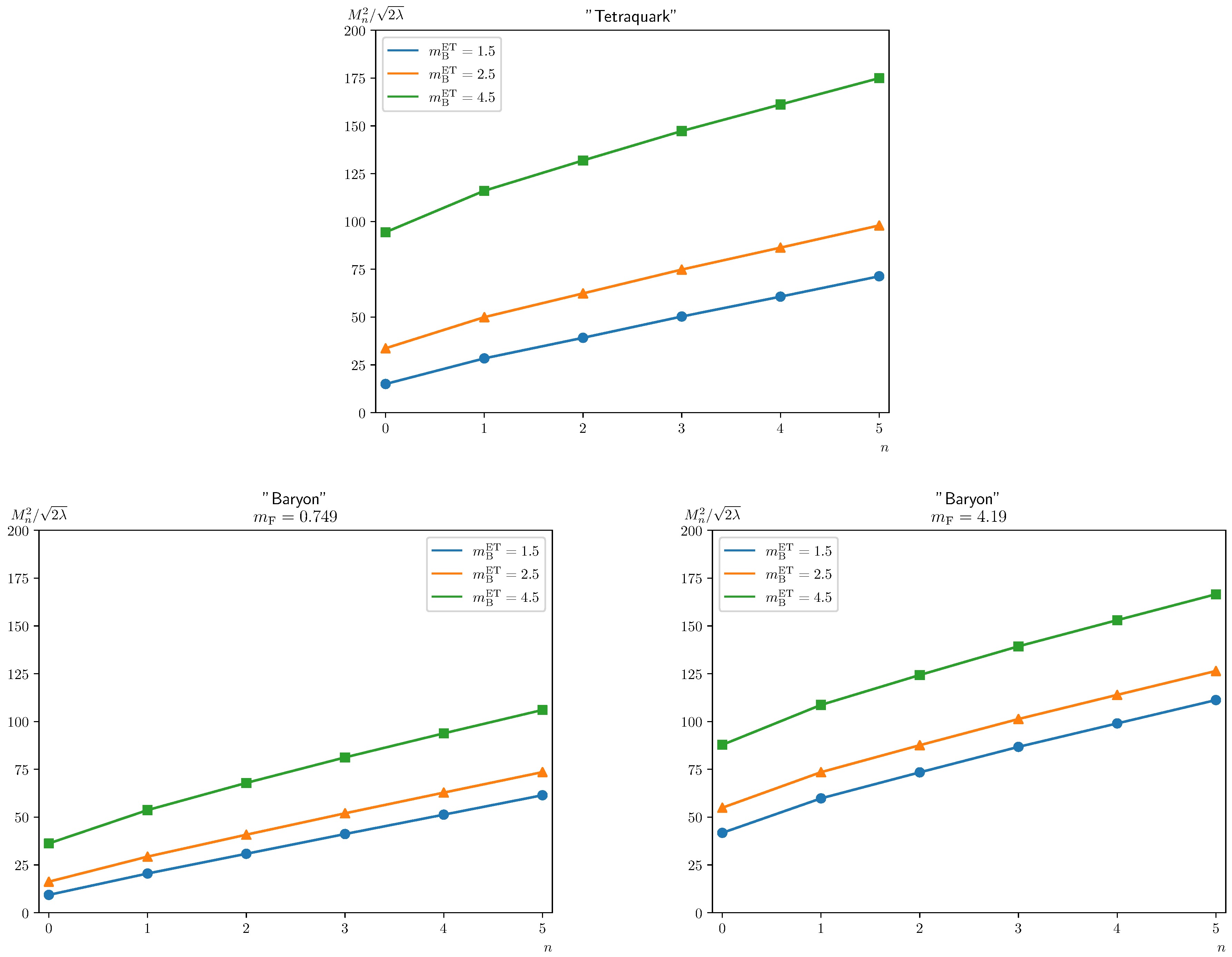
Figure 1. (color online) Mass spectra of the “tetraquark” and “baryon” with some different set of quark masses.
In passing we mention a technical nuisance, i.e., it is found that, when numerically solving the Shei-Tsao equation, the renormalized bosonic quark mass
$ m_\text{B}^\text{LC} $ can not be chosen less than unity. As pointed out in [59], such case may corresponds to a strongly coupled regime, where the the LF wave function near the endpoints is no longer real-valued.In Fig 2, we plot the equal-time and light-front (LF) meson wave functions pertaining to “tetraquark” and “baryon”, including both the ground states and the first excited states. For a “tetraquark” consisting of a single flavor of bosonic quark, the LF wave functions with even/odd n are symmetric/antisymmetric under the exchange
$ x \leftrightarrow (1-x) $ due to the charge conjugation symmetry. The LF wave functions always vanish in the endpoints$ x = 0,1 $ .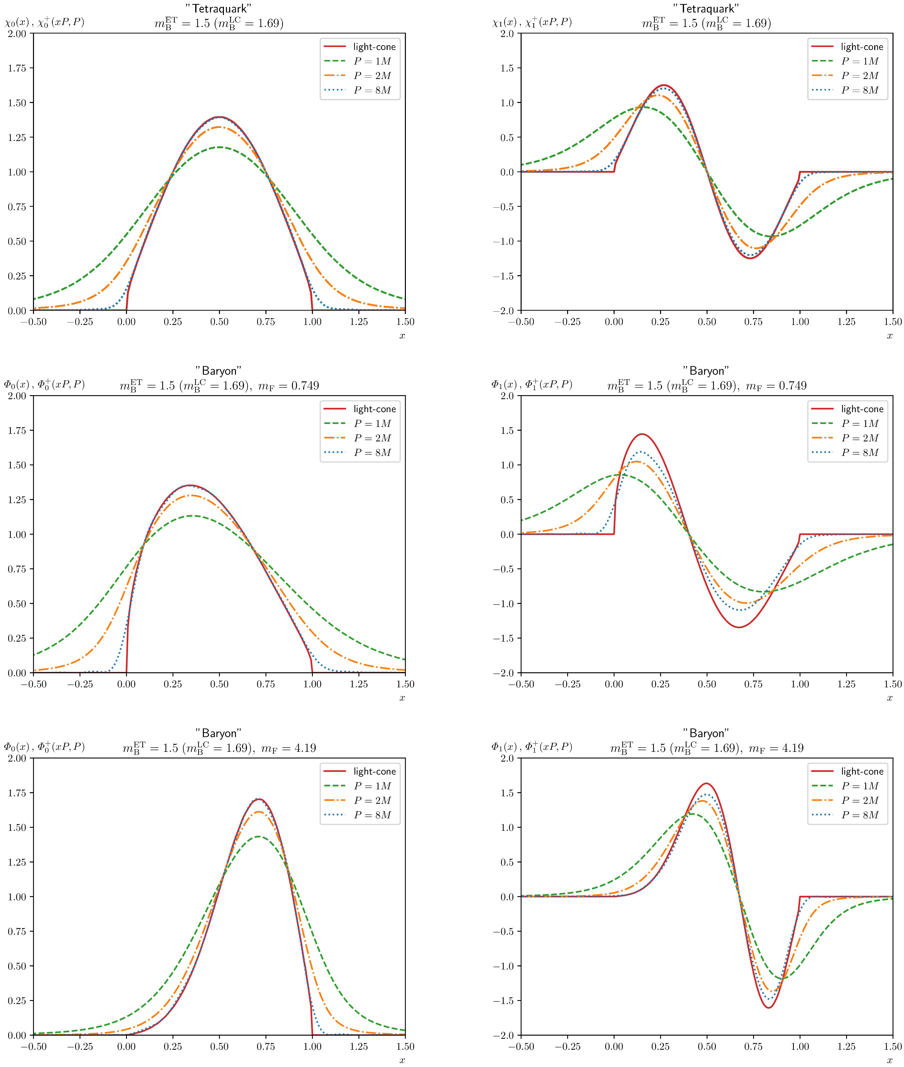
Figure 2. (color online) Profiles of the forward-moving components of the wave functions of “tetraquark” and “baryons”, viewed from different finite momentum frames. The wave functions of the ground state are shown in the left column, while those of the first excited state are shown in the right column. The solid curves represent the corresponding light-cone wave functions.
It is interesting to see how the bound-state wave functions obtained in equal-time quantization evolve with the hadron's momentum. As is evident in Fig 2, as the hadron momentum increases, the forward-moving wave functions of “tetraquark”,
$ \chi_{+} $ , and of “baryon”,$ \varPhi_{+} $ , rapidly converge to the corresponding light-cone wave functions. We have also numerically verified that, the backward-moving wave functions,$ \chi_{-} $ and$ \varPhi_{-} $ , do quickly fade away with increasing hadron momentum. This finding is identical with what is observed in the numerical study of the original 't Hooft model [23], which is compatible with the tenet of LaMET. -
The numerical solution of bound-state wave functions have been widely discussed [42–49]. We follow the approach similar to [46] for the evaluation of light-cone wave functions and the Hermite function approach [51] for the equal-time wave functions. In order to simulate the physical mesons, we set the 't Hooft coupling to be
$ \sqrt{2\lambda}=340\text{ MeV} $ , which agrees with the value of string tension in$ {\rm{QCD}}_4 $ . For notational brevity, we use$ \sqrt{2\lambda} $ as the unit of mass in the rest of this section. The mass of scalar quark is assumed to be$ m_{sc}^\text{ET}\equiv m_{\tilde{r}}=1.5 $ ($ m_{sc}^\text{LC}\equiv m_{r} $ ). As for spinor quarks, we choose the mass of strange quark as$ m_{sp}=0.749 $ and charm quark as$ m_{sp}=4.19 $ .In Fig. 1, the meson mass spectra of different quark species are illustrated as functions of the principal quantum number n. It's exhibited that the square of the meson mass is linearly related to n. This phenomenon is analogous to the Regge trajectories in the 4 dimensional QCD where n is replaced by the spin J.
Figure 1. (color online) Mass spectra of a few low-lying mesonic levels with different quark mass. To facilitate the distinction between scalar quark and spinor quark,
$ m_{\tilde{r}}=m_{sc}^\text{ET} $ .We have numerically solved the bound state wave functions for scalar QCD
$ _2 $ and hybrid QCD$ _2 $ in the axial and light-cone gauges. In the process of calculation, we found that the renormalized scalar quark mass$ m_{sc}^\text{LC} $ in the light-front cannot be less than one, which corresponds to a strongly coupled region, where the asymptotic behavior of the wave function at the boundary is not a pure real number [50].In Fig. 2, we plot the equal-time and light-front (LF) meson wave functions in scalar and hybrid QCD
$ _2 $ , considering both the ground states and the first excited states. For single-flavor mesons consist of scalar quarks, the wave functions with even/odd n are symmetric/antisymmetric under the exchange$ x \leftrightarrow (1-x) $ due to the charge conjugation symmetry. The LF wave functions always vanish in both end points$ x = 0,1 $ . For heavy quark, the LF wave function possesses a much milder rising/falling shape near the end points and is mainly distributed at moderate values of x. When the mesons momentum goes to the infinity, the equal-time wave functions$ \chi_{+} $ and$ \varPhi_{+} $ will boost to the light-front bound state equation, while the$ \chi_{-} $ and and$ \varPhi_{-} $ components rapidly dies off. This phenomenon validates the large momentum effective theory (LaMET) and reflects the normative invariance of the theory.
Figure 2. (color online) bound state equation for the bound-state and the 1st excited state.
$ \chi_n(x,P)\equiv\chi_n(p=xP,P) $ ,$ \varPhi_n(x,P)\equiv\varPhi_n(p=xP,P) $ . -
The numerical recipe of solving the BSEs in 't Hooft model has been adequately discussed in literature. We follow the approach outlined in [19] to solve the BSEs of the ''tetraquark'' and ''baryon'' in IMF, and follow the approach based on Hermite function expansion [21, 23] to solve the BSEs of the ''extotic'' hadrons in FMF.
The dimensionful 't Hooft coupling is usually taken to be
$ \sqrt{2\lambda} = 340\text{ MeV} $ , which is close to the value of string tension in$ \text{QCD}_4 $ . For simplicity, we use$ \sqrt{2\lambda} $ as the unit of the mass in the rest of this section. The renormalized mass of bosonic quark in equal-time quantization is taken to be$ m_B^\text{ET}\equiv m_{B,\tilde{r}} = 1.5 $ , which is equivalent to the one defined in LF quantization,$ m_\text{B}^\text{LC}\equiv m_{B,r} = 1.69 $ 5 . As for fermionic quarks, we choose the strange quark mass as$ m_F = 0.749 $ and charm quark mass as$ m_F = 4.19 $ [23].In Fig. 1, the mass spectra of ''tetraquark'' and ''baryon'' with different quark species are plotted against the principal quantum number n. One can observe the tendency that the squared hadron mass linearly grows with n when the principle quantum number gets large. This pattern is identical with the Regge trajectory observed in the original 't Hooft model, which is also somewhat analogous to the Regge trajectories observed in the real world, where the squared mass of the excited hadronic state linearly grows with the spin.
Figure 1. (color online) Mass spectra of the ''tetraquark'' and ''baryon'' with some different set of quark masses.
In passing we mention a technical nuisance, i.e., it is found that, when numerically solving the Shei-Tsao equation, the renormalized bosonic quark mass
$ m_\text{B}^\text{LC} $ can not be chosen less than unity. As pointed out in [54], such case may corresponds to a strongly coupled regime, where the the LF wave function near the endpoints is no longer real-valued.In Fig 2, we plot the equal-time and light-front (LF) meson wave functions pertaining to ''tetraquark'' and ''baryon'', including both the ground states and the first excited states. For a ''tetraquark'' consisting of a single flavor of bosonic quark, the LF wave functions with even/odd n are symmetric/antisymmetric under the exchange
$ x \leftrightarrow (1-x) $ due to the charge conjugation symmetry. The LF wave functions always vanish in the endpoints$ x = 0,1 $ .
Figure 2. (color online) Profiles of the forward-moving components of the wave functions of ''tetraquark'' and ''baryons'', viewed from different finite momentum frames. The wave functions of the ground state are shown in the left column, while those of the first excited state are shown in the right column. The solid curves represent the corresponding light-cone wave functions.
It is interesting to see how the bound-state wave functions obtained in equal-time quantization evolve with the hadron's momentum. As is evident in Fig 2, as the hadron momentum increases, the forward-moving wave functions of ''tetraquark'',
$ \chi_{+} $ , and of ''baryon'',$ \varPhi_{+} $ , rapidly converge to the corresponding light-cone wave functions. We have also numerically verified that, the backward-moving wave functions,$ \chi_{-} $ and$ \varPhi_{-} $ , do quickly fade away with increasing hadron momentum. This finding is identical with what is observed in the numerical study of the original 't Hooft model [23], which is compatible with the tenet of LaMET. -
In this work, we have made a comprehensive study of the extended 't Hooft model, viz., two-dimensional QCD including both fermionic and bosonic quarks in
$ N_c\to \infty $ limit. We focus on derivations of the bound-state equations pertaining to two types of hadrons, a ''tetraquark'' composed of a bosonic quark and a bosonic antiquark, and a ''baryon'' composed of a fermionic quark and bosonic antiquark. Using the Hamiltonian approach, we derive these BSEs from the perspectives of light-front and equal-time quantization, which are associated with the IMF and FMF, respectively. We confirm the known results, such as those BSEs of ''tetraquark'' in IMF [37] and in FMF [39]. We have paid special attention to the issue concerning quark mass renormalization. It is found that, the renormalized bosonic quark mass in scalar$ \text{QCD}_2 $ in light-front quantization may not coincide with that in equal-time quantization, and the relationship between these two types of renormalized quark mass is established. Moreover, for the first time we also present a diagrammatic derivation of the ''tetraquark'' BSEs in FMF.We have also confirmed the BSE of ''baryon'' in the extended 't Hooft model in IMF [50]. The main new result of this work is to derive, for the first time, the BSEs of ''baryon'' in FMF in the context of equal-time quantization.
We have also conducted a comprehensive numerical study of mass spectra of ''tetraquark'' and ''baryon''. The Regge trajectories are explicitly demonstrated. We have also obtained the profiles of the wave functions of the ground and first excited states of ''tetraquark'' and ''baryon'', viewed from different FMFs. We have numerically verified that, when the ''tetraquark'' and ''baryon'' are boosted to IMF, the forward-moving components of the bound-state wave functions approach the corresponding light-cone wave functions, and the backward-moving components fade away.
-
In this work, we have made a comprehensive study on the two-dimensional QCD, focusing on the bound-state equations for mesons composed of a scalar quark and scalar antiquark, as well as exotoic baryons composed of a fermionic quark and bosonic antiquark. These equations are obtained from both light-front quantization and equal-time quantization. Our major theoretical tool is the Hamiltonian operator approach. However, for the first time we also present a diagrammatical derivation of the mesonic bound-state equation in the equal-time quantization for scalar
$ {\rm QCD}_2 $ . We confirm the known equations for mesonic case and for the hybrid baryon in the light-front quantization, paying particular attention to the mass renormalization issue. We find that, in scalar$ {\rm{QCD}}_2 $ , the renormalized quark mass in light-front may not coincide with that in equal-time, depending on the chosen renormalization schemes. We establish the relationship between these two renormalized masses. For the first time, we also derive the bound-state equation for the exotic baryons in the equal-time quantization.We also conduct a comprehensive numerical study on the hadron spectroscopy and solving the bound-state wave functions of the ground and first-excited states. We utilize the concept of generalized functions to solve the mass-gap equation. We also explicitly verify the trend that as the hadron is boosted to infinite-momentum frame, the forward-moving bound-state wave function approach the light-front wave function.
-
In this work, we have made a comprehensive study of the extended 't Hooft model, viz., two-dimensional QCD including both fermionic and bosonic quarks in
$ N_c\to \infty $ limit. We focus on derivations of the bound-state equations pertaining to two types of hadrons, a “tetraquark” composed of a bosonic quark and a bosonic antiquark, and a “baryon” composed of a fermionic quark and bosonic antiquark. Using the Hamiltonian approach, we derive these BSEs from the perspectives of light-front and equal-time quantization, which are associated with the IMF and FMF, respectively. We confirm the known results, such as those BSEs of “tetraquark” in IMF [37] and in FMF [39]. We have paid special attention to the issue concerning quark mass renormalization. It is found that, the renormalized bosonic quark mass in scalar$ \text{QCD}_2 $ in light-front quantization may not coincide with that in equal-time quantization, and the relationship between these two types of renormalized quark mass is established. Moreover, for the first time we also present a diagrammatic derivation of the “tetraquark” BSEs in FMF.We have also confirmed the BSE of “baryon” in the extended 't Hooft model in IMF [50]. The main new result of this work is to derive, for the first time, the BSEs of “baryon” in FMF in the context of equal-time quantization.
We have also conducted a comprehensive numerical study of mass spectra of “tetraquark” and “baryon”. The Regge trajectories are explicitly demonstrated. We have also obtained the profiles of the wave functions of the ground and first excited states of “tetraquark” and “baryon”, viewed from different FMFs. We have numerically verified that, when the “tetraquark” and “baryon” are boosted to IMF, the forward-moving components of the bound-state wave functions approach the corresponding light-cone wave functions, and the backward-moving components fade away.
-
In this Appendix, we utilize the Feynman diagrammatical method to redefine the bound-state equations for scalar
$ {\rm QCD}_2 $ in equal-time quantization. -
In this Appendix, we employ the diagrammatic technique to rederive the bound-state equations of “tetraquark” in scalar
$ {\rm{QCD}}_2 $ in the context of equal-time quantization. -
In this Appendix, we employ the diagrammatic technique to rederive the bound-state equations of ''tetraquark'' in scalar
$ {\rm{QCD}}_2 $ in the context of equal-time quantization. -
To quantize scalar
$ {\rm{QCD}}_2 $ in equal-time, we adopt the axial gauge$ A^z = 0 $ and proceed by expanding the Lagrangian as follows:$ \begin{aligned}[b] {\cal{L}}_{\text{sQCD}_2} =\;& \mathrm{tr}\left(\partial_z A^0\right)^2 + \left(\partial^\mu\phi^\dagger\right)\partial_\mu\phi - m^2\phi^{\dagger}\phi \\& -i g_\mathrm{s}\left(\partial_0\phi^\dagger\right) A^0\phi + {\rm i} g_\mathrm{s}\phi^\dagger A^0\partial_0\phi + g_\mathrm{s}^2\phi^\dagger A^0A^0\phi. \end{aligned}$
(A1) The Feynman rules can be directly derived from (A1) and are summarized in Table A1. A key challenge in equal-time quantization of scalar
$ {\rm{QCD}}_2 $ , compared to its spinor counterpart, lies in the presence of seagull vertices. These vertices disrupt the rainbow-ladder topology even at leading order in the$ 1/ N_\mathrm{c} $ expansion.Building blocks Double lines Feynman rules 

$ {\dfrac{i}{\left(k^z\right)^2}} $ 

$ {\dfrac{i}{p^2 - m^2 + i\epsilon}} $ 

$ {\dfrac{i g_\mathrm{s}}{\sqrt{2}}\left(p^0 + p^{\prime0}\right)} $ 

$\dfrac{i g_{\mathrm{s}}^2}{2} $ Table A1. Original Feynman rules for sQCD2 in the axial gauge
The solution proceeds in a straightforward manner: we decompose each seagull vertex into two
$ q\bar{q}g $ vertices, and reorganize its contribution into a new term of the quark propagator between these two vertices. However, this cannot be done naively, since the Feynman rule for the$ q\bar{q}g $ vertex depends on the momenta of the two adjacent quark lines, while a term in the quark propagator only accounts for the momentum flowing through it. To address this, we must also split the$ q\bar{q}g $ vertex into different types and distribute the quark momenta into the two adjacent quark propagators separately. This process is illustrated in Fig. A1. To fully absorb the seagull vertex, it becomes necessary to introduce four distinct types of quark propagators, which are shown in Fig. A2. In retrospect, these propagators emerge quite naturally, and can, to some extent, be associated with the propagators from$ \phi^\dagger\left(y\right), -{\rm i}\pi^\dagger\left(y\right) $ to$ \phi\left(x\right), {\rm i}\pi\left(x\right) $ within the Hamiltonian formalism. The situation here is somewhat analogous though not identical to the relationship between canonical quantization and path integral quantization for the massive vector field. The contact term arising from the seagull vertex cancels out the$ \left(p^0\right)^2 $ numerator in the quark propagator, yielding the correct residue for$ p^0 $ . For convenience, we define$ \omega_p^2 \equiv \left(p^z\right)^2 + m^2 -{\rm i} \epsilon $ .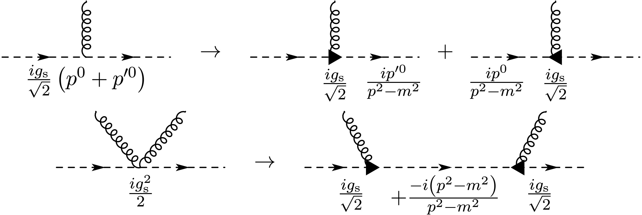
Figure A1. Modification of the Feynman rules to remove the seagull vertex.
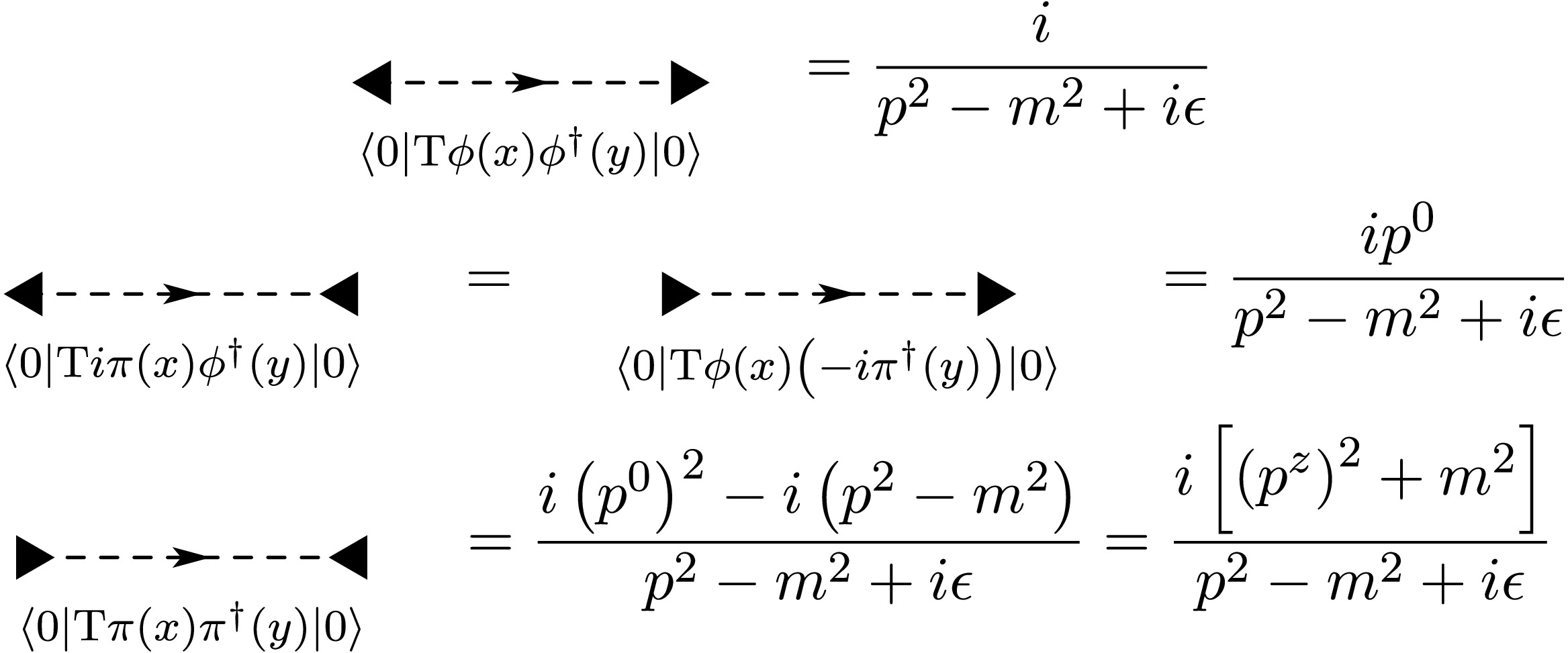
Figure A2. Modification of the quark propagators.
To streamline the calculation, we express the four quark propagators (Fig. A2) in the form of a
$ 2\times2 $ matrix:$ D^{(0)}\left(p\right) = \frac{{\rm i}\left(p^{0}\sigma_1 + {\cal{P}}_+ + \omega_p^2 {\cal{P}}_-\right)}{p^2-m^2+{\rm i}\epsilon}, $
(A2) where the projectors
$ {\cal{P}}_\pm \equiv \left(1\pm\sigma_3\right)/2 $ satisfy the orthogonality and completeness relations:$ {\cal{P}}_\pm^2 = {\cal{P}}_\pm,\quad {\cal{P}}_\pm{\cal{P}}\mp = 0,\quad {\cal{P}}_+ + {\cal{P}}_- = 1, $
(A3) and the algebra:
$\begin{aligned}[b]& \sigma_1{\cal{P}}_\pm = {\cal{P}}_\mp \sigma_1,\\&\left(X\sigma_1 + Y{\cal{P}}_+ + Z {\cal{P}}_-\right)\left(X\sigma_1 - Z{\cal{P}}_+ - Y{\cal{P}}_-\right) = X^2-YZ,\end{aligned} $
(A4) for scalar quantities
$ X,Y,Z $ . It is important to emphasize that the introduction of the Pauli σ-matrices here is unrelated to spinors. In fact, the mass dimensions of the matrix elements in (A2) are not homogeneous. However, this particular choice of matrix multiplication ensures that only terms of uniform dimension will be added within the matrix elements. The modified Feynman rules are summarized in Table A2.Building blocks Feynman rules 
$ {\dfrac{i}{\left(k^z\right)^2}} $ 
$ {\dfrac{i}{p^0\sigma_1 - \omega_p^2\mathcal{P}_{+} -\mathcal{P}_{-}}} $ 
$ {\dfrac{i g_\mathrm{s}}{\sqrt{2}}\sigma_1} $ Table A2. Modified Feynman rules for sQCD
$ _2 $ in the axial gauge. -
To quantize scalar
$ {\rm{QCD}}_2 $ in equal-time, we adopt the axial gauge$ A^z = 0 $ and proceed by expanding the Lagrangian as follows:$ \begin{aligned}[b] {\cal{L}}_{\text{sQCD}_2} =\;& \mathrm{tr}\left(\partial_z A^0\right)^2 + \left(\partial^\mu\phi^\dagger\right)\partial_\mu\phi - m^2\phi^{\dagger}\phi \\& -i g_\mathrm{s}\left(\partial_0\phi^\dagger\right) A^0\phi + i g_\mathrm{s}\phi^\dagger A^0\partial_0\phi + g_\mathrm{s}^2\phi^\dagger A^0A^0\phi. \end{aligned}$
(A1) The Feynman rules can be directly derived from (A1) and are summarized in Table A1. A key challenge in equal-time quantization of scalar
$ {\rm{QCD}}_2 $ , compared to its spinor counterpart, lies in the presence of seagull vertices. These vertices disrupt the rainbow-ladder topology even at leading order in the$ 1/ N_\mathrm{c} $ expansion.Building blocks Double lines Feynman rules $ {\dfrac{i}{\left(k^z\right)^2}} $ $ {\dfrac{i}{p^2 - m^2 + i\epsilon}} $ $ {\dfrac{i g_\mathrm{s}}{\sqrt{2}}\left(p^0 + p^{\prime0}\right)} $ $\dfrac{i g_{\mathrm{s}}^2}{2} $ Table A1. Original Feynman rules for sQCD2 in the axial gauge
The solution proceeds in a straightforward manner: we decompose each seagull vertex into two
$ q\bar{q}g $ vertices, and reorganize its contribution into a new term of the quark propagator between these two vertices. However, this cannot be done naively, since the Feynman rule for the$ q\bar{q}g $ vertex depends on the momenta of the two adjacent quark lines, while a term in the quark propagator only accounts for the momentum flowing through it. To address this, we must also split the$ q\bar{q}g $ vertex into different types and distribute the quark momenta into the two adjacent quark propagators separately. This process is illustrated in Fig. A1. To fully absorb the seagull vertex, it becomes necessary to introduce four distinct types of quark propagators, which are shown in Fig. A2. In retrospect, these propagators emerge quite naturally, and can, to some extent, be associated with the propagators from$ \phi^\dagger\left(y\right), -i\pi^\dagger\left(y\right) $ to$ \phi\left(x\right), i\pi\left(x\right) $ within the Hamiltonian formalism. The situation here is somewhat analogous though not identical to the relationship between canonical quantization and path integral quantization for the massive vector field. The contact term arising from the seagull vertex cancels out the$ \left(p^0\right)^2 $ numerator in the quark propagator, yielding the correct residue for$ p^0 $ . For convenience, we define$ \omega_p^2 \equiv \left(p^z\right)^2 + m^2 -i \epsilon $ .
Figure A1. Modification of the Feynman rules to remove the seagull vertex.
Figure A2. Modification of the quark propagators.
To streamline the calculation, we express the four quark propagators (Fig. A2) in the form of a
$ 2\times2 $ matrix:$ D^{(0)}\left(p\right) = \frac{i\left(p^{0}\sigma_1 + {\cal{P}}_+ + \omega_p^2 {\cal{P}}_-\right)}{p^2-m^2+i\epsilon}, $
(A2) where the projectors
$ {\cal{P}}_\pm \equiv \left(1\pm\sigma_3\right)/2 $ satisfy the orthogonality and completeness relations:$ {\cal{P}}_\pm^2 = {\cal{P}}_\pm,\quad {\cal{P}}_\pm{\cal{P}}\mp = 0,\quad {\cal{P}}_+ + {\cal{P}}_- = 1, $
(A3) and the algebra:
$\begin{aligned}[b]& \sigma_1{\cal{P}}_\pm = {\cal{P}}_\mp \sigma_1,\\&\left(X\sigma_1 + Y{\cal{P}}_+ + Z {\cal{P}}_-\right)\left(X\sigma_1 - Z{\cal{P}}_+ - Y{\cal{P}}_-\right) = X^2-YZ,\end{aligned} $
(A4) for scalar quantities
$ X,Y,Z $ . It is important to emphasize that the introduction of the Pauli σ-matrices here is unrelated to spinors. In fact, the mass dimensions of the matrix elements in (A2) are not homogeneous. However, this particular choice of matrix multiplication ensures that only terms of uniform dimension will be added within the matrix elements. The modified Feynman rules are summarized in Table A2.Building blocks Feynman rules $ {\dfrac{i}{\left(k^z\right)^2}} $ $ {\dfrac{i}{p^0\sigma_1 - \omega_p^2\mathcal{P}_{+} -\mathcal{P}_{-}}} $ $ {\dfrac{i g_\mathrm{s}}{\sqrt{2}}\sigma_1} $ Table A2. Modified Feynman rules for sQCD
$ _2 $ in the axial gauge. -
The s
$ {\rm QCD}_2 $ lagrangian is expanded as$ \begin{aligned}[b] \mathcal{L}_{\text{sQCD}_2} =& \mathrm{tr}\left(\partial_z A^0\right)^2 + \left(\partial^\mu\phi^\dagger\right)\partial_\mu\phi - m^2\phi^{\dagger}\phi \\ & -i g_\mathrm{s}\left(\partial_0\phi^\dagger\right) A^0\phi + i g_\mathrm{s}\phi^\dagger A^0\partial_0\phi + g_\mathrm{s}^2\phi^\dagger A^0A^0\phi. \end{aligned}\tag{A1} $

The Feynman rules can be derived directly from (88) and are shown in Table A1. The main obstacle of this approach in scalar
$ {\rm{QCD}}_2 $ compared with the case of spinor$ {\rm{QCD}}_2 $ is that the appearance of seagull vertices may mess up the rainbow-ladder topology at the leading order of$ 1/ N_\mathrm{c} $ .Building blocks Double lines Feynman rules $ {\dfrac{i}{\left(k^z\right)^2}} $ 

$ {\dfrac{i}{p^2 - m^2 + i\epsilon}} $ 

$ {\dfrac{i g_\mathrm{s}}{\sqrt{2}}\left(p^0 + p^{\prime0}\right)} $ 

$\dfrac{i g_{\mathrm{s}}^2}{2} $ 

Table A1. Original Feynman rules for sQCD2 in the axial gauge
The solution is straightforward. We break up each seagull vertex into two
$ q\bar{q}g $ vertices and reorganize its contribution into a new term of the quark propagator in between. However, this can not be done naively, since the Feynman rule of the$ q\bar{q}g $ vertex depends on the momenta of the two attached quark lines while a term in the quark propagator only knows about the momentum that flows through it. So we also need to break the$ q\bar{q}g $ vertex and move the momenta into the two attached quark propagators separately. This procedure is illustrated in Fig. A1. Note that in order to absorb the seagull vertex, we have to introduce four kinds of quark propagators, which are depicted in Fig. 2. With hindsight, these propagators are quite natural, and to some extent we can identify them with the propagators from$ \phi^\dagger\left(y\right), -i\pi^\dagger\left(y\right) $ to$ \phi\left(x\right), i\pi\left(x\right) $ in the Hamiltonian approach. The situation here is a bit similar (though not the same) to the relation between the canonical quantization and the path integral quantization of the massive vector field. The contact term from the seagull vertex cancels the$ \left(p^0\right)^2 $ numerator in the quark propagator to give the correct$ p^0 $ residue. For convenience we define$ \omega_p^2 \equiv \left(p^z\right)^2 + m^2 -i \epsilon $ .
Figure A1. Modification of the Feynman rules to remove the seagull vertex.
Figure A2. Modification of the quark propagators.
To simplify the calculation, we write the four quark propagators as a
$ 2\times2 $ matrix.$ D^{(0)}\left(p\right) = \frac{i\left(p^{0}\sigma_1 + \mathcal{P}_+ + \omega_p^2 \mathcal{P}_-\right)}{p^2-m^2+i\epsilon}, \tag{A2} $

where the projectors
$ \mathcal{P}_\pm \equiv \left(1\pm\sigma_3\right)/2 $ satisfy the orthogonality and completeness relations$ \mathcal{P}_\pm^2 = \mathcal{P}_\pm,\quad \mathcal{P}_\pm\mathcal{P}\mp = 0,\quad \mathcal{P}_+ + \mathcal{P}_- = 1, \tag{A3} $

and the following algebra
$ \sigma_1\mathcal{P}_\pm = \mathcal{P}_\mp \sigma_1,\quad \frac{\left(X\sigma_1 + Y\mathcal{P}_+ + Z \mathcal{P}_-\right)\left(X\sigma_1 - Z\mathcal{P}_+ - Y\mathcal{P}_-\right)} {X^2-YZ} = 1, \tag{A4} $

for scalars
$ X,Y,Z $ . It should be emphasized that the introduction of the Pauli σ matrices has nothing to do with spinors. In fact, the mass dimensions in (A2) don't even match. However, this particularly chosen matrix multiplication guarantees that only uniform-dimension terms in the matrix elements will be added together. The modified Feynman rules are summarized in Table A2.Building blocks Feynman rules $ {\dfrac{i}{\left(k^z\right)^2}} $ 

$ {\dfrac{i}{p^0\sigma_1 - \omega_p^2\mathcal{P}_{+} -\mathcal{P}_{-}}} $ 

$ {\dfrac{i g_\mathrm{s}}{\sqrt{2}}\sigma_1} $ 

Table A2. Modified Feynman rules for sQCD2 in the axial gauge.
-
Let the contribution of the one-particle irreducible (1PI) diagrams to the self-energy correction of quark propagator be denoted by
$ -i\Sigma\left(p\right) $ . In the large-$ N_\mathrm{c} $ limit, the dressed quark propagator$ D\left(p\right) $ is determined by the rainbow diagrams (Fig. A3). It satisfies the following recursive equations: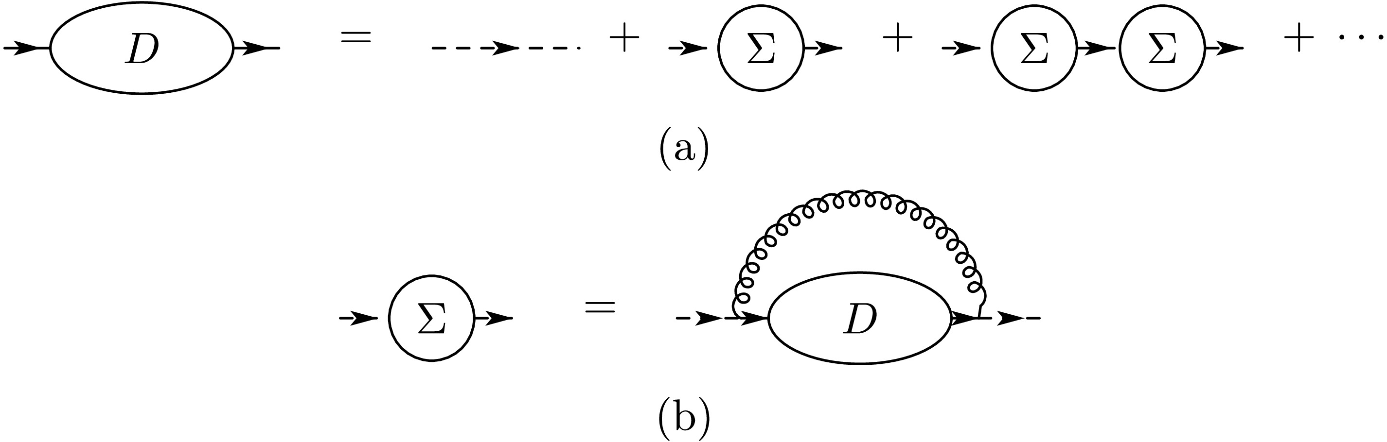
Figure A3. Dressed quark propagator in the large-
$ N_\mathrm{c} $ limit.$ D\left(p\right) = \frac{i}{p^0\sigma_1 - \omega_p^2 {\cal{P}}_+ - {\cal{P}}_- -\Sigma\left(p\right)}, $
(A5a) $ -i\Sigma\left(p\right) = \frac{-i g_\mathrm{s}^2 N_\mathrm{c}}{2} \rlap- \displaystyle {\int }\frac{d^2 k}{\left(2\pi\right)^2} \frac{\sigma_1D\left(k\right)\sigma_1}{\left(p^z-k^z\right)^2}, $
(A5b) where the following expansion has been employed:
$ \frac{1}{X - Y} = X^{-1} + X^{-1}YX^{-1} + X^{-1}YX^{-1}YX^{-1} + \cdots. $
(A6) Apparently
$ \Sigma\left(p\right) $ is independent of$ p^0 $ . The most general form is$ \Sigma\left(p\right) = A\left(p^z\right) {\cal{P}}_+ + B\left(p^z\right) {\cal{P}}_-. $
(A7) The
$ \sigma_1 $ term does not appear in (A7) because we take the principal value of the$ k^0 $ integral in (A5b) at$ k^0 = \infty $ , i.e., we take the average of the contour closed at the upper half-plane and the contour closed at the lower half-plane. The dressed quark propagator now becomes$ D\left(p\right) = i\frac{p^0\sigma_1 + \left(1+B\right){\cal{P}}_+ +\left(\omega_p^2+A\right){\cal{P}}_-} {\left(p^0\right)^2 - \left(1+B\right)\left(\omega_p^2+A\right)}. $
(A8) Introducing the following magic variables,
$ E_p^2 \equiv \frac{\omega_p^2+A}{1+B},\quad F_p^2 \equiv \left(1+B\right)\left(\omega_p^2+A\right), $
(A9) their advantage shows up immediately:
$\begin{aligned}[b] D\left(p\right) =\;& i\frac{p^0\sigma_1 + \frac{F_p}{E_p}{\cal{P}}_+ + E_p F_p {\cal{P}}_-} {\left(p^0-F_p\right)\left(p^0+F_p\right)} \\ =\;& \frac{i}{2}\left( \frac{\sigma_1 + \frac{1}{E_p}{\cal{P}}_+ + E_p{\cal{P}}_-} {p^0 - F_p + i\epsilon} + \frac{\sigma_1 - \frac{1}{E_p}{\cal{P}}_+ - E_p{\cal{P}}_-} {p^0 + F_p - i\epsilon} \right), \end{aligned} $
(A10) where we have made assumptions that
$ \omega_p^2+A>0 $ ,$ 1+B>0 $ . Substituting (A10) into (95b), we find$ A\left(p^z\right) {\cal{P}}_+ + B\left(p^z\right) {\cal{P}}_- = \frac{\lambda}{2} \rlap- \displaystyle {\int } dk^z \frac{E_k{\cal{P}}_+ + \frac{1}{E_k}{\cal{P}}_-}{\left(p^z-k^z\right)^2}. $
(A11) Matching the coefficients of
$ {\cal{P}} $ and utilizing (A9), we find the equations for$ E_p $ and$ F_p $ :$\begin{aligned}[b] F_p =\;& \frac{1}{E_p} \left( \omega_p^2 + \frac{\lambda}{2} \rlap- \displaystyle {\int } dk^z \frac{E_k}{\left(p^z-k^z\right)^2} \right) \\=\;& E_p \left( 1 + \frac{\lambda}{2} \rlap- \displaystyle {\int } dk^z \frac{1}{\left(p^z-k^z\right)^2}\frac{1}{E_k} \right).\end{aligned} $
(A12) (From (A12) one can identify
$ E_p $ with$ E_p $ in the Hamiltonian approach and$ F_p $ with$ \Pi^+\left(p\right) $ .)Explicit calculation shows that the numerators of (A10) can be decomposed into outer products of two vectors:
$ \frac{\sigma_1 + \dfrac{1}{E_p}{\cal{P}}_+ + E_p{\cal{P}}_-}{2} = \xi\left(p\right) \tilde{\xi}\left(p\right)\sigma_1, $
(A13a) $ \frac{\sigma_1 - \dfrac{1}{E_p}{\cal{P}}_+ - E_p{\cal{P}}_-}{2} = \eta\left(p\right) \tilde{\eta}\left(p\right)\sigma_1, $
(A13b) where
$ \xi\left(p\right) = \frac{1}{\sqrt{2}}\left(1, E_p\right)^ \mathrm{T}, \quad \tilde{\xi}\left(p\right) = \frac{1}{\sqrt{2}}\left(1, 1/E_p\right), $
(A14a) $ \eta\left(p\right) = \frac{1}{\sqrt{2}}\left(1, -E_p\right)^ \mathrm{T}, \quad \tilde{\eta}\left(p\right) = \frac{1}{\sqrt{2}}\left(1, -1/E_p\right). $
(A14b) The dressed quark propagator can then be written as
$ D\left(p\right) = \frac{i\xi\left(p\right)\tilde{\xi}\left(p\right)\sigma_1} {p^0 - F_p + i\epsilon} + \frac{i\eta\left(p\right)\tilde{\eta}\left(p\right)\sigma_1} {p^0 + F_p - i\epsilon}. $
(A15) -
Let the contribution of one-particle irreducible (1PI) diagrams in the self-energy correction of quark propagator be given by
$ -i\Sigma\left(p\right) $ . The dressed quark propagator$ D\left(p\right) $ in the large-$ N_\mathrm{c} $ limit is governed by the rainbow diagrams (Fig. A3). It satisfies the recursive equations:
Figure A3. Dressed quark propagator in the large-
$ N_\mathrm{c} $ limit.$ D\left(p\right) = \frac{i}{p^0\sigma_1 - \omega_p^2 \mathcal{P}_+ - \mathcal{P}_- -\Sigma\left(p\right)}, \tag{A5a}$

$ -i\Sigma\left(p\right) = \frac{-i g_\mathrm{s}^2 N_\mathrm{c}}{2} {\rlap{—} \int }\frac{d^2 k}{\left(2\pi\right)^2} \frac{\sigma_1D\left(k\right)\sigma_1}{\left(p^z-k^z\right)^2}, \tag{A5b} $

where we have used
$ \frac{1}{X - Y} = X^{-1} + X^{-1}YX^{-1} + X^{-1}YX^{-1}YX^{-1} + \cdots. \tag{A6} $

Apparently
$ \Sigma\left(p\right) $ is independent of$ p^0 $ . The most general form is$ \Sigma\left(p\right) = A\left(p^z\right) \mathcal{P}_+ + B\left(p^z\right) \mathcal{P}_-. \tag{A7} $

The
$ \sigma_1 $ term does not appear in (A7) because we take the principal value of the$ k^0 $ integral in (A5b) at$ k^0=\infty $ , i.e., we take the average of the contour closed at the upper half-plane and the contour closed at the lower half-plane. The dressed quark propagator now becomes$ D\left(p\right) = i\frac{p^0\sigma_1 + \left(1+B\right)\mathcal{P}_+ +\left(\omega_p^2+A\right)\mathcal{P}_-} {\left(p^0\right)^2 - \left(1+B\right)\left(\omega_p^2+A\right)}. \tag{A8} $

Introducing the following magic variables,
$ E_p^2 \equiv \frac{\omega_p^2+A}{1+B},\quad F_p^2 \equiv \left(1+B\right)\left(\omega_p^2+A\right), \tag{A9} $

their advantage shows up immediately:
$ \begin{aligned}[b] D\left(p\right) =& i\frac{p^0\sigma_1 + \dfrac{F_p}{E_p}\mathcal{P}_+ + E_p F_p \mathcal{P}_-} {\left(p^0-F_p\right)\left(p^0+F_p\right)} \\ =& \frac{i}{2}\left( \frac{\sigma_1 + \dfrac{1}{E_p}\mathcal{P}_+ + E_p\mathcal{P}_-} {p^0 - F_p + i\epsilon} + \frac{\sigma_1 - \dfrac{1}{E_p}\mathcal{P}_+ - E_p\mathcal{P}_-} {p^0 + F_p - i\epsilon} \right), \end{aligned}\tag{A10} $

where we have made assumptions that
$ \omega_p^2+A>0 $ ,$ 1+B>0 $ . Substituting (A10) into (A5b), we find$ A\left(p^z\right) \mathcal{P}_+ + B\left(p^z\right) \mathcal{P}_- = \frac{\lambda}{2} {\rlap{—} \int } dk^z \frac{E_k\mathcal{P}_+ + \dfrac{1}{E_k}\mathcal{P}_-}{\left(p^z-k^z\right)^2}. \tag{A11} $

Matching the coefficients of
$ \mathcal{P} $ and utilizing (96), we find the equations for$ E_p $ and$ F_p $ :$ \begin{aligned}[b] F_p &= \frac{1}{E_p} \left( \omega_p^2 + \frac{\lambda}{2} {\rlap{—} \int } dk^z \frac{E_k}{\left(p^z-k^z\right)^2} \right) \\& = E_p \left( 1 + \frac{\lambda}{2} {\rlap{—} \int } dk^z \frac{1}{\left(p^z-k^z\right)^2}\frac{1}{E_k} \right). \end{aligned}\tag{A12} $

(From (A12) one can identify
$ E_p $ with$ E_p $ in the Hamiltonian approach and$ F_p $ with$ \Pi^+\left(p\right) $ .)Explicit calculation shows that the numerators of (A10) can be decomposed into outer products of two vectors:
$ \frac{\sigma_1 + \dfrac{1}{E_p}\mathcal{P}_+ + E_p\mathcal{P}_-}{2} = \xi\left(p\right) \tilde{\xi}\left(p\right)\sigma_1, \tag{A13a} $

$ \frac{\sigma_1 - \dfrac{1}{E_p}\mathcal{P}_+ - E_p\mathcal{P}_-}{2} = \eta\left(p\right) \tilde{\eta}\left(p\right)\sigma_1, \tag{A13b} $

where
$ \xi\left(p\right) = \frac{1}{\sqrt{2}}\left(1, E_p\right)^ \mathrm{T},\quad \tilde{\xi}\left(p\right) = \frac{1}{\sqrt{2}}\left(1, 1/E_p\right), \tag{A14a} $

$ \eta\left(p\right) = \frac{1}{\sqrt{2}}\left(1, -E_p\right)^ \mathrm{T},\quad \tilde{\eta}\left(p\right) = \frac{1}{\sqrt{2}}\left(1, -1/E_p\right). \tag{A14b} $

The dressed quark propagator can then be written as
$ D\left(p\right) = \frac{i\xi\left(p\right)\tilde{\xi}\left(p\right)\sigma_1} {p^0 - F_p + i\epsilon} + \frac{i\eta\left(p\right)\tilde{\eta}\left(p\right)\sigma_1} {p^0 + F_p - i\epsilon}. \tag{A15} $

-
Let the contribution of the one-particle irreducible (1PI) diagrams to the self-energy correction of quark propagator be denoted by
$ -{\rm i}\Sigma\left(p\right) $ . In the large-$ N_\mathrm{c} $ limit, the dressed quark propagator$ D\left(p\right) $ is determined by the rainbow diagrams (Fig. A3). It satisfies the following recursive equations:
Figure A3. Dressed quark propagator in the large-
$ N_\mathrm{c} $ limit.$ D\left(p\right) = \frac{{\rm i}}{p^0\sigma_1 - \omega_p^2 {\cal{P}}_+ - {\cal{P}}_- -\Sigma\left(p\right)}, $
(A5a) $ -{\rm i}\Sigma\left(p\right) = \frac{-{\rm i} g_\mathrm{s}^2 N_\mathrm{c}}{2} \rlap— \displaystyle {\int }\frac{{\rm d}^2 k}{\left(2\pi\right)^2} \frac{\sigma_1D\left(k\right)\sigma_1}{\left(p^z-k^z\right)^2}, $
(A5b) where the following expansion has been employed:
$ \frac{1}{X - Y} = X^{-1} + X^{-1}YX^{-1} + X^{-1}YX^{-1}YX^{-1} + \cdots. $
(A6) Apparently
$ \Sigma\left(p\right) $ is independent of$ p^0 $ . The most general form is$ \Sigma\left(p\right) = A\left(p^z\right) {\cal{P}}_+ + B\left(p^z\right) {\cal{P}}_-. $
(A7) The
$ \sigma_1 $ term does not appear in (A7) because we take the principal value of the$ k^0 $ integral in (A5b) at$ k^0 = \infty $ , i.e., we take the average of the contour closed at the upper half-plane and the contour closed at the lower half-plane. The dressed quark propagator now becomes$ D\left(p\right) = {\rm i}\frac{p^0\sigma_1 + \left(1+B\right){\cal{P}}_+ +\left(\omega_p^2+A\right){\cal{P}}_-} {\left(p^0\right)^2 - \left(1+B\right)\left(\omega_p^2+A\right)}. $
(A8) Introducing the following magic variables,
$ E_p^2 \equiv \frac{\omega_p^2+A}{1+B},\quad F_p^2 \equiv \left(1+B\right)\left(\omega_p^2+A\right), $
(A9) their advantage shows up immediately:
$\begin{aligned}[b] D\left(p\right) =\;& {\rm i}\frac{p^0\sigma_1 + \frac{F_p}{E_p}{\cal{P}}_+ + E_p F_p {\cal{P}}_-} {\left(p^0-F_p\right)\left(p^0+F_p\right)} \\ =\;& \frac{{\rm i}}{2}\left( \frac{\sigma_1 + \frac{1}{E_p}{\cal{P}}_+ + E_p{\cal{P}}_-} {p^0 - F_p + {\rm i}\epsilon} + \frac{\sigma_1 - \frac{1}{E_p}{\cal{P}}_+ - E_p{\cal{P}}_-} {p^0 + F_p - {\rm i}\epsilon} \right), \end{aligned} $
(A10) where we have made assumptions that
$ \omega_p^2+A>0 $ ,$ 1+B>0 $ . Substituting (A10) into (95b), we find$ A\left(p^z\right) {\cal{P}}_+ + B\left(p^z\right) {\cal{P}}_- = \frac{\lambda}{2} \rlap— \displaystyle {\int } {\rm d}k^z \frac{E_k{\cal{P}}_+ + \frac{1}{E_k}{\cal{P}}_-}{\left(p^z-k^z\right)^2}. $
(A11) Matching the coefficients of
$ {\cal{P}} $ and utilizing (A9), we find the equations for$ E_p $ and$ F_p $ :$\begin{aligned}[b] F_p =\;& \frac{1}{E_p} \left( \omega_p^2 + \frac{\lambda}{2} \rlap— \displaystyle {\int } {\rm d}k^z \frac{E_k}{\left(p^z-k^z\right)^2} \right) \\=\;& E_p \left( 1 + \frac{\lambda}{2} \rlap— \displaystyle {\int } {\rm d}k^z \frac{1}{\left(p^z-k^z\right)^2}\frac{1}{E_k} \right).\end{aligned} $
(A12) (From (A12) one can identify
$ E_p $ with$ E_p $ in the Hamiltonian approach and$ F_p $ with$ \Pi^+\left(p\right) $ .)Explicit calculation shows that the numerators of (A10) can be decomposed into outer products of two vectors:
$ \frac{\sigma_1 + \dfrac{1}{E_p}{\cal{P}}_+ + E_p{\cal{P}}_-}{2} = \xi\left(p\right) \tilde{\xi}\left(p\right)\sigma_1, $
(A13a) $ \frac{\sigma_1 - \dfrac{1}{E_p}{\cal{P}}_+ - E_p{\cal{P}}_-}{2} = \eta\left(p\right) \tilde{\eta}\left(p\right)\sigma_1, $
(A13b) where
$ \xi\left(p\right) = \frac{1}{\sqrt{2}}\left(1, E_p\right)^ \mathrm{T}, \quad \tilde{\xi}\left(p\right) = \frac{1}{\sqrt{2}}\left(1, 1/E_p\right), $
(A14a) $ \eta\left(p\right) = \frac{1}{\sqrt{2}}\left(1, -E_p\right)^ \mathrm{T}, \quad \tilde{\eta}\left(p\right) = \frac{1}{\sqrt{2}}\left(1, -1/E_p\right). $
(A14b) The dressed quark propagator can then be written as
$ D\left(p\right) = \frac{{\rm i}\xi\left(p\right)\tilde{\xi}\left(p\right)\sigma_1} {p^0 - F_p + {\rm i}\epsilon} + \frac{{\rm i}\eta\left(p\right)\tilde{\eta}\left(p\right)\sigma_1} {p^0 + F_p - {\rm i}\epsilon}. $
(A15) -
In the large-
$ N_\mathrm{c} $ limit, The meson-$ q\bar{q} $ vertex$ \Gamma\left(p;q\right) $ satisfies the following Bethe-Salpeter equation (Fig. A4):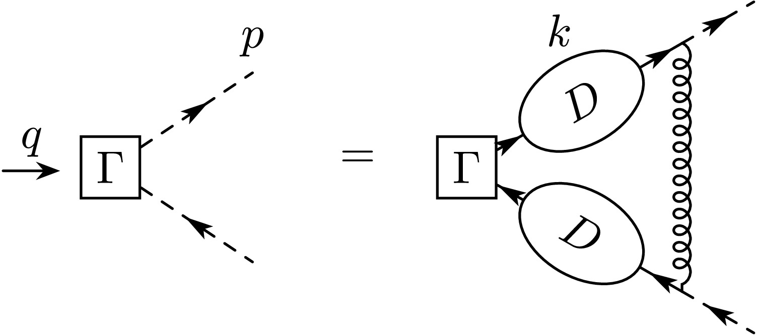
Figure A4. Meson-
$ q\bar{q} $ vertex in the large-$ N_\mathrm{c} $ limit.$ \begin{aligned}[b]\Gamma\left(p; q\right) =\;& \frac{-i g_\mathrm{s}^2 N_\mathrm{c}}{2} \rlap- \displaystyle {\int }\frac{d^2 k}{\left(2\pi\right)^2} \frac{1}{\left(p^z - k^z\right)^2} \sigma_1\\&\times D\left(k\right)\Gamma\left(k; q\right)D\left(k-q\right)\sigma_1.\end{aligned} $
(A16) $ \Gamma\left(p;q\right) $ is independent of$ p^0 $ , so we can perform the$ k^0 $ integration:$ {\cal{I}}\left(k; q\right) \equiv \int\frac{dk^0}{2\pi} D\left(k\right)\Gamma\left(k; q\right) D\left(k-q\right). $
(A17) The interpretation of
$ {\cal{I}}\left(k; q\right) $ at the matrix-element level is$ {\cal{I}}\left(k; q\right) = \int dz\;e^{-ik^z z} \langle{\Omega}\vert \Phi\left(0, z\right) \Phi^\dagger\left(0, 0\right)\vert{M_n\left(q\right)}\rangle, $
(A18) where
$ \Phi\left(x\right) = \left(\phi\left(x\right), i\pi\left(x\right)\right)^ \mathrm{T} $ and$ M_n $ is the n-th excitation of the bound states. Among the four projections of$ D\left(k\right) $ and$ D\left(k-q\right) $ , only two of them give nonzero residues. We arrive at$ \begin{aligned}[b] {\cal{I}}\left(k;q\right) =\;& \frac{ \xi\left(k\right)\left[ -i \tilde{\xi}\left(k\right)\sigma_1\Gamma\left(k;q\right)\eta\left(k-q\right) \right]\tilde{\eta}\left(k-q\right)\sigma_1 }{q^0_n - F\left(k-q\right)-F\left(k\right) + i\epsilon} \\ & + \frac{ \eta\left(k\right)\left[ -i \tilde{\eta}\left(k\right)\sigma_1\Gamma\left(k;q\right)\xi\left(k-q\right) \right]\tilde{\xi}\left(k-q\right)\sigma_1 }{- q^0_n - F\left(k-q\right)-F\left(k\right) + i\epsilon} \\ \equiv \;&-\chi^+_n\left(k^z;q^z\right) \sqrt{\frac{E_{k-q}}{E_k}} \xi\left(k\right)\tilde{\eta}\left(k-q\right)\sigma_1 \\ & - \chi^-_n\left(k^z;q^z\right) \sqrt{\frac{E_{k-q}}{E_k}} \eta\left(k\right)\tilde{\xi}\left(k-q\right)\sigma_1. \end{aligned} $
(A19) From now on we drop the superscript z in spacial momenta for simplicity. Substituting (A16) into (A19), we get
$ \begin{aligned}[b]& \left[q^0_n - F\left(p-q\right)-F\left(p\right)\right]\chi^+_n\left(p;q\right) = -\lambda \rlap- \displaystyle {\int } \frac{d k}{\left(p-k\right)^2} \sqrt{\frac{E_pE_{k-q}}{E_kE_{p-q}}} \times\Big[ \tilde{\xi}\left(p\right)\xi\left(k\right)\tilde{\eta}\left(k-q\right)\eta\left(p-q\right) \chi^+_n\left(k;q\right) \\ &\quad + \tilde{\xi}\left(p\right)\eta\left(k\right)\tilde{\xi}\left(k-q\right)\eta\left(p-q\right) \chi^-_n\left(k;q\right) \Big], \end{aligned} $
(A20a) $ \begin{aligned}[b]& \left[-q^0_n - F\left(p-q\right)-F\left(p\right)\right]\chi^-_n\left(p;q\right) = -\lambda \rlap- \displaystyle {\int } \frac{d k}{\left(p-k\right)^2} \sqrt{\frac{E_pE_{k-q}}{E_kE_{p-q}}} \times\Big[ \tilde{\eta}\left(p\right)\eta\left(k\right)\tilde{\xi}\left(k-q\right)\xi\left(p-q\right) \chi^-_n\left(k;q\right)\\ &\quad + \tilde{\eta}\left(p\right)\xi\left(k\right)\tilde{\eta}\left(k-q\right)\xi\left(p-q\right) \chi^+_n\left(k;q\right) \Big]. \end{aligned} $
(A20b) Using the fact that
$ \tilde{\xi}\left(p\right)\xi\left(k\right) = \tilde{\eta}\left(p\right)\eta\left(k\right) = \frac{E_p + E_k}{2E_p}, $
(A21a) $ \tilde{\xi}\left(p\right)\eta\left(k\right) = \tilde{\eta}\left(p\right)\xi\left(k\right) = \frac{E_p - E_k}{2E_p}, $
(A21b) and defining
$ f_\pm\left(p, k\right) \equiv \frac{E_k \pm E_p}{\sqrt{E_pE_k}}, $
(A22a) $ S_\pm\left(p, k; q\right) \equiv f_\pm\left(p,k\right)f_\pm\left(p-q,k-q\right), $
(A22b) the bound state equations can be written as
$ \begin{aligned}[b]& \left[q^0_n - F\left(p-q\right)-F\left(p\right)\right]\chi^+_n\left(p;q\right) = -\frac{\lambda}{4} \rlap- \displaystyle {\int } \frac{d k}{\left(p-k\right)^2} \\ &\quad \times\left[ S_+\left(p, k; q\right) \chi^+_n\left(k;q\right) - S_-\left(p, k; q\right) \chi^-_n\left(k;q\right) \right], \end{aligned} $
(A23a) $ \begin{aligned}[b]& \left[-q^0_n - F\left(p-q\right)-F\left(p\right)\right]\chi^-_n\left(p;q\right) = -\frac{\lambda}{4} \rlap- \displaystyle {\int } \frac{d k}{\left(p-k\right)^2} \\&\quad \times\left[ S_+\left(p, k; q\right) \chi^-_n\left(k;q\right) - S_-\left(p, k; q\right) \chi^+_n\left(k;q\right) \right]. \end{aligned} $
(A23b) These equations are equivalent to (52) with
$ F \equiv \Pi^+ $ . -
In the large-
$ N_\mathrm{c} $ limit, The meson-$ q\bar{q} $ vertex$ \Gamma\left(p;q\right) $ satisfies the following Bethe-Salpeter equation (Fig. A4):
Figure A4. Meson-
$ q\bar{q} $ vertex in the large-$ N_\mathrm{c} $ limit.$ \begin{aligned}[b]\Gamma\left(p; q\right) =\;& \frac{-{\rm i} g_\mathrm{s}^2 N_\mathrm{c}}{2} \rlap— \displaystyle {\int }\frac{{\rm d}^2 k}{\left(2\pi\right)^2} \frac{1}{\left(p^z - k^z\right)^2} \sigma_1\\&\times D\left(k\right)\Gamma\left(k; q\right)D\left(k-q\right)\sigma_1.\end{aligned} $
(A16) $ \Gamma\left(p;q\right) $ is independent of$ p^0 $ , so we can perform the$ k^0 $ integration:$ {\cal{I}}\left(k; q\right) \equiv \int\frac{{\rm d}k^0}{2\pi} D\left(k\right)\Gamma\left(k; q\right) D\left(k-q\right). $
(A17) The interpretation of
$ {\cal{I}}\left(k; q\right) $ at the matrix-element level is$ {\cal{I}}\left(k; q\right) = \int {\rm d}z\;{\rm e}^{{\rm -i}k^z z} \langle{\Omega}\vert \Phi\left(0, z\right) \Phi^\dagger\left(0, 0\right)\vert{M_n\left(q\right)}\rangle, $
(A18) where
$ \Phi\left(x\right) = \left(\phi\left(x\right), {\rm i}\pi\left(x\right)\right)^ \mathrm{T} $ and$ M_n $ is the n-th excitation of the bound states. Among the four projections of$ D\left(k\right) $ and$ D\left(k-q\right) $ , only two of them give nonzero residues. We arrive at$ \begin{aligned}[b] {\cal{I}}\left(k;q\right) =\;& \frac{ \xi\left(k\right)\left[ -{\rm i} \tilde{\xi}\left(k\right)\sigma_1\Gamma\left(k;q\right)\eta\left(k-q\right) \right]\tilde{\eta}\left(k-q\right)\sigma_1 }{q^0_n - F\left(k-q\right)-F\left(k\right) + {\rm i}\epsilon} \\ & + \frac{ \eta\left(k\right)\left[ -{\rm i} \tilde{\eta}\left(k\right)\sigma_1\Gamma\left(k;q\right)\xi\left(k-q\right) \right]\tilde{\xi}\left(k-q\right)\sigma_1 }{- q^0_n - F\left(k-q\right)-F\left(k\right) + {\rm i}\epsilon} \\ \equiv \;&-\chi^+_n\left(k^z;q^z\right) \sqrt{\frac{E_{k-q}}{E_k}} \xi\left(k\right)\tilde{\eta}\left(k-q\right)\sigma_1 \\ & - \chi^-_n\left(k^z;q^z\right) \sqrt{\frac{E_{k-q}}{E_k}} \eta\left(k\right)\tilde{\xi}\left(k-q\right)\sigma_1. \end{aligned} $
(A19) From now on we drop the superscript z in spacial momenta for simplicity. Substituting (A16) into (A19), we get
$ \begin{aligned}[b]& \left[q^0_n - F\left(p-q\right)-F\left(p\right)\right]\chi^+_n\left(p;q\right) = -\lambda \rlap— \displaystyle {\int } \frac{{\rm d} k}{\left(p-k\right)^2} \sqrt{\frac{E_pE_{k-q}}{E_kE_{p-q}}} \times\Big[ \tilde{\xi}\left(p\right)\xi\left(k\right)\tilde{\eta}\left(k-q\right)\eta\left(p-q\right) \chi^+_n\left(k;q\right) \\ &\quad + \tilde{\xi}\left(p\right)\eta\left(k\right)\tilde{\xi}\left(k-q\right)\eta\left(p-q\right) \chi^-_n\left(k;q\right) \Big], \end{aligned} $
(A20a) $ \begin{aligned}[b]& \left[-q^0_n - F\left(p-q\right)-F\left(p\right)\right]\chi^-_n\left(p;q\right) = -\lambda \rlap— \displaystyle {\int } \frac{{\rm d} k}{\left(p-k\right)^2} \sqrt{\frac{E_pE_{k-q}}{E_kE_{p-q}}} \times\Big[ \tilde{\eta}\left(p\right)\eta\left(k\right)\tilde{\xi}\left(k-q\right)\xi\left(p-q\right) \chi^-_n\left(k;q\right)\\ &\quad + \tilde{\eta}\left(p\right)\xi\left(k\right)\tilde{\eta}\left(k-q\right)\xi\left(p-q\right) \chi^+_n\left(k;q\right) \Big]. \end{aligned} $
(A20b) Using the fact that
$ \tilde{\xi}\left(p\right)\xi\left(k\right) = \tilde{\eta}\left(p\right)\eta\left(k\right) = \frac{E_p + E_k}{2E_p}, $
(A21a) $ \tilde{\xi}\left(p\right)\eta\left(k\right) = \tilde{\eta}\left(p\right)\xi\left(k\right) = \frac{E_p - E_k}{2E_p}, $
(A21b) and defining
$ f_\pm\left(p, k\right) \equiv \frac{E_k \pm E_p}{\sqrt{E_pE_k}}, $
(A22a) $ S_\pm\left(p, k; q\right) \equiv f_\pm\left(p,k\right)f_\pm\left(p-q,k-q\right), $
(A22b) the bound state equations can be written as
$ \begin{aligned}[b]& \left[q^0_n - F\left(p-q\right)-F\left(p\right)\right]\chi^+_n\left(p;q\right) = -\frac{\lambda}{4} \rlap— \displaystyle {\int } \frac{{\rm d} k}{\left(p-k\right)^2} \\ &\quad \times\left[ S_+\left(p, k; q\right) \chi^+_n\left(k;q\right) - S_-\left(p, k; q\right) \chi^-_n\left(k;q\right) \right], \end{aligned} $
(A23a) $ \begin{aligned}[b]& \left[-q^0_n - F\left(p-q\right)-F\left(p\right)\right]\chi^-_n\left(p;q\right) = -\frac{\lambda}{4} \rlap— \displaystyle {\int } \frac{{\rm d} k}{\left(p-k\right)^2} \\&\quad \times\left[ S_+\left(p, k; q\right) \chi^-_n\left(k;q\right) - S_-\left(p, k; q\right) \chi^+_n\left(k;q\right) \right]. \end{aligned} $
(A23b) These equations are equivalent to (52) with
$ F \equiv \Pi^+ $ . -
In the large-
$ N_\mathrm{c} $ limit, The meson-$ q\bar{q} $ vertex$ \Gamma\left(p;q\right) $ satisfies the following Bethe-Salpeter equation (Fig. A4):
Figure A4. Meson-
$ q\bar{q} $ vertex in the large-$ N_\mathrm{c} $ limit.$ \Gamma\left(p; q\right) = \frac{-i g_\mathrm{s}^2 N_\mathrm{c}}{2} {\rlap{—} \int }\frac{d^2 k}{\left(2\pi\right)^2} \frac{1}{\left(p^z - k^z\right)^2} \sigma_1D\left(k\right)\Gamma\left(k; q\right)D\left(k-q\right)\sigma_1. \tag{A16} $

$ \Gamma\left(p;q\right) $ is independent of$ p^0 $ , so we can perform the$ k^0 $ integration:$ \mathcal{I}\left(k; q\right) \equiv \int\frac{dk^0}{2\pi} D\left(k\right)\Gamma\left(k; q\right) D\left(k-q\right). \tag{A17} $

The interpretation of
$ \mathcal{I}\left(k; q\right) $ at the matrix-element level is$ \mathcal{I}\left(k; q\right) = \int dz\;e^{-ik^z z} \langle{\Omega}\vert \Phi\left(0, z\right) \Phi^\dagger\left(0, 0\right)\vert{M_n\left(q\right)}\rangle, \tag{A18} $

where
$ \Phi\left(x\right) = \left(\phi\left(x\right), i\pi\left(x\right)\right)^ \mathrm{T} $ and$ M_n $ is the n-th excitation of the bound states. Among the four projections of$ D\left(k\right) $ and$ D\left(k-q\right) $ , only two of them give nonzero residues. We arrive at$ \begin{aligned}[b] \mathcal{I}\left(k;q\right) =& \frac{ \xi\left(k\right)\left[ -i \tilde{\xi}\left(k\right)\sigma_1\Gamma\left(k;q\right)\eta\left(k-q\right) \right]\tilde{\eta}\left(k-q\right)\sigma_1 }{q^0_n - F\left(k-q\right)-F\left(k\right) + i\epsilon} \\ & + \frac{ \eta\left(k\right)\left[ -i \tilde{\eta}\left(k\right)\sigma_1\Gamma\left(k;q\right)\xi\left(k-q\right) \right]\tilde{\xi}\left(k-q\right)\sigma_1 }{- q^0_n - F\left(k-q\right)-F\left(k\right) + i\epsilon} \\ \equiv& -\chi^+_n\left(k^z;q^z\right) \sqrt{\frac{E_{k-q}}{E_k}} \xi\left(k\right)\tilde{\eta}\left(k-q\right)\sigma_1 \\ & - \chi^-_n\left(k^z;q^z\right) \sqrt{\frac{E_{k-q}}{E_k}} \eta\left(k\right)\tilde{\xi}\left(k-q\right)\sigma_1. \end{aligned}\tag{A19} $

From now on we drop the superscript z in spacial momenta for simplicity. Substituting (103) into (106), we get
$ \begin{aligned}[b] &\left[q^0_n - F\left(p-q\right)-F\left(p\right)\right]\chi^+_n\left(p;q\right) \\ =& -\lambda {\rlap{—} \int } \frac{d k}{\left(p-k\right)^2} \sqrt{\frac{E_pE_{k-q}}{E_kE_{p-q}}} \\& \times\Big[ \tilde{\xi}\left(p\right)\xi\left(k\right)\tilde{\eta}\left(k-q\right)\eta\left(p-q\right) \chi^+_n\left(k;q\right) \\ & + \tilde{\xi}\left(p\right)\eta\left(k\right)\tilde{\xi}\left(k-q\right)\eta\left(p-q\right) \chi^-_n\left(k;q\right) \Big], \end{aligned}\tag{A20a} $

$ \begin{aligned}[b] &\left[-q^0_n - F\left(p-q\right)-F\left(p\right)\right]\chi^-_n\left(p;q\right) \\ =& -\lambda {\rlap{—} \int } \frac{d k}{\left(p-k\right)^2} \sqrt{\frac{E_pE_{k-q}}{E_kE_{p-q}}} \\ & \times\Big[ \tilde{\eta}\left(p\right)\eta\left(k\right)\tilde{\xi}\left(k-q\right)\xi\left(p-q\right) \chi^-_n\left(k;q\right) \\ & + \tilde{\eta}\left(p\right)\xi\left(k\right)\tilde{\eta}\left(k-q\right)\xi\left(p-q\right) \chi^+_n\left(k;q\right) \Big]. \end{aligned}\tag{A20b} $

Using the fact that
$ \tilde{\xi}\left(p\right)\xi\left(k\right) = \tilde{\eta}\left(p\right)\eta\left(k\right)= \frac{E_p + E_k}{2E_p},\tag{A21a}$

$ \tilde{\xi}\left(p\right)\eta\left(k\right) = \tilde{\eta}\left(p\right)\xi\left(k\right) = \frac{E_p - E_k}{2E_p}, \tag{A21b}$

and defining
$ f_\pm\left(p, k\right) \equiv \frac{E_k \pm E_p}{\sqrt{E_pE_k}}, \tag{A22a} $

$ S_\pm\left(p, k; q\right) \equiv f_\pm\left(p,k\right)f_\pm\left(p-q,k-q\right), \tag{A22b} $

the bound state equations can be written as
$ \begin{aligned}[b] &\left[q^0_n - F\left(p-q\right)-F\left(p\right)\right]\chi^+_n\left(p;q\right) = -\frac{\lambda}{4} {\rlap{—} \int } \frac{d k}{\left(p-k\right)^2} \\&\quad \times\left[ S_+\left(p, k; q\right) \chi^+_n\left(k;q\right) - S_-\left(p, k; q\right) \chi^-_n\left(k;q\right) \right], \end{aligned}\tag{A23a} $

$ \begin{aligned}[b] &\left[-q^0_n - F\left(p-q\right)-F\left(p\right)\right]\chi^-_n\left(p;q\right) = -\frac{\lambda}{4} {\rlap{—} \int } \frac{d k}{\left(p-k\right)^2} \\ &\quad \times\left[ S_+\left(p, k; q\right) \chi^-_n\left(k;q\right) - S_-\left(p, k; q\right) \chi^+_n\left(k;q\right) \right]. \end{aligned}\tag{A23b} $

This equation is equivalent to (52).
-
In this appendix, we discuss some subtle issues about the mass renormalization in the scalar
$ {\rm{QCD}}_2 $ , in both equal-time and light-front quantization. We start from the equal-time quantization, and examine the asymptotic behavior of$ E_k $ and$ \Pi^+ $ in the large momentum limit.The integrals appearing in
$ \Pi^\pm $ defined in (36) as$ k\to\infty $ can be calculated with the method of regions [55]. There are two regions of the integration variable$ k_1 $ : 1)$ m_{\tilde{r}} \sim \left|k_1\right| \ll k $ ; 2)$ m_{\tilde{r}} \ll \left|k_1\right| \sim k $ . We divide the integration regions, expand the integrand according to the different scaling of each region:$\begin{aligned}[b]& \rlap— \displaystyle {\int } {\rm d}k_{1}\left( \frac{\dfrac{E_{k_1}}{E_k}\pm\dfrac{E_k}{E_{k_1}}}{(k+k_1)^{2}} -\frac{E_{k_1}}{E_k}\frac{1}{k_1^2} \right) \\\approx\;& \frac{1}{k} \rlap— \displaystyle {\int }_{\left|k_1\right|<\Lambda} {\rm d}k_{1} \left(\pm\frac{1}{E_{k_1}}-\frac{E_{k_1}}{k_1^2}\right) \\ &+ \rlap— \displaystyle {\int }_{\left|k_1\right|>\Lambda} {\rm d}k_1\left( \frac{\dfrac{\left|k_1\right|}{k}\pm\dfrac{k}{\left|k_1\right|}}{\left(k+k_1\right)^2} -\frac{1}{k\left|k_1\right|} \right), \end{aligned}$
(B1) where
$ m_{\tilde{r}}\ll\Lambda\ll k $ . For$ \Pi^+ $ , the bounds of each region can be extended to the whole momentum space since the asymptotic λ dependence of each region cancels each other:$ \begin{aligned}[b]&\rlap— \displaystyle {\int } {\rm d}k_{1}\left( \frac{\dfrac{E_{k_1}}{E_k}+\dfrac{E_k}{E_{k_1}}}{(k+k_1)^{2}} -\frac{E_{k_1}}{E_k}\frac{1}{k_1^2} \right) \\\approx\;& \frac{1}{k}\left[ \rlap— \displaystyle {\int } {\rm d}k_{1} \left(\frac{1}{E_{k_1}}-\frac{E_{k_1}}{k_1^2}\right) - 4 \right].\end{aligned} $
(B2) For
$ \Pi^- $ , the integral is divergent for each region, but the divergences cancel each other in the sum of two regions:$\begin{aligned}[b]& \rlap— \displaystyle {\int } {\rm d}k_{1}\left( \frac{\dfrac{E_{k_1}}{E_k}-\dfrac{E_k}{E_{k_1}}}{(k+k_1)^{2}} -\frac{E_{k_1}}{E_k}\frac{1}{k_1^2} \right) \\\approx\;& \lim\limits_{\Lambda/k_1\to\infty} \frac{1}{k} \left[ \rlap— \displaystyle {\int }_{-\Lambda}^{\Lambda} {\rm d}k_1 \left(-\frac{1}{E_{k_1}}-\frac{E_{k_1}}{k_1^2}\right) - 4 \ln\frac{k}{\Lambda} \right].\end{aligned} $
(B3) Define
$ k_0 $ as$ 4\ln k_{0} \equiv \lim\limits_{\Lambda/k_1\to\infty} \rlap— \displaystyle {\int }_{-\Lambda}^{\Lambda} {\rm d}k_1 \left(-\frac{1}{E_{k_1}}-\frac{E_{k_1}}{k_1^2}\right) + 4\ln\Lambda. $
(B4) The asymptotic behavior of
$ E_{k} $ can be derived from (41) as$ E_k \approx k+\frac{1}{k}\left(\frac{m_{\tilde{r}}^{2}}{2} -\lambda\ln\frac{k}{k_0}\right). $
(B5) The value of
$ E_k $ still can not be determined solely from (B5) since$ k_0 $ depends recursively on the functional form of$ E_{k_1} $ . Fortunately, however, when substituting (B5) into$ \Pi^+ $ , the$ k_0 $ dependence cancels and we arrive at$ \Pi^+\left(k\right) \approx k+\frac{m_{\tilde{r}}^{2}}{2k} +\frac{\lambda}{4k}\left[ \rlap— \displaystyle {\int } {\rm d}k_1 \left(\frac{1}{E_{k_1}}-\frac{E_{k_1}}{k_1^2}\right)-4\right], $
(B6) By relabeling the momenta
$ k = xP $ in (52) and taking the large P limit, one finds that (52) approaches (28). The relation between the renormalized masses$ m_r $ and$ m_{\tilde{r}} $ can be determined by matching the two equations:$ m_{\tilde{r}}^2 + \frac{\lambda}{2} \rlap— \displaystyle {\int } {\rm d}k_1 \left(\frac{1}{E_{k_1}}-\frac{E_{k_1}}{k_1^2}\right) = m_r^2. $
(B7) It is important to note that the relation between the equal-time renormalized mass and the light-front renormalized mass is scheme-dependent. Had we instead chosen another equal-time renormalized mass
$ m_{\hat{r}}^{2} = m^2+\frac{\lambda}{2}\int {\rm d}k_1\frac{1}{E_{k_1}}, $
(B8) we would have found that
$ m_{\hat{r}} = m_r $ . -
In this appendix, we discuss some subtle issue about the mass renormalization in the scalar
$ {\rm QCD}_2 $ , in both equal-time and light-front quantization. We start from the equal-time quantization, and examine the asymptotic behavior of$ E_k $ and$ \Pi^+ $ in the large meson momentum limit.The integrals appear in
$ \Pi^\pm $ defined in (36) as$ k\to\infty $ can be calculated with the method of regions [36]. There are two regions of the integration variable$ k_1 $ : 1)$ m_{\tilde{r}} \sim \left|k_1\right| \ll k $ ; 2)$ m_{\tilde{r}} \ll \left|k_1\right| \sim k $ . We divide the integration regions, expand the integrand according to the different scaling of each region:$ \begin{aligned}[b]& {\rlap{—} \int } dk_{1}\left( \frac{\dfrac{E_{k_1}}{E_k}\pm\dfrac{E_k}{E_{k_1}}}{(k+k_1)^{2}} -\frac{E_{k_1}}{E_k}\frac{1}{k_1^2} \right) \\\approx &\frac{1}{k} {\rlap{—} \int }_{\left|k_1\right|<\Lambda} dk_{1} \left(\pm\frac{1}{E_{k_1}}-\frac{E_{k_1}}{k_1^2}\right) \\ &+ {\rlap{—} \int }_{\left|k_1\right|>\Lambda} dk_1\left( \frac{\dfrac{\left|k_1\right|}{k}\pm\dfrac{k}{\left|k_1\right|}}{\left(k+k_1\right)^2} -\frac{1}{k\left|k_1\right|} \right), \end{aligned}\tag{B1} $

where
$ m_{\tilde{r}}\ll\Lambda\ll k $ . For$ \Pi^+ $ , the bounds of each region can be extended to the whole momentum space since the asymptotic Λ dependence of each region cancels each other:$ {\rlap{—} \int } dk_{1} \left( \frac{\dfrac{E_{k_1}}{E_k}+\dfrac{E_k}{E_{k_1}}}{(k+k_1)^{2}} -\frac{E_{k_1}}{E_k}\frac{1}{k_1^2} \right) \approx \frac{1}{k}\left[ {\rlap{—} \int } dk_{1} \left(\frac{1}{E_{k_1}}-\frac{E_{k_1}}{k_1^2}\right) - 4 \right]. \tag{B2} $

For
$ \Pi^- $ , the integral is divergent for each region:$ \begin{aligned}[b]& {\rlap{—} \int } dk_{1}\left( \frac{\dfrac{E_{k_1}}{E_k}-\dfrac{E_k}{E_{k_1}}}{(k+k_1)^{2}} -\frac{E_{k_1}}{E_k}\frac{1}{k_1^2} \right) \\ \approx& \lim\limits_{\Lambda/k_1\to\infty} \frac{1}{k} \left[ {\rlap{—} \int }_{-\Lambda}^{\Lambda} dk_1 \left(-\frac{1}{E_{k_1}}-\frac{E_{k_1}}{k_1^2}\right) - 4 \ln\frac{k}{\Lambda} \right]. \end{aligned}\tag{B3} $

Define
$ k_0 $ as$ 4\ln k_{0} \equiv \lim\limits_{\Lambda/k_1\to\infty} {\rlap{—} \int }_{-\Lambda}^{\Lambda} dk_1 \left(-\frac{1}{E_{k_1}}-\frac{E_{k_1}}{k_1^2}\right) + 4\ln\Lambda. \tag{B4} $

the asymptotic behavior of
$ E_{k} $ can be derived from (41) as$ E_k approx k+\frac{1}{k}\left(\frac{m_{\tilde{r}}^{2}}{2} -\lambda\ln\frac{k}{k_0}\right). \tag{B5} $

The value of
$ E_k $ still can not be read directly from (125) since$ k_0 $ depends recursively on the functional form of$ E_{k_1} $ . Fortunately, however, when substituting (125) into$ \Pi^+ $ , the$ k_0 $ dependence cancels and we arrive at$ \Pi^+\left(k\right) \approx k+\frac{m_{\tilde{r}}^{2}}{2k} +\frac{\lambda}{4k}\left[ {\rlap{—} \int } dk_1 \left(\frac{1}{E_{k_1}}-\frac{E_{k_1}}{k_1^2}\right)-4\right], \tag{B6} $

Relabelling the momenta
$ k=xP $ in (52), and taking the large P limit, one finds that (52) approaches (28). The relation between the renormalization masses$ m_r $ and$ m_{\tilde{r}} $ can be found by matching two equations:$ m_{\tilde{r}}^2 + \frac{\lambda}{2} {\rlap{—} \int } dk_1 \left(\frac{1}{E_{k_1}}-\frac{E_{k_1}}{k_1^2}\right) = m_r^2. \tag{B7} $

Note that this relation is scheme dependent. Had we chosen the equal-time renormalized mass
$ m_{\hat{r}}^{2} = m^2+\frac{\lambda}{2}\int dk_1\frac{1}{E_{k_1}}, \tag{B8}$

we would get
$ m_{\hat{r}} = m_r $ . -
In this appendix, we discuss some subtle issues about the mass renormalization in the scalar
$ {\rm{QCD}}_2 $ , in both equal-time and light-front quantization. We start from the equal-time quantization, and examine the asymptotic behavior of$ E_k $ and$ \Pi^+ $ in the large momentum limit.The integrals appearing in
$ \Pi^\pm $ defined in (36) as$ k\to\infty $ can be calculated with the method of regions [60]. There are two regions of the integration variable$ k_1 $ : 1)$ m_{\tilde{r}} \sim \left|k_1\right| \ll k $ ; 2)$ m_{\tilde{r}} \ll \left|k_1\right| \sim k $ . We divide the integration regions, expand the integrand according to the different scaling of each region:$\begin{aligned}[b]& \rlap- \displaystyle {\int } dk_{1}\left( \frac{\dfrac{E_{k_1}}{E_k}\pm\dfrac{E_k}{E_{k_1}}}{(k+k_1)^{2}} -\frac{E_{k_1}}{E_k}\frac{1}{k_1^2} \right) \\\approx\;& \frac{1}{k} \rlap- \displaystyle {\int }_{\left|k_1\right|<\Lambda} dk_{1} \left(\pm\frac{1}{E_{k_1}}-\frac{E_{k_1}}{k_1^2}\right) \\ &+ \rlap- \displaystyle {\int }_{\left|k_1\right|>\Lambda} dk_1\left( \frac{\dfrac{\left|k_1\right|}{k}\pm\dfrac{k}{\left|k_1\right|}}{\left(k+k_1\right)^2} -\frac{1}{k\left|k_1\right|} \right), \end{aligned}$
(B1) where
$ m_{\tilde{r}}\ll\Lambda\ll k $ . For$ \Pi^+ $ , the bounds of each region can be extended to the whole momentum space since the asymptotic λ dependence of each region cancels each other:$ \begin{aligned}[b]&\rlap- \displaystyle {\int } dk_{1}\left( \frac{\dfrac{E_{k_1}}{E_k}+\dfrac{E_k}{E_{k_1}}}{(k+k_1)^{2}} -\frac{E_{k_1}}{E_k}\frac{1}{k_1^2} \right) \\\approx\;& \frac{1}{k}\left[ \rlap- \displaystyle {\int } dk_{1} \left(\frac{1}{E_{k_1}}-\frac{E_{k_1}}{k_1^2}\right) - 4 \right].\end{aligned} $
(B2) For
$ \Pi^- $ , the integral is divergent for each region, but the divergences cancel each other in the sum of two regions:$\begin{aligned}[b]& \rlap- \displaystyle {\int } dk_{1}\left( \frac{\dfrac{E_{k_1}}{E_k}-\dfrac{E_k}{E_{k_1}}}{(k+k_1)^{2}} -\frac{E_{k_1}}{E_k}\frac{1}{k_1^2} \right) \\\approx\;& \lim\limits_{\Lambda/k_1\to\infty} \frac{1}{k} \left[ \rlap- \displaystyle {\int }_{-\Lambda}^{\Lambda} dk_1 \left(-\frac{1}{E_{k_1}}-\frac{E_{k_1}}{k_1^2}\right) - 4 \ln\frac{k}{\Lambda} \right].\end{aligned} $
(B3) Define
$ k_0 $ as$ 4\ln k_{0} \equiv \lim\limits_{\Lambda/k_1\to\infty} \rlap- \displaystyle {\int }_{-\Lambda}^{\Lambda} dk_1 \left(-\frac{1}{E_{k_1}}-\frac{E_{k_1}}{k_1^2}\right) + 4\ln\Lambda. $
(B4) The asymptotic behavior of
$ E_{k} $ can be derived from (41) as$ E_k \approx k+\frac{1}{k}\left(\frac{m_{\tilde{r}}^{2}}{2} -\lambda\ln\frac{k}{k_0}\right). $
(B5) The value of
$ E_k $ still can not be determined solely from (B5) since$ k_0 $ depends recursively on the functional form of$ E_{k_1} $ . Fortunately, however, when substituting (B5) into$ \Pi^+ $ , the$ k_0 $ dependence cancels and we arrive at$ \Pi^+\left(k\right) \approx k+\frac{m_{\tilde{r}}^{2}}{2k} +\frac{\lambda}{4k}\left[ \rlap- \displaystyle {\int } dk_1 \left(\frac{1}{E_{k_1}}-\frac{E_{k_1}}{k_1^2}\right)-4\right], $
(B6) By relabeling the momenta
$ k = xP $ in (52) and taking the large P limit, one finds that (52) approaches (28). The relation between the renormalized masses$ m_r $ and$ m_{\tilde{r}} $ can be determined by matching the two equations:$ m_{\tilde{r}}^2 + \frac{\lambda}{2} \rlap- \displaystyle {\int } dk_1 \left(\frac{1}{E_{k_1}}-\frac{E_{k_1}}{k_1^2}\right) = m_r^2. $
(B7) It is important to note that the relation between the equal-time renormalized mass and the light-front renormalized mass is scheme-dependent. Had we instead chosen another equal-time renormalized mass
$ m_{\hat{r}}^{2} = m^2+\frac{\lambda}{2}\int dk_1\frac{1}{E_{k_1}}, $
(B8) we would have found that
$ m_{\hat{r}} = m_r $ .
Solving bound-state equations in QCD2 with bosonic and fermionic quarks
- Received Date: 2023-04-28
- Available Online: 2026-04-15
Abstract: We investigate the bound-state equations (BSEs) in two-dimensional QCD in the $ N_{\rm{c}}\to \infty$ limit, viewed from both the infinite momentum frame (IMF) and the finite momentum frame (FMF). The BSE of a meson in the original 't Hooft model, viz., spinor QCD2 containing only fermionc quarks, has been extensively studied in literature. In this work, we focus on the BSEs pertaining to two types of ''exotic'' hadrons, a ''tetraquark'' which is composed of a bosonic quark and bosonic antiquark, and a ''baryon'' which is composed of a bosonic antiquark and a fermionic quark. Utilizing the Hamiltonian approach, we derive the corresponding BSEs for both types of ''exotic'' hadrons, from the perspectives of the light-front and equal-time quantization, and confirm the known results. The recently available BSEs for ''tetraquark'' in FMF has also been recovered with the aid of the diagrammatic approach. For the first time we also present the BSEs of a ''baryon'' in FMF in the extended 't Hooft model. By solving various BSEs numerically, we obtain the mass spectra pertaining to ''tetraquark'' and ''baryon'' and the corresponding bound-state wave functions of the lowest-lying states. It is numerically demonstrated that, when a ''tetraquark'' or ''baryon'' is continuously boosted, the forward-moving component of the bound-state wave function approaches the corresponding light-cone wave function, while the backward-moving component fades away.


 DownLoad: