An Unitary Coupled-Channel Approach to J/ψ Radiative decay to Pseudoscalar Pairs

Quantum Chromodynamics (QCD) constitutes the fundamental theory of strong interactions [1], presents one of the most profound challenges in modern physics: the mechanism by which quarks and gluons form hadrons. While perturbative methods successfully describe high-energy regimes, the low-energy domain remains intractable due to nonperturbative phenomena such as color confinement. Recent experimental discoveries of new hadrons [2] have further challenged the conventional quark model, where mesons are understood as quark-antiquark pairs and baryons as three-quark systems. These observations provide critical insights into exotic resonance dynamics and nonperturbative QCD, yet our understanding remains limited by sparse statistical data and incomplete amplitude parameterizations [3]. Many candidates are observed exclusively in single production or decay channels, necessitating rigorous constraints on reaction amplitudes to reduce systematic uncertainties.

Traditional Breit-Wigner (BW) parameterizations suffice for narrow, isolated resonances but fail for overlapping states or those near thresholds. In such cases, preserving fundamental amplitude properties—unitarity (from probability conservation) and analyticity (from causality)—requires more sophisticated coupled-channel frameworks [4]. The K-matrix formalism [5], for instance, enforces unitarity through real matrix elements but suffers from limitations: its fixed matrix structure struggles with new channels, and parameter uncertainties degrade accuracy for high-statistics data. Crucially, it neglects energy-dependent of the real part of self-energy corrections, leading to inconsistencies in lineshape descriptions and pole extractions [6−8].

A key objective in QCD is the search for glueballs—exotic states dominated by gluonic interactions—which directly probe non-Abelian gauge dynamics. Radiative $ J/\psi $ decays to pseudoscalar meson pairs offer a unique window into glueball production, as demonstrated by extensive BESIII studies [9, 10]. These gluon-rich processes are ideal for identifying scalar and tensor glueball candidates [11], though challenges persist due to broad, overlapping resonances and flavor-blind gluonic decays that populate multiple channels [12]. Conventional BW methods are inadequate for resolving these complexities.

In this work, we develop a unitary coupled-channel amplitude for $ J/\psi\to\gamma ab $ (where a and b are pseudoscalars), incorporating: two-pseudoscalar rescattering via coupled-channel Lippmann-Schwinger (LS) equations [13−16], intermediate meson-photon couplings ($ a\bar{X}\to\gamma b $), and energy-dependent self-energies absent in K-matrix approaches. Our framework avoids the pitfalls of BW and K-matrix methods by embedding unitary two-body amplitudes directly into the decay process, enabling unbiased resonance property extraction from experimental data. We validate the model’s efficacy using toy calculations and demonstrate its application to $ J/\psi \to \gamma K_{S}K_{S} $.

The rest of this paper is structured as follows. In the following section, we outline the model construction and formalism. Section III will present the calculation of $ J/\psi \to \gamma K_{S}K_{S} $ process as an example by using this formalism. We include concluding remarks and a discussion in Section IV.

We analyze the process $ J/\psi \to \gamma ab $, where a, b denote pseudoscalar mesons, incorporating two coupled-channel effects:

1. Rescattering $ ab \to ab $: Dominated by intermediate resonances ($ XY $) originating from bare states.

2. Rescattering $ \bar{X}a \to \bar{X}'b $: Assumes constant decay widths for $ \bar{X} $ (which couples to $ \gamma a $) and neglects $ \bar{X} $'s coupled channels.

These approximations are justified because:

● Electromagnetic interactions (e.g., photon rescattering) are negligible compared to strong interactions.

● Including $ \bar{X} $'s strong decays would require a three-body formalism at least, breaking two-body unitarity—a reasonable trade-off for this work.

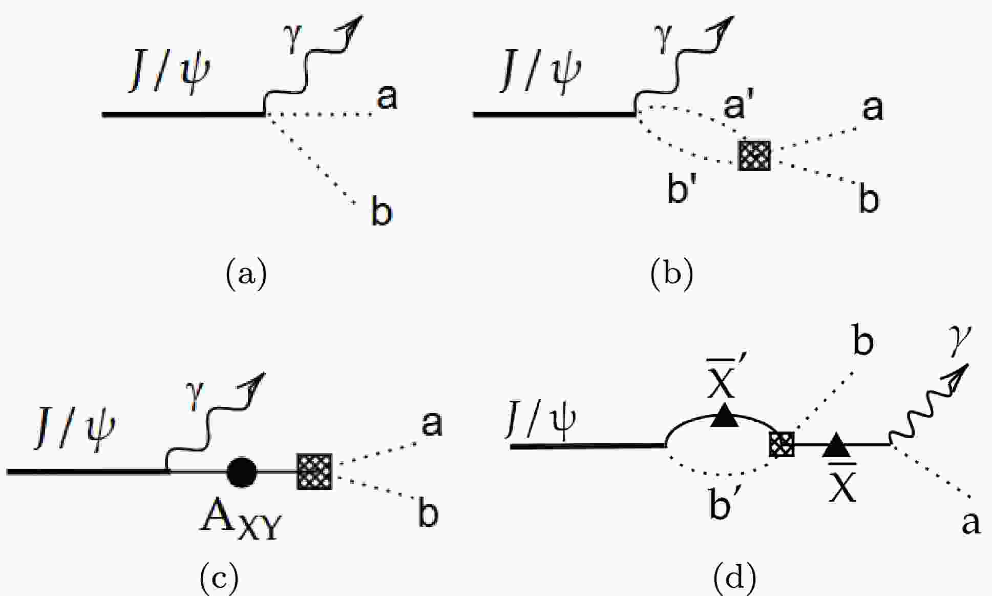
The decay processes $ J/\psi \to \gamma ab $ can be classified into the following four categories as illustrated in Fig. 1. In Fig. 1(a), the process corresponds to a direct three-body decay governed by the vertex of $ J/\psi \gamma ab $. The contribution of rescattering $ a'b'\to ab $ is included in Fig. 1(b). It is worth mentioning that the first vertex shares with that in the diagram (a), and the rescattering contribution is described by the full T-matrix of $ a'b'\to ab $ which will be discussed in the next section in detail. In Fig. 1(c), it refers to the bare state X. $ J/\psi $ first radiative decays to bare state X, and then X will couple to the final $ ab $ state. Here we need a new vertex of $ J/\psi\gamma X $, a full propagator matrix of bare states X, denoted as $ A_{XY} $, and a dressed vertex of $ Xab $. Importantly, the propagator matrix and the dressed vertex of $ Xab $ are both determined by the T-matrix of the rescattering $ a'b'\to ab $. At last, in Fig. 1(d), we show the contribution of the rescattering of $ \bar{X}a $, which is totally independent of the previous three mechanisms. Conventional isobar models (e.g., BW) only include Fig. 1(c), violating unitarity for overlapping resonances.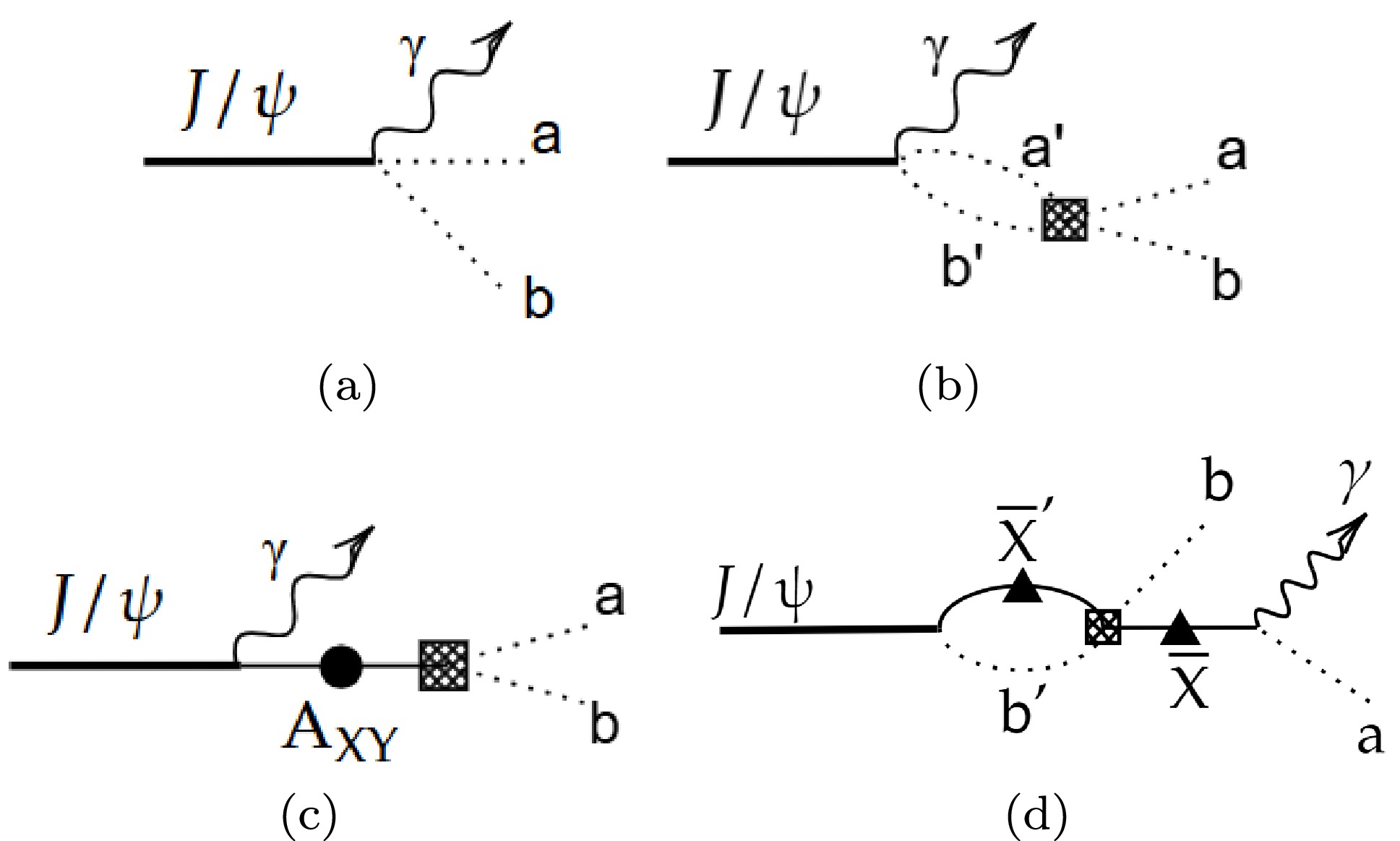

Figure 1.  The diagrams for the four categories of reactions. In this paper, pseudoscalar mesons are represented by dashed lines, and bare states by solid lines. Grid-patterned boxes denote coupling vertices associated with specific initial and final states, while solid black circles depict propagators modified through self-energy corrections. Solid black triangles symbolize propagators of bare states with parameter-adjusted properties.

The S-matrix connects the initial and final states, which encodes the probabilities of transitions between them. Since S-matrix satisfies the unitarity for the conservation of probability, i.e., $ S^\dagger S=1 $, it is well defined and can be expressed through phase shifts and inelasticities, which can be extracted from the experimental observables. Furthermore, the T-matrix calculated from the interaction vertices based on the theoretical models can also be used to derive the S-matrix through the standard scattering theory. However, under different notation, the connection between them may differ. In this paper, we use the following definition for the $ 2\to2 $ process[17],

where f and i are for the final and initial states, respectively. The $ \rho_i(E) $ is the states density of the channel i for two bodies system, given as

where the $ k_{i} $ is defined as the on-shell momentum for channel i, i.e., $ E=\sqrt{k^2_{i}+m_{i1}^2}+\sqrt{k^2_{i}+m_{i2}^2} $, and E is the total energy in their CM frame. Then the differential cross section between two channels can be expressed as follows,

where $ \bar{\sum} $ is for the average the spin states of initial state i and summation of the spin states of finial state f. In addition, for the differential decay width, it is expressed as,

Typically, the T-matrix defined here has a factor different from usual covariant amplitude $ {\cal{M}} $ defined in Particle group data [1] as follows,

for $ 2\to2 $, and

for $ 1\to 2 $. It is related to the definition of the LS equation to solve the T-matrix. Here the symbol $ fi $ refers to the final states and initial states, while the $ T_{fi} $ is the T-matrix elements.

The LS equation, defined in the center-mass system (CMS) of the final two-body system, is formulated as follows for the fixed partial wave denoted by angular momentum L,

where, the potential $ \tilde{V}^L $ between two coupled channels includes contributions from bare states with spins $ J=L $ and the direct vertices. And here α and β refer to the final and initial states since the two sides of re-scattering are one of the considered channels. The $ T^L_{\alpha\beta} $ is the partial wave amplitude for $ \alpha\to\beta $ with angular monument L. The on-shell energy $ \omega_{\gamma} $ of the given channel is defined as $ \omega_{\gamma}(q)=\sqrt{m_1^2+q^2}+\sqrt{m_2^2+q^2} $. The corresponding diagrams for the processes $ 2\to2 $ and $ 1\to2 $ are shown in Figs. 2(a) and (b), respectively.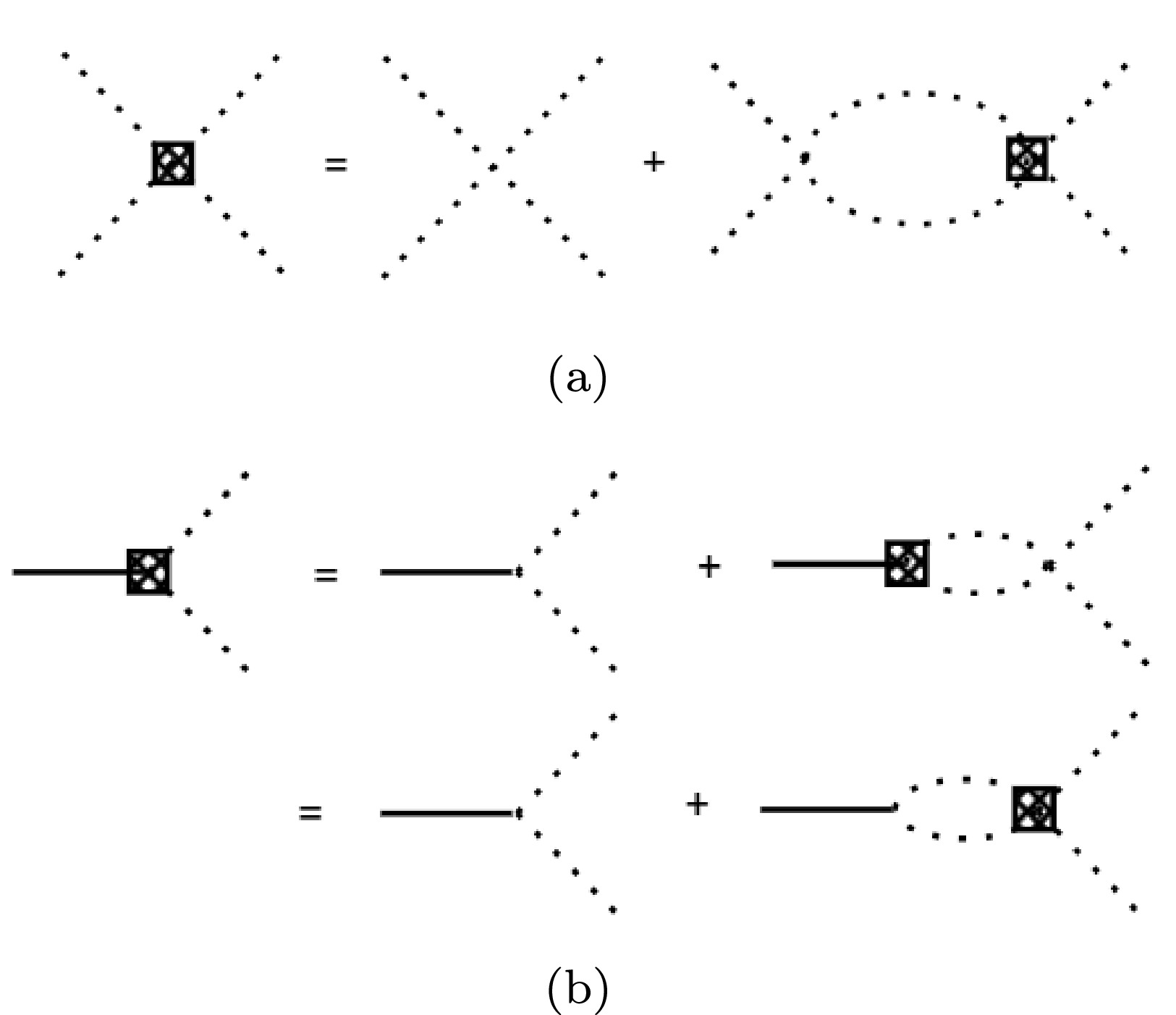

Figure 2.  The LS equation for coupled vertexes. (a) is for $ 2\to2 $ interaction, while (b) is for that of $ 1\to2 $.

The potential $ \tilde{V}^L_{\alpha \beta}\left(k, k^{\prime}, E\right) $ comprises two terms,

where $ V^L_{\alpha \beta}\left(k, k^{\prime}\right) $ is the bare-states-independent potential between two channels(energy-independent on E), while coupling function $ G_{X\alpha} $ describes the coupling between bare state X with bare mass $ m_X $ and channel α. Please note that the spins of these X should be equal to L. The potential $ V^L_{\alpha \beta}\left(k, k^{\prime}\right) $ typically includes t- and u-channel exchanges as well as the contact term. However, for interpolating the scattering data in the finite energy region, separable potential form is a reasonable way to parameterize this potential. Furthermore, such separable potential will promise an exact analytical solution of LS equation, thus, we choose the form of $ v_{\alpha \beta}\left(k, k^{\prime}\right) $ as follows,

where Λ is the QCD energy cut around 1 GeV, $ m_0 $ is the representative meson mass and usually chooses $ m_{\pi_0} $, and $ v^L_{\alpha\beta} $ taken as a real number indicates the coupling constant between channel α and β in the partial wave L The vertex of the bare state X and channel α, $ G^L_{X\alpha}(k) $ can be expressed as,

where $ g^L_{\alpha X} $ is a real dimensionless coupling strength constant.

Based on Eq. (8), the solution of LS equation as shown in Eq. (7) is the T-matrix, $ \tilde{T}^L $, which could be decomposed into two components as follows,

These two parts $ t^L $ and $ T^L $ indicate the contribution from the channels without and with the bare states with the same orbital angular moments L and the same matrix elements$ \alpha\beta $, respectively.

$ t^L $ is defined as

Adopting the separable potential $ {V}^L_{\alpha \beta} $ as shown in Eq. (9), the solution of $ t^{L}_{\alpha \beta} $ inherits a similar separable form as follows,

where

Here, I is unit matrix, the elements of matrix $ v^L $ is $ v_{\alpha\beta} $, and diagonal matrix $ M(E) $ is defined as follows,

The second term at the right side of Eq. (12), $ T^L $, is derived as

where $ {\cal{G}}^L_{\alpha X } $ and $ {\cal{G}}^L_{Y\beta} $ are the dressed coupling functions of $ X\to \alpha $ and $ \beta \to Y $, respectively, and $ A_{XY} $ is the dressed propagator between the bare state X and Y. The two dressed coupling functions can be derived as,

with,

On the other hand, the T-matrix of $ 1\to 2 $ is indeed $ {\cal{G}}^L_{X\alpha}\left(k; E\right) $. The dressed propagator of the bare states is a matrix and elements of its inverse matrix can be expressed as follows

where,

is for the self energy of

The corresponding diagram is shown in Fig. 3.

Figure 3.  The self-energy corrections for propagator.

Finally, we consider the rescattering between $ \bar{X} $ and a. As discussed in the previous subsection, the $ \bar{X} $ can decay, implying this scattering process inherently involves the effect of three-body unitary, which is beyond current model. As shown in Fig. 4, the two right diagrams in the first line show the three-body contribution, the intermediate state could be three states described by dashed lines. Then, we make the assumption that we use a contact term to describe the interaction between $ \bar{X} $ and a, illustrated by the first diagram in the second line. For the triangle loop, we directly absorb it into the width of $ \bar{X} $, which is indicated by the solid triangle in the right diagram in the second line of Fig. 4. Then the energy term of $ \bar{X} $ is replaced as a complex energy $ E-i\ \Gamma/2 $, where Γ denotes the width. Consequently, analogous to the solution of the LS equation mentioned earlier without the bare state contribution, as shown in Eq. (12), with the same separable potential form, we can obtain,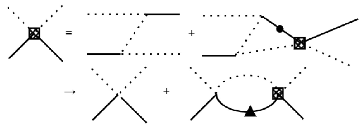

Figure 4.  The diagrams of the scattering between $ \bar{X} $ and a. The Z diagram and triangle loop are proximate to the contact term and two particles loop with a fitted parameter of width of $ \bar{X} $.

where $ \bar{v} $ is the coupling constant matrix.

In the preceding subsection, we have obtained the propagators and coupling vertices involved in the four mechanisms of Fig. 1. The dynamical component of the scattering amplitude directly is an explicit product of these factors, so it remains only to introduce the angular distribution components to obtain the complete partial wave amplitude. Here, we incorporate the partial wave amplitudes to account for the angular distributions. For the background terms and the two processes involving the $ ab $ scattering, we need to consider two angular momentum degrees of freedom, while for the $ \bar{X}a $ process, three degrees of freedom must be taken into account. Consequently, the four reaction amplitudes including the orbital angular momentum can be expressed for an output channel(α) and photon (γ) as:

Here, the three related momenta are all the back-to-back moments in their CMS frame, where dynamic factors like $ f^L $,$ t^L $,$ M^L $,$ A^L $,$ {\cal{G}}^L $ are defined in the last subsection. The spherical harmonics terms $ Y_{LL^z} $ with Clebsch-Gordan coefficients are involved to describe the angular moment contributions for the partial wave amplitudes.

The $ u^{L_1L_2S}_{J/\psi \to \gamma \alpha(X)} $ refers to the coupling strength constants of their subscript processes, where $ L_1 $, $ L_2 $ and S are the angular momentum between γ and $ \alpha(X) $, the total spin of α channel (or the spin of X) and the total spin of $ \gamma \alpha(X) $, respectively. Here, we do not make a detailed expansion since the relative partial-wave amplitudes are written explicitly in Ref. [18]. To clarify the notation, we give an example for X with $ J^{P}=0^{-} $. In this case, only one partial wave survives, $ L_1=1 $, $ L_2=0 $ and $ S=1 $ the formula write as:

where $ \tilde{t}^{(1)\alpha} $ is the p-wave vertex of the γ and X as defined in Ref. [18].

Recognizing the importance and relevance of the comparison between our Lippmann-Schwinger (LS) formalism and the K-matrix, as well as other approaches, we will make a detailed discussion in this subsection.

Firstly, as we point out in the introduction part, the K-matrix method neglects energy-dependent of the real partof self-energy, how it can be modified by introducing $ K=(1-VG^\prime)V $, where $ G^\prime $ is the Chew-Mandelstam variable and V is a potential. However, even though such method still have a significant limitation. It is that the potentials V or K remain independent of the loop integration. This implies an on-shell approximation is applied to both V and K. While this framework may provide adequate data fitting, its predictive capabilities can be questionable.

In our method, we definitely include the off-shell contribution of potential in the loop integration. As shown in Eq. (16), the M matrix replaces the pure two points loop integration in the K-matrix method combining with Chew-Mandelstam variables or the $ i\rho $ term in the pure K-matrix method. In M matrix, it incorporates form factor details from the potential, which indicates the off-shell contribution is reasonably included. Furthermore, this potential is established through theoretical interpolation, with various parameters tightly constrained by symmetries like chiral Lagrangians or SU(3) symmetry. Accordingly, during data fitting, these parameters benefit from robust theoretical constraint.

Conducting a numerical comparison involves inherent challenges, primarily due to the need for identical potentials when comparing the LS approach with the K-matrix approach, or using both to fit similar datasets to evaluate pole positions. Previous work [19] has explored the prediction of the $ P_c $ state, offering detailed comparisons between our LS approach and the Valenca method, a variant of the K-matrix+Chew-Mandelstam approach. Using identical potentials, these calculations yielded differing predictions for the mass of the $ P_c $ state. Notably, the LS approach predicted a smaller binding energy, more closely aligning with experimental measurements at LHCb latter. As such, we do not repeat these calculations here. Latter we will employ a toy model to illustrate the impact of coupled channel contributions.

At last, let us make a discussion about the relativistic Corrections. Relativistic corrections encompass two primary components: kinematic alterations and particle-antiparticle generation from vacuum states. Our methodology incorporates the first through a relativistic dispersion relation. However, the second—which is often overlooked at the hadronic level—remains unsolved in the context of the four-dimensional Bethe-Salpeter equation. The LS approach effectively employs a three-dimensional reduction. This reduction remains justified at the hadronic level; for example, the pion, as the lightest hadron, has a mass approximating 100 MeV, permitting the neglect of antiparticle contributions during propagation. Nevertheless, if current quark structures constitute the foundation of the theory, these relativistic corrections become more pronounced. Presently, such a non-relativistic approach is prevalently adopted in hadronic physics.

This section provides a comprehensive discourse on the comparative strengths and limitations of the various methodologies, highlighting our advancements and situating them within existing theoretical frameworks.

To demonstrate the significance of the coupled-channel effect, we apply our framework to the decay $ J/\psi \rightarrow \gamma K_{S}K_{S} $. In this toy model, we include two pseudoscalar coupled channels($ K_{S}K_{S} $ and $ \pi_0\pi_0 $, with bare masses aset to their PDG values [1]), along with two bare states ($ J^{PC}=0^{+} $): an $ f_0 $ with a bare mass of 1.221 GeV and an $ f^{'}_0 $ at 1.451 GeV. In addition, we include a $ K_1 $ state($ J^{PC}=1^{+} $) with a mass of 1.403 GeV and a width of 0.174 GeV for the $ \gamma K_{S} $ channel. For simplicity, we restrict our analysis to S-wave partial wave amplitudes. The model parameters are listed in Tables 1 and 2.

R {L}	f0 {0}	f0′ {1}
$ m_R $	1.221	1.457
$ g_{(R,KK)} $	0.810	−0.710
$ g_{(R,\pi\pi)} $	−0.740	0.910
$ u_{(J/\psi,\gamma R)} $	0.300	0.500
$ \gamma PP$
$ v_{KK,KK} $	0.980	−
$ v_{KK,\pi\pi} $	0.870	−
$ v_{\pi\pi,\pi\pi} $	0.980	−
$ u_{(J/\psi,\gamma KK)} $	0.800	−
$ u_{(J/\psi,\gamma \pi\pi)} $	0.800	−

Table 1.  Parameters for the Considered Dual-Channel Decay PP Model. The meaning of each parameter is defined in the description provided in the previous section. All energy units are GeV, and the QCD energy cutoffs Λ are fixed at 1 GeV.

R {L}	K1 {0}
$ m_R $	1.403	−
$ \Gamma_R $	0.174	−
$ \bar{u}_{(J/\psi,KR)} $	1.400	−
$ \bar{v}_{(KR,KR)} $	1.000	−
$ \bar{g}_{(R,\gamma K)} $	1.000	−

Table 2.  Parameters for the Considered Dual-Channel Decay XP Model. See Tables I for the description.

We first determine the pole positions of the T-matrix in the complex energy plane for the two-pseudoscalar coupled channels by solving $ \ Det[A_{XY}(E)^{-1}]=0 $ on the relevant Riemann sheets. For the $ ab $ coupled channels, we identify two pole positions in the second Riemann sheets(denoted as $ uu $), as summarized in Table 3. For the $ K_1K_{S} $ channel, the width in the $ K_1 $'s propagator is pre-set, and its pole position is fixed to $ M_{poles}=m_{bare}-i \Gamma/2 $. While the real and imaginary parts of the pole position in a unitary model generally differ from the BW mass and width, they converge for narrow resonances [20]. Our model shows that the two $ f_0 $ resonances, generated via the bare-state couplings, exhibit narrow widths, resulting in invariant mass peaks consistent with their pole positions. In contrast, the broader $ K_1 $ resonance($ \Gamma\approx $150 MeV) undergoes significant lineshape modifications due to $ K_1K_{S}\to K_1K_{S} $ rescattering, leading to an observable shift in the $ \gamma K_{S} $ invariant mass spectrum.

R{L}	$ M_{pole} $(GeV)	$ {\rm{RS}} $
$ f_0\{0\} $	$ 1.225-0.010\ i $	$ (uu) $
$ f^{'}_0\{0\} $	$ 1.457-0.007\ i $	$ (uu) $
$ K_1\{0\} $	$ 1.403-0.087\ i $	−

Table 3.  Pole positions in PP scattering case amplitudes. The Riemann sheets of them are specified by ($ KK,\pi\pi $). for the $ K_1 $ resonance, we take its pole position from the BW form. The real part is very close to the input mass of $ K_1 $, and the imagery part is obtain by $ Im(M_{pole})=-\Gamma(Res)/2 $.

We now present the Daliz plots for the reaction. The distributions of the sum of Fig. 1(a-c), pure Fig. 1(d) and the full amplitudes are shown in Fig. 5(a-c), respectively. Two clear $ f_0 $ signals presented as red lines in Fig. 5(a), and one signal for $ K_1 $ as shown blue broad belt in Fig. 5(b) emerge, corresponding to the intermediate states in our model. Interference between these components significantly distorts the $ K_1 $ lineshape, underscoring the necessity of including all mechanisms. An enhancement is observed at high $ M_{K_{S}K_{S}} $ and low $ M_{\gamma K_{S}} $, arising from interference between the tree-level diagram and dynamical rescattering effects.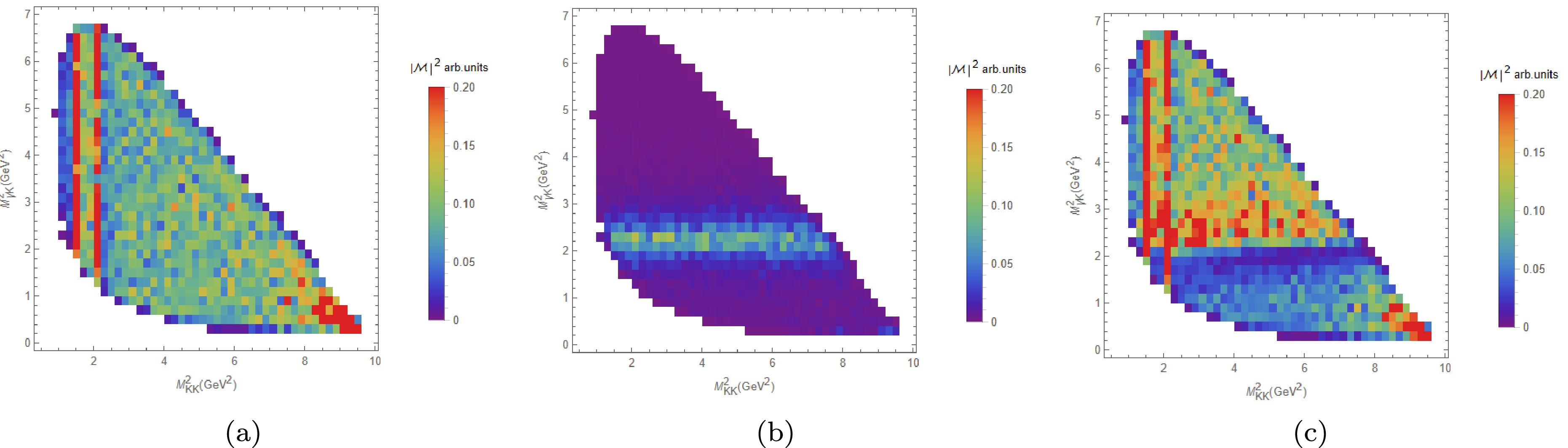

Figure 5.  (color online) The Dalitz plot on $ M^2(K K) $ and $ M^2(\gamma K) $for different amplitudes' square.(a) Tree-level, PP-rescattering and Bare states;(b) XP-rescattering; (c) All amplitudes.

To elucidate the contributions of dynamical mechanisms, Fig. 6 decomposes the contributions of individual mechanisms. We find that the mechanism shown in Fig. 1(c) provides the primary contribution to two $ f_0 $ resonance peaks, while Fig. 1(a)(b) remain essentially flat. However, their interference enhances contributions in the high-energy region of $ M_{K_{S}K_{S}} $ and also strengthens the background under both $ f_0 $ resonance peaks. Thus, the analysis demonstrates the coupled-channel model is crucial for a unified treatment of various background contributions, and the correct description of the background is also extremely important for extracting resonance structures. Regarding the mechanism shown in Fig. 1(d), it does not produce any special structure in the invariant mass spectrum of $ K_{S} K_{S} $, but generates a subtle bump via interference from other channels in the high-energy region. This explains the observed statistical enhance in the high $ M_{K_{S}K_{S}} $ region on the Dalitz plot. Similarly, in the $ \gamma K $ invariant mass spectrum, the $ \bar{X}b $ rescattering as shown in Fig. 1(d) clearly dominates the peak structure, which undergoes a measurable shift due to the interference with contributions of Fig. 1(a-c). These results highlight the critical role of coupled-channel effects in resonance analysis: interference can distort lineshapes from simple BW expectations, necessitating a unified framework for accurate mass/width extraction.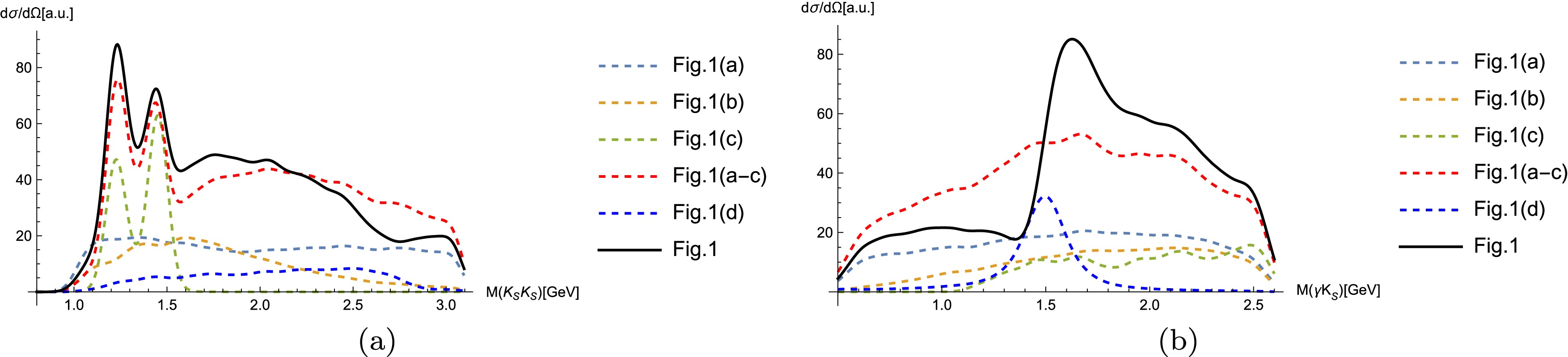

Figure 6.  (color online) One-dimensional projection plot for each amplitudes on $ M(\gamma K) $ and $ M(KK) $ invariant mass spectrum. The lines refers which amplitudes is shown in the legend. (a)$ M(KK) $ invariant mass spectrum; (b)$ M(\gamma K) $ invariant mass spectrum.

In this article, we develop a unitary coupled-channel framework for a system of two pseudoscalar mesons, explicitly distinguishing between resonant signals and non-resonant background contributions. The model is applied to the radiative decay $ J/\psi\to\gamma ab $, incorporating rescattering effects between the final-state mesons. This framework includes the tree-level decay of $ J/\psi $ into the final-state pseudoscalar mesons, the cascade decay of $ J/\psi $ radiating into a resonance particle which subsequently decays into $ ab $, the rescattering process where $ J/\psi $ radiates into $ ab $, followed by final-state interactions, and the chain of $ J/\psi $ decaying into one pseudoscalar meson and an intermediate resonance, which then radiates another pseudoscalar meson via scattering. Additionally, the decay of the $ f_0 $ resonance includes contributions from meson rescattering. In contrast, conventional isobar models typically describe cascade decays through a BW parametrization of intermediate resonances, supplemented with ad hoc background terms. Such approaches often introduce arbitrariness in modeling background structures, leading to uncertainties in resonance parameter extraction. Our coupled-channel formalism, however, is constrained by $ ab $ scattering, providing a self-consistent description of both resonant and non-resonant effects, thereby minimizing model-dependent ambiguities. Despite its computational complexity, this approach offers significant theoretical advantages for practical data analysis.

For the three-body system $ \gamma ab $, considering only $ ab $ coupled-channel effects is insufficient. Although photon-induced electromagnetic interactions are weak (allowing photon-meson rescattering to be neglected), an additional coupled-channel effect arises: the rescattering between a meson $ \bar{X} $ (coupled the $ \gamma a $ system) and another pseudoscalar meson. We derive the corresponding formalism to incorporate this process. Combining these four mechanisms, we establish a comprehensive theoretical framework for $ J/\psi\to\gamma ab $, essential for future experimental analyses of this decay.

To illustrate the framework, we construct a toy model for $ J/\psi \to \gamma K_{S} K_{S} $, introducing two $ f_0 $-resonances and one $ K_1 $ meson. The $ f_0 $-resonances coupled to $ K\bar{K} $, with additional contributions from the $ \pi\pi $ coupled channel, forming a two-bare-state, two-channel system. The $ K_1 $ meson couples to $ \gamma K_{S} $, as described earlier. By evaluating all four mechanisms, we compute the Dalitz plot and invariant mass spectra for $ K_{S}K_{S} $ and $ \gamma K_{S} $. The results demonstrate that the peaks of the $ f_0 $-resonances emerge atop smooth backgrounds, while the $ K_1 $ peak exhibits significant distortion due to interference effects, deviating markedly from its nominal resonance profile. These findings highlight the necessity of a unified treatment of signals and backgrounds for correct experimental interpretation.

This work aims to provide a coupled-channel-based amplitude analysis framework for the analysis of the extremely high-precision data and to advance the study of glueballs by taking into account coupled-channel effects in a self-consistent way.