


 Abstract
 HTML
HTML Reference
 Related
 PDF
PDF


-
The vacuum expectation values of the stress tensor and power spectrum of quantum fields in curved spacetimes have direct observational effects in cosmology. However, these physical quantities are prone to UV divergences [1-3]. To remove UV divergences, several approaches have been proposed for regularization, such as dimensional regularization [4-7], covariant point-splitting [8-14], and the zeta function [5, 15, 16]. These methods involve the Green's function and are essentially equivalent [5]. The appropriate subtraction term to the Green's function in position space is generally hard to determine. Only for the massless scalar field in de Sitter space with conformal or minimal coupling, the subtraction term has been found [17]. Different from the above approaches, adiabatic regularization works with the k-modes [18-32], and by the minimal subtraction rule, the power spectrum is regularized to the 2nd order and the stress tensor to the 4th order. For a massive scalar field with
$ \omega = (k^2+m^2)^{1/2} $ as the 0th-order frequency, this prescription is sufficient in removing all UV divergences, but sometimes removes more than necessary, leading to negative spectra, as demonstrated in de Sitter space [17]. In fact, 0th-order regularization is sufficient to achieve nonnegative UV- and IR-convergent spectra for a massive scalar field with conformal coupling, and, similarly, so is 2nd-order regularization for minimal coupling. Given the regularized power spectrum, the Fourier transformation produces the regularized Green's function, which is UV- and IR-convergent [17].In this paper we extend the study to general spatially flat RW spacetimes. We shall consider a massless scalar field with a coupling
$ \xi $ , whose exact solution is available and regularization can be performed in an analytical manner. Our aim is to search for proper regularization schemes that will yield nonnegative UV- and IR-convergent power spectrum and spectral energy density. As shall be shown, the goal can be eventually achieved, but there is no universal scheme that would work for all couplings and all RW spacetimes. First, UV convergence can be easily achieved by regularization of a certain order. Unlike a massive field, the 0th-order frequency of a massless field is the wavenumber k, so that the 2nd-order regularization for the power spectrum and the 4th order for the spectral stress tensor are necessary to remove all UV divergences. In particular, for the conformal coupling$ \xi = \frac16 $ , the regularization of all orders are equivalent, yielding a zero power spectrum and a zero spectral stress tensor, and there is no trace anomaly. For the minimal coupling$ \xi = 0 $ , the regularized power spectrum and spectral stress tensor are zero in several important RW spacetimes, such as radiation-dominated (RD) expansion, matter-dominated (MD) expansion, and de Sitter space. For general couplings and general RW spacetimes, however, the regularized spectra can be negative, as demonstrated herein. To avoid this negative spectrum, we attempt to increase the order of regularization on the pertinent spectrum as this will generally yield a positive spectrum. Nevertheless, this higher-order regularized, positive spectrum tends to carry new IR divergence, which is characteristic of the adiabatically regularized spectra of a massless field [32]. To retain IR convergence, we shall apply the inside-horizon scheme of regularization, by which the long wavelength modes outside the horizon are fixed and only the short wavelength modes inside the horizon are regularized [32]. Finally, we shall achieve nonnegative UV- and IR-convergent power spectrum and spectral energy density.The paper is organized as follows.
In Sec. 2, we derive the exact solution of a coupling massless scalar field and its Green's function in general RW spacetimes, analyze the behaviors of the power spectrum and the spectral stress tensor, and give the prescriptions of adiabatic regularization.
In Sec. 3, for the conformal coupling
$ \xi = \frac16 $ , we show that adiabatic regularization of various orders are equal, yielding zero power spectrum and zero stress tensor, and there is no trace anomaly in general RW spacetimes. We also present direct regularization of the Green's function, confirming the result of adiabatic regularization.Sec. 4 considers the minimal coupling
$ \xi = 0 $ . We show that the regularized power spectrum and stress tensor are zero in several important RW spacetimes, the results of which are also confirmed by regularization of the Green's functions. In general RW spacetimes, we use two examples to show that regularized spectra can be negative, and the pertinent spectrum will become positive by realizing higher-order regularization, thereby also acquiring IR divergence. The IR divergence will be avoided by the inside-horizon scheme.Sec. 5 presents the case for the general coupling
$ \xi $ , the analysis of which is similar to that in Sec. 4.Sec. 6 provides the conclusion and discussions.
Appendix A lists high-k expansions of the exact modes. Appendix B lists the WKB solutions and the associated subtraction terms up to the 6th order, and demonstrates the covariant conservation to each adiabatic order.
-
In a flat Robertson-Walker spacetime
$ {\rm d}s^2 = a^2(\tau)[{\rm d}\tau^2- \delta_{ij} {\rm d}x^i{\rm d}x^j], $

(1) with the conformal time
$ \tau $ , a massless scalar field has the Lagrangian density$ {\cal L} = \frac12 \sqrt{-g} \left( g^{\mu\nu}\phi_{,\mu}\phi_{,\nu} -\xi R\phi^2 \right) , $

(2) and the field equation [2, 13, 25]
$ \left( \Box + \xi R \right)\phi = 0 , $

(3) where
$ \Box = \frac{1}{a^4} \frac{\partial}{\partial \tau} (a^2 \frac{\partial}{\partial \tau}) -\frac{1}{a^2} \nabla^2 $ ,$ R = 6 a''/a^{3} $ is the scalar curvature,$ \xi $ is the coupling constant, and we consider a range$ 0 \leqslant \xi \leqslant \frac16 $ specifically; and$ \phi ({{{x}}},\tau) = \int\frac{{\rm d}^3k}{(2\pi)^{3/2}} \left[ a _{{{{k}}}} \phi_k(\tau) {\rm e}^{{\rm i}{{k}}\cdot{{x}}} +a^{\dagger}_{{{{k}}}} \phi^{*}_k(\tau) {\rm e}^{-{\rm i}{{k}}\cdot{{x}}}\right], $

where
$a_{{{{k}}}}, a^{\dagger}_{{{{k}}}}$ are the annihilation and creation operators, respectively, that satisfy the canonical commutation relation, and$ \phi_k(\tau) $ is the k-mode, written as$ \phi_k(\tau) = v_k(\tau)/a(\tau) $ . The equation of the rescaled$ v_k $ mode is$ v_k'' + \Big( k^2 + \Big(\xi -\frac16 \Big) a^2 R \Big) v_k = 0 . $

(4) In this paper we consider a class of power-law expanding RW spacetimes,
$ a(\tau) = a_0 |\tau|^{b} , $

(5) where the expansion index b is a constant,
$ a^2 R = 6 b(b- 1) \tau^{-2 } $ . The positive-frequency mode solution of (4) is$ v_k (\tau ) \equiv \sqrt{\frac{\pi}{2}}\sqrt{\frac{x}{2k}} {\rm e}^{{\rm i} \frac{\pi}{2}(\nu+ \frac12) } H^{(1)}_{\nu} ( x) , $

(6) where
$ x \equiv k |\tau| $ ,$ H^{(1)}_{\nu} $ are the Hankel functions, and$ \nu \equiv \sqrt{\frac14 -( 6\xi -1) b(b-1)} . $

(7) Three cases lead to a special value
$ \nu = \frac12 $ : the conformal coupling ($ \xi = \frac16 $ ), the Minkowski spacetime ($ b = 0 $ ), and the RD expansion ($ b = 1 $ ), and in these cases mode (6) reduces to$ v_k (\tau ) = i \sqrt{\frac{\pi}{2}}\sqrt{\frac{x}{2k}} H^{(1)}_{\frac12} ( x) = \frac{1}{\sqrt{2k} } {\rm e}^{-{\rm i} k\tau} , $

(8) conformal to the mode in Minkowski spacetime. Mode (6) of a general
$ \nu $ at high k also approaches (8).The Bunch-Davies vacuum state is defined such that
$ a_{{{{k}}}} |0 \rangle = 0, \; \; \; {\rm{for}}\; {\rm{all}} \ {{{{k}}}} . $

(9) In a general RW spacetime the unregularized Green's function in the vacuum is
$ \begin{split} G(x^{\mu}, x'\, ^{\mu}) &= \langle0| \phi({{{r}}},\tau) \phi ({{{r}}}',\tau') |0\rangle = \frac{1}{(2\pi)^3} \int {\rm d}^3k \, {\rm e}^{{\rm i} {{{k}}} \cdot ({{r}}-{{r}}')} \phi_k(\tau) \phi_{k}^* (\tau ') \\ & = \frac{1}{ a(\tau)a(\tau')} \frac{|\tau|^{1/2} |\tau'|^{1/2} }{8 \pi } \int_0^\infty {\rm d} k k \frac{\sin( k|r-r'|)}{ |r-r'| } H^{(1)}_{\nu} (k\tau ) H^{(2)}_{\nu} (k\tau') . \end{split} $

(10) The integration in (10) can be carried out [13, 17, 33], and the result is a hypergeometric function, as follows
$\begin{split} G(\sigma) =& \frac{1}{16 \pi^2 a(\tau)a(\tau') |\tau \tau'| } \Gamma \Big( \frac{3}{2}-\nu \Big) \Gamma \Big( \nu +\frac{3}{2} \Big) \, \\&\times _2F_1\left[\frac{3}{2}+\nu ,\frac{3}{2}-\nu ,2, \; 1 + \frac{\sigma}{2} \right] \, , \end{split}$

(11) where
$ \sigma = [(\tau-\tau')^2-(r-r')^2 ]/(2 \tau \tau') $ is half of the squared geometric distance between two points$ x^{\mu} $ and$ x'^{\mu} $ . For the equal-time$ \tau = \tau' $ case the Green's function is$\begin{split} G({{{r}}}- {{{r}}}') =& \langle0| \phi({{{r}}},\tau) \phi ({{{r}}}',\tau) |0\rangle \\=& \int_0^\infty \frac{\sin( k|r-r'|)}{|r-r'|\, k^2} \Delta^2_k (\tau) \, {\rm d} k , \end{split}$

(12) the auto-correlation function is
$\begin{split} G(0) =& \langle0| \phi({{r}},\tau) \phi ({{r}},\tau) |0\rangle = \frac{1}{(2\pi)^3} \int {\rm d}^3k \, |\phi_k(\tau)|^2\\ =& \int_0^{\infty}\Delta_k^2 (\tau)\frac{{\rm d}k}{k} , \end{split}$

(13) and the power spectrum is
$ \Delta_k^2 (\tau) = \frac{ k^{3}}{2 \pi^2 a^2 (\tau) } |v_k(\tau)|^2 = \frac{ x^{3} }{8 \pi a^2(\tau)\tau^{2} } | H^{(1)}_{\nu} ( x)|^2 . $

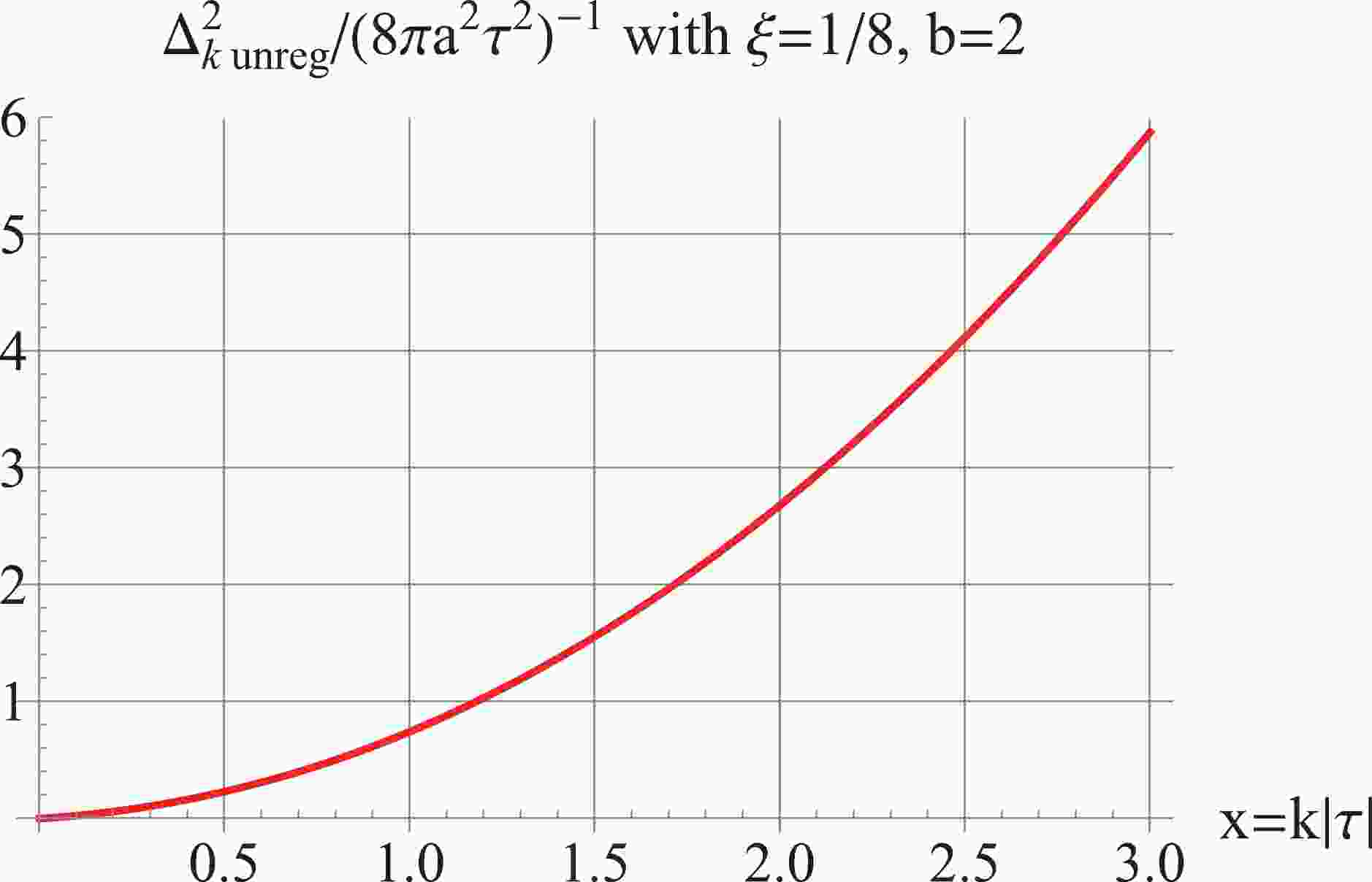
(14) The power spectrum is shown in Fig. 1 for
$ b = 2 $ and$ \xi = \frac18 $ , which is UV-divergent, leading to an infinite auto-correlation$ G(0) $ . This also indicates that the stress tensor in (23) as well as the trace in (24) will generally be divergent as they contain a term$ \propto \phi^2 $ . The asymptotic behaviors of the power spectrum can be analyzed by series expa-nsion. At high k, the power spectrum for general$ \xi $ and b is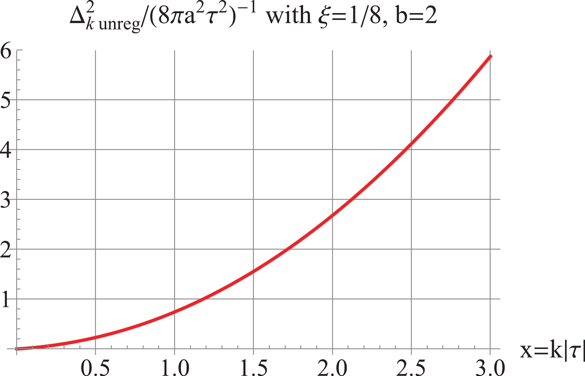
Figure 1. (color online) The unregularized
$ \Delta^2_k $ for$ b = 2 $ and$ \xi = \frac18 $ . The plot is with$ |\tau| = 1 $ for illustration.$ \begin{split} \Delta _k^2(\tau ) =& \frac{1}{{4{\pi ^2}{a^2}{\tau ^2}}} \bigg[{x^2} - \frac{{(6\xi - 1)(b - 1)b}}{2} - \frac{{3(6\xi - 1)(b - 1)b\left[ {(1 - 6\xi )({b^2} - b) - 2} \right]}}{{8{x^2}}}\\ &- \frac{{5(6\xi - 1)(b - 1)b\left[ {(1 - 6\xi )({b^2} - b) - 2} \right]\left[ {(1 - 6\xi )({b^2} - b) - 6} \right]}}{{16{x^4}}} + ...\bigg]. \end{split} $

(15) The first two terms are quadratic and logarithmic UV-divergent. Our task is to perform adiabatic regularization and establish a power spectrum that should be: 1) UV-convergent, 2) IR-convergent, 3) nonnegative. By the minimal subtraction rule [29], the first two terms of (15) are subtracted off under the 2nd-order regularization,
$ \Delta^2_{k\,\rm reg} = \frac{ k^{3}}{2 \pi^2 a^2 } \Big( |v_k(\tau)|^2 -|v_k^{(2)}(\tau)|^2 \Big), $

(16) where
$ |v_k^{(2)}(\tau)|^2 $ is the subtraction term given by (B13), formed from the 2nd-order WKB approximate solution. The 2nd-order regularized power spectrum (16) is UV-convergent; however, it can be negative for certain values of$ \xi $ and b, as can be checked by the dominant third term of Eq. (15),$ -\frac{3(6 \xi -1) (b-1) b \left[(1-6\xi ) (b^2-b)-2\right]}{8 x^2} $

(17) at high k. When this term is negative, to obtain a positive power spectrum, we shall try the 4th-order regularized power spectrum,
$ \Delta^2_{k\,\rm reg} = \frac{ k^{3}}{2 \pi^2 a^2 } \Big( |v_k(\tau)|^2 -|v_k^{(4)}(\tau)|^2 \Big), $

(18) where
$ |v_k^{(4)}(\tau)|^2 $ is given by (B21), constructed from the 4th-order WKB approximate solution, and removes the first three terms of Eq. (15). This usually yields a positive, UV-convergent power spectrum, which is dominated at high k by the fourth term of Eq. (15)$ -\frac{5(6 \xi -1)(b-1) b\left[(1-6\xi ) (b^2-b)-2\right] \left[ (1-6\xi ) (b^2-b)-6\right] }{16 x^4} . $

(19) We have checked that (19) is positive when (17) is negative. We shall demonstrate this procedure using examples in later sections.
We examine the low-k behavior of
$ \Delta^2_{k} $ . For$ \xi = \frac{1}{6} $ , or$ b = 1 $ , it has only one term,$ \Delta^2_{k} = \frac{ k^{3}}{2 \pi^2 a^2} \frac{1}{2 k} , $

(20) which also holds for all k. For a general
$ \xi $ by (A6), it is$ \Delta_k^2 (\tau) \simeq \frac{2^{2\nu}}{8 \pi^3 a^2 \tau^{2}} \Gamma(\nu)^2 x^{3-2\nu } \propto k^{3-2\nu }. $

(21) Regarding inflationary cosmology, if the scalar field
$ \phi $ is used to model the perturbed inflaton scalar field during inflation, the power spectrum$ \Delta_k^2 $ at low k realizes the primordial spectrum of scalar field perturbations, which is often written in the form of$ \Delta_k^2 \propto k^{\, n_s -1} . $

Thus, one reads off the scalar spectral index
$ n_s = 4-2\nu = 4- 2 \sqrt{\frac14 -( 6\xi -1) b(b-1)}\; . $

(22) The currently observed value is
$ n_s\simeq 0.96 $ , which for$ \xi = 0 $ corresponds to an expansion index$ b\simeq -1.02 $ during inflation [31, 32]. In general RW spacetimes, the power spectrum (21) with$ \xi = 0 $ is IR-convergent for$ -1<b<2 $ , and is IR-divergent for$ b \leqslant -1 $ or$ b \geqslant 2 $ . In this paper, we do not discuss the issue of IR divergence in the unregularized power spectrum, which can be avoided either by a certain initial condition or by some precedent expansion stage, as has been studied in Refs. [34, 35]. Nevertheless, for a massless field, sometimes regularization may transform an IR-convergent power spectrum into IR-divergent. This is a matter of concern within this paper. When this transformation occurs, to retain the IR convergence, we can adopt the scheme of inside-horizon regularization, i.e, the long wavelength modes outside the horizon are fixed and only the short wavelength modes inside the horizon are regularized [32]. By this procedure, the regularized power spectrum will remain IR-convergent.The stress tensor plays the role of a source of gravity in general relativity. For the massless scalar field, it is given by [25, 26]
$ \begin{split} T_{\mu\nu} =& (1-2\xi) \partial_ \mu \phi \partial_ \nu \phi +\left(2\xi - \frac12\right) g_{\mu\nu } \partial^\sigma \phi \partial_\sigma \phi -2\xi \phi_{;\mu\nu} \phi \\ & + \frac12 \xi g_{\mu\nu} \phi \Box \phi -\xi \left(R_{\mu\nu}-\frac12 g_{\mu\nu} R + \frac32 \xi R g_{\mu\nu}\right) \phi^2, \end{split} $

(23) which satisfies the covariant conservation
$ T^{\mu\nu}_{\; \; \; ;\nu} = 0 $ by virtue of field equation (3). The trace is$ T^{\mu}\, _\mu = (6\xi -1) \partial^ \mu \phi \partial_ \mu \phi +\xi (1-6\xi) R \phi^2 . $

(24) The energy density in the BD vacuum state is given by the expectation value
$ \rho = \langle T^0\, _0 \rangle = \int^{\infty}_0 \rho_k \frac{{\rm d} k}{k} , $

(25) where the spectral energy density is
$\begin{split} \rho_k =& \frac{ k^3}{4\pi^2 a^4} \Big[ |v_k'|^2 + k^2 |v_k|^2 + (6\xi-1) \\&\times\Big( \frac{a'}{a} (v'_k v^*_k + v_k v^*_k ' ) - \Big(\frac{a'}{a}\Big)^2 |v_k|^2 \Big) \Big] ,\end{split} $

(26) the trace of the stress tensor is
$ \begin{split} \langle T^{\mu}\, _\mu \rangle =& \frac{1}{2\pi^2 a^4} \int k^2 {\rm d}k \, (6\xi-1)\times\Big [ |v_k'|^2 - \frac{a'}{a} (v'_k v^*_k + v_k v^*_k ' ) \\ &- k^2 |v_k|^2 -\Big(\frac{a''}{a} - \Big(\frac{a'}{a}\Big)^2 \Big) |v_k|^2 + (1- 6\xi) \frac{a''}{a} |v_k|^2 \Big] , \end{split} $

(27) the pressure is
$ p = -\frac13 \langle T^i \, _i \rangle = \int^\infty_0 p_k \frac{{\rm d}k}{k} , $

(28) where the spectral pressure is
$ \begin{split} p_k =& \frac{k^3}{4 \pi^2 a^4} \Big[ \frac13 |v_k'|^2 + \frac13 k^2 |v_k|^2 + 2\Big(\xi-\frac16\Big)\\&\times\Big( \frac{a'}{a} (v'_k v^*_k + v_k v^*_k ' ) - (\frac{a'}{a})^2 |v_k|^2 \Big) \\& - 4\Big(\xi-\frac16\Big)\Big( |v_k'|^2 - \frac{a'}{a} (v'_k v^*_k + v_k v^*_k ') - k^2 |v_k|^2 \\&- \Big(\frac{a''}{a} -\Big (\frac{a'}{a}\Big)^2\Big) |v_k|^2 - 6\Big(\xi-\frac16\Big) \frac{a''}{a} |v_k|^2 \Big)\Big] . \end{split} $

(29) For each k-mode, the unregularized spectral stress tensor satisfies the covariant conservation
$ \rho_{k }' + 3 \frac{a'}{a} (\rho_{k} + p_{k}) = 0 $ , as can be checked by field equation (4). The spectral energy density and pressure have the following high-k expansions$ \begin{split} \rho_k =& \frac{1}{4\pi^2 a^4\tau^4}\left[ x^4 -\frac{(6 \xi-1)b^2 x^2}{2 }+\frac{3 (6 \xi -1)^2(b-1)b^2 (b+1) }{8} +\frac{5(6 \xi -1)^2 (b-1) b^2 (b+2)\left[(1- 6\xi) (b^2-b)-2\right] }{16 x^2} \right.\\ &\left. +\frac{35 (6 \xi -1)^2b^2 (b-1) (b+3) [b (b-1) (6 \xi -1)+2 ] [(b-1) b (6 \xi -1)+6 ]}{128 x^4} + ...\right] , \end{split} $

(30) $ \begin{split} p_k =& \frac{1}{4 \pi^2 a^4\tau^4} \left[ \frac{x^4}{3} -\frac{(6 \xi -1)b (b+2) x^2}{6} +\frac{ (6 \xi -1)^2(b-1)b(b+1) (b+4)}{8} + \frac{5(6 \xi -1)^2(b-1) b(b+2) (b+6) \left[(1- 6\xi) (b^2-b)-2\right]}{48 x^2} \right.\\ &\left. + \frac{35 \;(6 \xi -1)^2 (b-1) b (b+3) (b+8) [ (b-1) b (6 \xi -1)+2] [(b-1) b (6 \xi -1)+6]}{384 x^4} +... \right] , \end{split} $

(31) both containing quartic, quadratic, and logarithmic UV divergences. The quartic divergences come from the derivative terms, such as
$ \partial_ \mu \phi \partial_ \nu \phi $ , except$ \phi^2 $ . Thus, we search for a regularized stress tensor that should satisfy the following criteria: 1) UV-convergent, 2) IR-convergent, 3) nonnegative spectral energy density. A negative pressure is allowed, so we focus on the spectral energy density in this paper. By the minimal subtraction rule [18], the first three divergent terms of$ \rho_k $ in (30) are subtracted off under the 4th-order regularization,$ \rho_{k\,\rm reg} = \rho_{k} - \rho_{k\, A 4 } , $

(32) where
$ \rho_{k\, A 4} $ is the 4th-order subtraction term given by (B37). The resulting$\rho_{k\,\rm reg}$ is always UV-convergent, and if it is also positive, our goal has been achieved. Like the power spectrum, however, the 4th-order regularized$ \rho_k $ can be negative for certain values of$ \xi $ and b, as is determined using the dominant fourth term of Eq. (30) at high k,$ \frac{5(6 \xi -1)^2 (b-1) b^2 (b+2) \Big((1- 6\xi) (b^2-b)-2 \Big) }{16 x^2} . $

(33) When this happens, to obtain a positive spectral energy density, we try the 6th-order regularization
$ \rho_{k\,\rm reg} = \rho_{k} - \rho_{k\, A 6 } , $

(34) where the subtraction term
$ \rho_{k\, A 6} $ is given by Eq. (B39). Under this subtraction, the first four terms of (30) will be removed, and the fifth term$ \frac{35 (6 \xi \!\!-\!\!1)^2b^2 (b\!\!-\!\!1) (b\!\!+\!\!3) \Big(b (b\!\!-\!\!1) (6 \xi \!\!-\!\!1)\!\!+\!\!2 \Big) \Big((b\!\!-\!\!1) b (6 \xi \!\!-\!\!1)\!\!+\!\!6 \Big) }{128 x^4} $

(35) remains and dominates the 6th-order regularized spectral energy density at high k. As will be demonstrated, for the RW spacetimes used in cosmology, this often gives a positive, UV-convergent regularized spectral energy density. For those rarely used in cosmology, say
$ -3<b<-2 $ , and for a coupling$ \frac{b^2-b-2}{6 b^2-6 b}<\xi <\frac{1}{6}, $

(36) both Eqs. (33) and (35) will be negative for high k. Then, the 8th-order regularized
$ \rho_k $ must be determined, which is dominated by the following term$ \begin{split}& \frac{1}{4\pi^2 a^4\tau^4}\Big[ -\frac{1}{256 x^6}63 (b-1) (b+4) b^2(1-6 \xi )^2 \Big((b-1) b (6 \xi -1) \\&\quad+2\Big) \Big((b-1) b (6 \xi -1) +6\Big) \Big((b-1) b (6 \xi -1)+12\Big) \Big] .\\[-16pt] \end{split} $

(37) This term is positive with a coupling in the range of (36). Thus, a positive UV-convergent spectral energy density can be achieved using this procedure.
We mention that the four-divergence of the subtraction terms to the stress tensor is zero under regularization of each order, so that the covariant conservation is respected by the regularized stress tensor respects (See (B45)–(B50) in Appendix B).
We examine the low-k behavior of the stress tensor. For
$ \xi = \frac16 $ , or$ b = 1 $ , Eq. (7) gives$ \nu = \frac12 $ , and (26) and (29) reduce to$ \rho_k = \frac{ k^3}{4\pi^2 a^4} \Big[ |v_k'|^2 + k^2 |v_k|^2 \Big] = \frac{ k^3}{4\pi^2 a^4} k , \; \; \; \; p_k = \frac13 \rho_k , $

(38) which are UV-divergent and IR-convergent. For
$ \xi = 0 $ , (26) and (29) reduce to$ \rho_k = \frac{ k^3}{4\pi^2 a^2} \Big[ \Big|\Big(\frac{v_k}{a}\Big)' \Big|^2 + k^2 \Big|\frac{v_k}{a} \Big|^2 \Big] , $

(39) $ p_k = \frac{k^3}{4 \pi^2 a^2} \Big[ \Big|\Big(\frac{v_k}{a}\Big)' \Big|^2 - \frac13 k^2 \Big|\frac{v_k}{a}\Big|^2 \Big] , $

(40) shown in Fig. 2, while at low k they reduce to
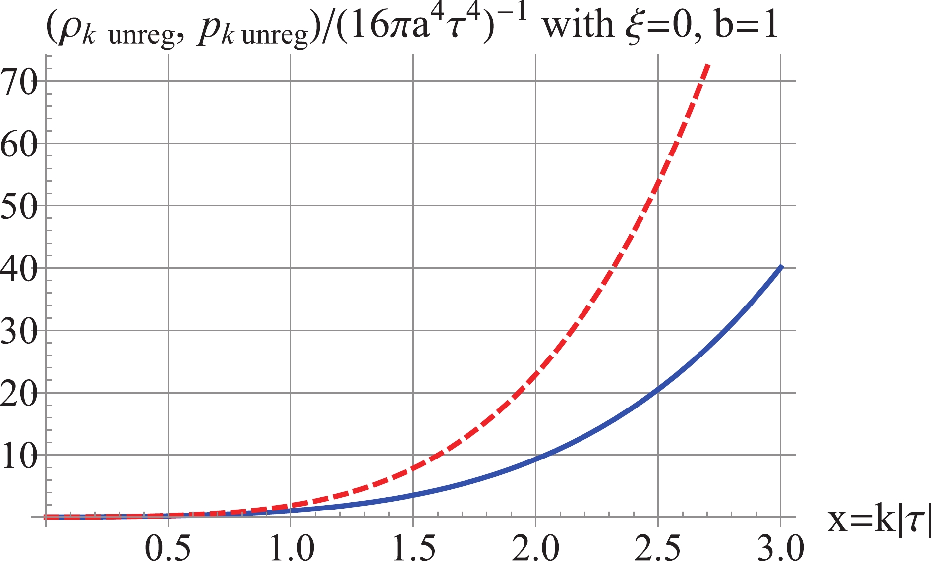
Figure 2. (color online) Red Dash: unregularized
$ \rho_k $ , Blue Solid: unregularized$ p_k $ . For$ \xi = 0 $ and$ b = 1 $ .$ {\rho _k} \simeq \left\{ {\begin{array}{*{20}{l}} {\dfrac{{{2^{2 + 2\nu }}}}{{16{\pi ^3}{a^4}{\tau ^4}}}\Gamma {{(\nu + 1)}^2}{x^{3 - 2\nu }},}&{b \geqslant \dfrac{1}{2},}\\ {\dfrac{{{2^{2 - 2\nu }}}}{{16\pi {a^4}{\tau ^4}}}\dfrac{{{x^{2\nu + 3}}}}{{{{\sin }^2}(\pi \nu )\Gamma {{(\nu )}^2}}},}&{0 < b < \dfrac{1}{2},}\\ {\dfrac{{{x^4}}}{{4{\pi ^2}{a^4}{\tau ^4}}},}&{b = 0,}\\ {\dfrac{{{2^{2\nu }}}}{{16{\pi ^3}{a^4}{\tau ^4}}}\Gamma {{(\nu )}^2}{x^{5 - 2\nu }},}&{b < 0,} \end{array}} \right. $

(41) $ {p_k} \simeq \left\{ {\begin{array}{*{20}{l}} {\dfrac{{{2^{2 + 2\nu }}}}{{16{\pi ^3}{a^4}{\tau ^4}}}\Gamma {{(\nu + 1)}^2}{x^{3 - 2\nu }},}&{b \geqslant \dfrac{1}{2},}\\ {\dfrac{{{2^{2 - 2\nu }}}}{{16\pi {a^4}{\tau ^4}}}\dfrac{{{x^{2\nu + 3}}}}{{{{\sin }^2}(\pi \nu )\Gamma {{(\nu )}^2}}},}&{0 < b < \frac{1}{2},}\\ {\dfrac{{{x^4}}}{{12{\pi ^2}{a^4}{\tau ^4}}},}&{b = 0,}\\ { - \dfrac{{{2^{2\nu }}}}{{48{\pi ^3}{a^4}{\tau ^4}}}\Gamma {{(\nu )}^2}{x^{5 - 2\nu }},}&{b < 0.} \end{array}} \right. $

(42) where
$ \nu = b-\frac{1}{2} $ if$ b\geqslant\frac{1}{2} $ , and$ \nu = \frac{1}{2}-b $ if$ b<\frac{1}{2} $ . Both$ \rho_k $ and$ p_k $ are IR-convergent when$ -2<b<2 $ , as shown in Fig. 2, which includes the RD stage ($ b = 1 $ ) and the de Sitter inflation ($ b = -1 $ ). However, when$ b = \pm 2 $ , or$ b>2 $ , or$ b<-2 $ ,$ \rho_k $ and$ p_k $ are IR-divergent. The issue of IR divergence of the unregularized spectra has been analyzed in Refs. [34, 35], and it shall not be discussed further in this paper. Regularization may change the IR-convergent$ \rho_k $ and$ p_k $ into IR-divergent, just as with the power spectrum, and the scheme of inside-horizon regularization can be used to retain IR convergence [17]. -
First, we implement adiabatic regularization of the conformally coupled massless scalar field, which is an interesting case. This is because Eq. (4) with
$ \xi = \frac16 $ is the same as that in the Minkowski spacetime, i.e., the equation of mode$ \phi_k = v_k /a $ is conformal to that in the Minkowski spacetime. Thus, the conformally coupled massless scalar field$ \phi $ is said to have conformal symmetry. Moreover, this conformal symmetry is reflected by the zero trace of the stress tensor, as presented in Eq. (24) with$ \xi = \frac16 $ . Now, the rescaled mode for$ \xi = \frac16 $ is given by$ v_k(\tau) = \frac{ {\rm e}^{-{\rm i} k\tau }}{\sqrt{2 k}}, $

(43) which is valid for any expansion index b (see Eqs. (7) and (8)). The corresponding power spectrum (14) has only one term,
$ \Delta_k^2 (\tau) = \frac{ k^{3}}{2 \pi^2 a^2 } \frac{1}{2 k} , $

(44) so that the 0th-order regularization is sufficient, yielding a vanishing regularized spectrum
$ \Delta^2_{k\,\rm reg} = \frac{ k^{3}}{2 \pi^2 a^2 } \Big( |v_k(\tau)|^2 -|v_k^{(0)}(\tau)|^2 \Big) = \frac{ k^{3}}{2 \pi^2 a^2 } \Big( \frac{1}{2 k} -\frac{1}{2 k} \Big) = 0. $

(45) The spectral energy density and pressure in Eq. (38) have only one term, and the trace
$ \langle T^{\mu}\, _\mu \rangle_k = 0 $ . The 0th-order subtraction terms are given by (B33) and (B34), and are just equal to the unregularized stress tensor. Hence, the regularized stress tensor is zero,$ \rho_{k\,\rm reg} = \rho_{k} -\rho_{k\, A 0} = \frac{ k^4}{4\pi^2 a^4} -\frac{ k^4}{4\pi^2 a^4} = 0 , $

(46) $ p_{k\,\rm reg} = p_{k} -p_{k\, A 0} = \frac{ k^4}{12\pi^2 a^4} - \frac{ k^4}{12\pi^2 a^4} = 0 , $

(47) and the regularized trace is zero,
$ \langle T^{\beta}\, _\beta \rangle _{k\,\rm reg} = \rho_{k\,\rm reg} -3 p_{k\,\rm reg} = 0 . $

(48) The above calculations show two important features of the conformally coupled massless scalar field. First, the vanishing spectra (45)-(48) hold for a general scale factor
$ a(\tau) $ . Thus, in any flat RW spacetime, the power spectrum and the stress tensor are both regularized to zero and there is no trace anomaly of the conformally coupled massless scalar field. This is a generalization of the result in de Sitter space [17] to general RW spacetimes. Second, for$ \xi = \frac16 $ , the vanishing regularized spectra (45)-(48) hold for any order of adiabatic regularization, because the subtraction terms of any order are equal to those of the 0th order. (See (B41)-(B44) in Appendix B).The above results of adiabatic regularization also follow from a direct regularization of Green's function. For
$ \nu = \frac12 $ , the unregularized Green's function (11) reduces to$ G(\sigma) = - \frac{1}{16 \pi^2 a(\tau)a(\tau') \tau \tau'} \frac{2}{\sigma} , $

(49) which has one term, and is UV-divergent at
$ \sigma = 0 $ . To remove this UV divergence, the natural choice for the subtraction term is$ G(\sigma)_{\rm sub} = - \frac{1}{16 \pi^2 a(\tau)a(\tau') \tau \tau'}\frac{2}{\sigma} , $

(50) and the regularized Green's function is simply given by
$ G(\sigma )_{\rm reg} = G(\sigma) - G(\sigma)_{\rm sub} = 0 . $

(51) This vanishing Green's function confirms the vanishing power spectrum of (45), as they are the Fourier transformation to each other. Consequently the regularized stress tensor is also vanishing when it is constructed from the vanishing Green's function.
Thus, under the above two different approaches, we have demonstrated that zero trace is still ensured by the proper regularization. Two references [11, 14] also worked directly with a massless scalar field, and claimed that the trace of the stress tensor would become nonzero (the so-called trace anomaly) after regularization. In Eq. (3) of Ref. [11], the Green's function
$ G(\sigma) $ is assumed to have a term$ v\ln \sigma +w $ , which would lead to the trace anomaly. As our Eq. (49) tells, the Green's function for$ \xi = \frac16 $ contains no such term, so that the conclusion in Ref. [11] regarding the existence of the trace anomaly does not hold in RW spacetimes. We have also examined Ref. [14] on a massless scalar field in RW spacetimes, and find that their calculated$ \langle T_{\mu\nu} \rangle $ of Eq. (5.30) does not contain the trace anomaly by any combination, and that their trace anomaly in Eq. (6.5) was actually put in by hand, rather than following from any finite part of Eq. (5.30). -
Next, we perform regularization for the minimally coupled
$ \xi = 0 $ . As listed in Appendix B, the subtraction terms of various orders depend on the expansion index b through$ a(\tau) $ . We shall consider some specific values of b. (The case$ b = -1 $ of de Sitter space was realized in Ref. [17].)We first consider the RD expansion stage, in which the index
$ b = 1 $ and the scalar curvature$ R = 0 $ . Eq. (7) gives$ \nu = \frac12 $ which holds for any coupling$ \xi $ . The rescaled mode$ v_k $ becomes the same as (43), and the power spectrum$ \Delta_k^2 $ becomes the same as (44). We use the 2nd-order regularization, and obtain a zero regularized power spectrum$ \Delta^2_{k\,\rm reg } = \frac{ k^{3}}{2 \pi^2 a^2 } \Big( |v_k(\tau)|^2 -|v_k^{(2)}(\tau)|^2 \Big) = 0 . $

(52) Notice that
$ a'' = a''' = ... = 0 $ for the RD stage with$ a\propto \tau $ , so that the 0th-, 2nd-, and higher-order adiabatic substraction terms of the power spectrum are equal,$ |v_k^{(0)}(\tau)|^2 = |v_k^{(2)}(\tau)|^2 = ... = \frac{1}{2k} $ (see (B5), (B13), (B20), (B21), (B28), and (B29) in Appendix B). In addition, the regularization of the corresponding Green's function is the same as those given by Eqs. (49), (50), and (51) in the previous section. The spectral energy density (39) and spectral pressure (40) become$ \rho_k = \frac{1}{4\pi^2 a^4\tau^{4}} \Big( x^4 + \frac{x^2 }{2 } \Big) , $

(53) $ p_k = \frac{1}{4\pi^2 a^4\tau^{4}} \Big( \frac{x^4}{3 } + \frac{x^2 }{2 } \Big) , $

(54) which contain quartic and quadratic UV divergences. The 2nd-order substraction terms (B35) and (B36) are
$ \rho_{k\, A 2} = \frac{ k^4}{4 \pi ^2 a^4 } \left(\frac{1}{2 x^2}+1\right), $

(55) $ p_{k\, A 2} = \frac{ k^4 }{12 \pi ^2a^4} \left(\frac{3}{2 x^2}+1\right) , $

(56) so the regularized stress tensors are vanishing
$ \rho_{k\,\rm reg} = \rho_{k} -\rho_{k\, A 2} = 0 , $

(57) $ p_{k\, \rm reg} = p_{k} -p_{k\, A 2} = 0 . $

(58) (Note that the 4th-order substraction terms (B37) and (B38) happen to be equal to those of the 2nd-order as
$ a'' = a''' = 0 $ .) Thus, in the RD stage, the 2nd-order regularization is sufficient to remove all the divergences of the power spectrum and stress tensor of a minimally coupled massless field. This is similar to that which occurs in de Sitter space, in which the 2nd-order regularization also produces a zero power spectrum and zero stress tensor of a minimally coupled massless scalar field [17]. The result can also be derived in terms of Green's function. For$ b = 1 $ , the unregularized Green's function (11) is the same as (49), as is is the subtraction term in (50), so the regularized Green's function is$G(\sigma )_{\rm reg} = G(\sigma) - G(\sigma)_{\rm sub} = 0$ ; thus, the regularized power spectrum is zero and the regularized stress tensor is zero.We next consider the MD stage,
$ b = 2 $ . Mode (6) with$ \nu = \frac32 $ becomes$ v_k (\tau ) = \frac{{\rm e}^{{\rm i} x} }{\sqrt{2k}} \Big(1+\frac{i}{x}\Big) , $

(59) and the power spectrum (14) becomes
$ \Delta_k^2 (\tau) = \frac{ k^{3}}{2 \pi^2 a^2 } \left( \frac{1}{2 k} +\frac{1}{2 k^3\tau^2}\right) . $

(60) By the 2nd-order regularization, using
$ |v_k^{(2)}|^2 $ from (B13), the regularized spectrum is zero$ \Delta^2_{k\,\rm reg } = \frac{ k^{3}}{2 \pi^2 a^2 } \Big( |v_k(\tau)|^2 -|v_k^{(2)}(\tau)|^2 \Big) = 0 \, . $

(61) The spectral stress tensors (39) and (40) for
$ b = 2 $ become$ \rho_k = \frac{1}{4\pi^2 a^4\tau^{4}} \Big(x^4 + 2x^2 + \frac{9}{2 } \Big) , $

(62) $ p_k = \frac{1}{4\pi^2 a^4\tau^{4}} \Big( \frac{x^4}{3} + \frac{4x^2}{3} +\frac{9}{2} \Big) , $

(63) which contain quartic, quadratic, and logarithmic UV divergences. To remove these divergences, we apply the 4th-order regularization, and the subtraction terms (B37) and (B38) are
$ \rho_{k\, A 4} = \frac{ k^4}{4 \pi ^2 a^4 } \left(1 +\frac{2}{x^2} + \frac{9}{2 x^4} \right) , $

(64) $ p_{k\, A 4} = \frac{ k^4}{12 \pi ^2 a^4 } \left(1 +\frac{4}{x^2} + \frac{27}{2 x^4} \right) . $

(65) The regularized spectral energy density and pressure are zero
$ \rho_{k\,\rm reg} = \rho_{k} -\rho_{k\, A 4} = 0 , $

(66) $ p_{k\,\rm reg} = p_{k} -p_{k\, A 4} = 0 . $

(67) These results can be also derived in terms of Green's function. For
$ \nu = \frac32 $ we can directly integrate Eq. (10) to obtain the Green's function$ \begin{split} G(\sigma) =& \frac{1}{(2\pi)^3 } \frac{1}{ a(\tau)a(\tau')} \int \frac{1}{k}{\rm d}^3k \, {\rm e}^{{\rm i} {{k}}\cdot({{r}}-{{r}}')-ik(\tau-\tau')} \\&\times\frac12 \bigg(1+{\rm i} \Big(\frac{1}{\tau'}-\frac{1}{\tau}\Big)\frac{1}{k} + \frac{1}{k^2}\frac{1}{\tau\tau' } \bigg) \\ =& \frac{ 1}{8\pi^2 a(\tau)a(\tau') |\tau\tau'| } \Big( - \frac{1}{\sigma} - \ln \sigma \Big) , \end{split} $

(68) in which both terms are UV-convergent and should be removed. Thus, the subtraction term is taken to be
$ G(\sigma)_{\rm sub} = \frac{ 1}{8\pi^2 a(\tau)a(\tau') |\tau\tau'|} \Big( - \frac{1}{\sigma} - \ln \sigma \Big), $

(69) resulting in
$ G(\sigma)_{\rm reg } = G(\sigma) - G(\sigma)_{\rm sub} = 0 \, , $

(70) which agrees with the vanishing regularized spectra (61), (66), and (67).
From the spectra (15), (30), and (31) with
$ \xi = 0 $ , we see that, after subtracting their respective divergent terms, all the remaining convergent terms are proportional to a common factor$ b (b-2) (b-1) (b+1) , $

which is vanishing for
$ b = 0,\pm 1, 2 $ . Hence, for the minimally coupled massless scalar field, the regularized power spectrum and stress tensor are zero in the Minkowski spacetime, the RD stage, the MD stage, and the de Sitter space, the latter case was shown in Ref. [17].What about a general index b? In the following, we consider two quasi de Sitter inflation models with
$ b\simeq -1 $ . For the model$ b = -1.02 $ , as shown in Fig. 3, the 2nd-order regularized$\Delta_{k\,\rm reg}^2$ is positive, UV-convergent, and IR-divergent. However, the 4th-order regularized$\rho_{k\,\rm reg}$ is negative, as shown in Fig. 4. This is implied by the dominant fourth term of (30) of$ \rho_k $ ,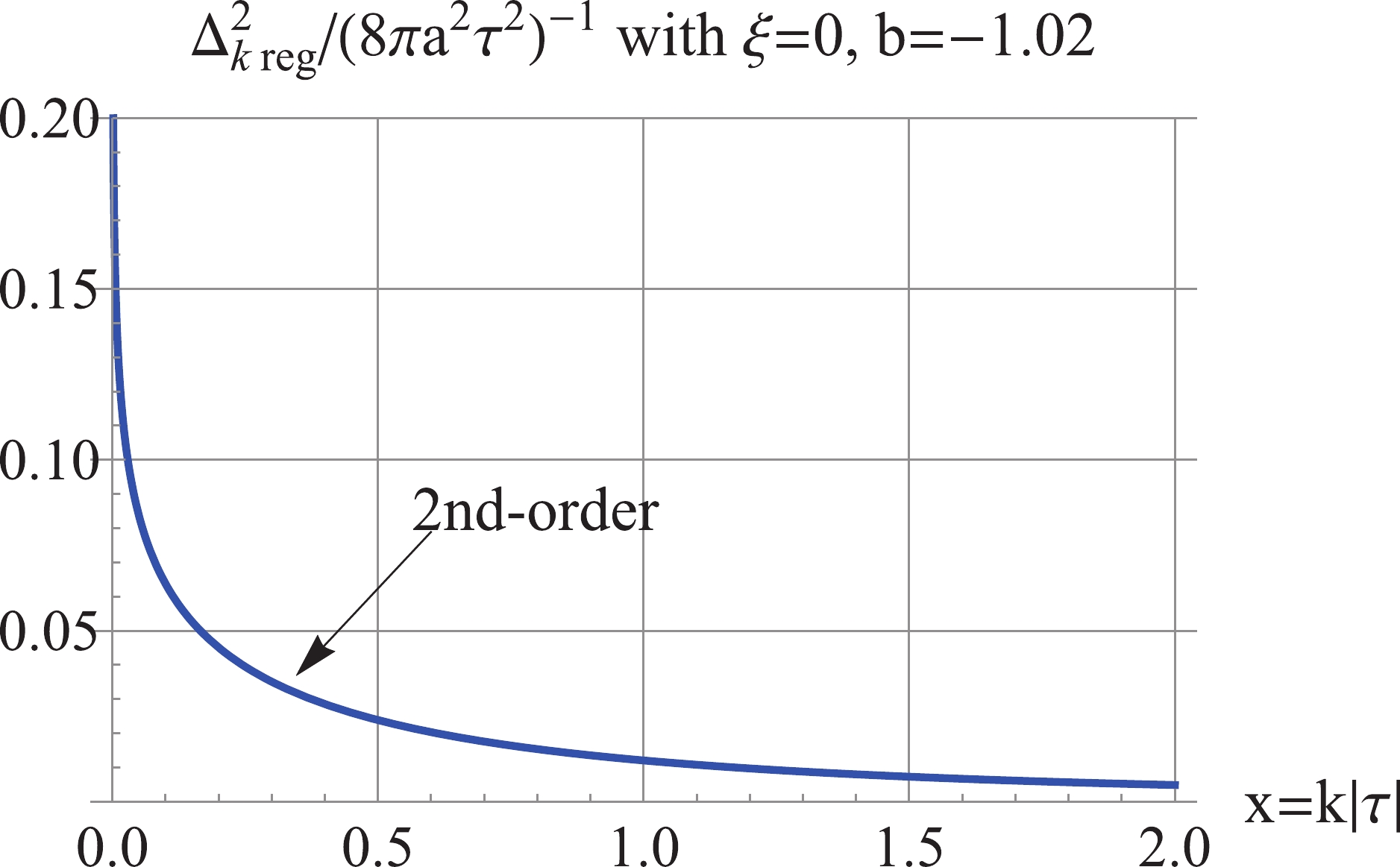
Figure 3. (color online) For
$ \xi = 0 $ ,$ b = -1.02 $ : the 2nd-order$\Delta_{k\,\rm reg}^2$ is UV convergent and IR divergent.
Figure 4. (color online) Red Dash: the 4th-order regularized
$\rho_{k\,\rm reg}$ is negative, Blue Solid: the 6th-order regularized$\rho_{k\,\rm reg}$ is positive, and$ k^{-4} $ UV convergent at high k. The model$ b = -1.02 $ and$ \xi = 0 $ .$ \frac{5 (b-2) (b-1) b^2 (b+1) (b+2)}{16 x^2} , $

(71) which is negative for
$ b = -1.02 $ . This is the phenomenon of negative spectra previously mentioned around Eqs. (33) and (34). To obtain a positive spectral energy density, we proceed to compute the 6th-order regularized$\rho_{k\,\rm reg}$ in Eq. (34), which is dominated by the fifth term of (30). As a result, the 6th-order regularized$\rho_{k\,\rm reg}$ is positive and UV-convergent, as shown in Fig. 4. As for the IR divergences in the regularized spectra, we adopt the inside-horizon scheme [32], as follows. The UV divergences come from the high k-modes; whereas, the low k-modes do not cause UV divergence. Therefore, only the short wavelength modes need to be regularized inside the horizon during the expansion ($ k \gtrsim 1/|\tau_1| $ , where$ \tau_1 $ is a fixed time during the expansion), and the long wavelength modes outside the horizon remain unchanged. Under this scheme, UV divergences are removed and IR divergences are avoided. Thus, for the case$ b = -1.02 $ under consideration, the spectral energy density is regularized by$ {\rho _k}{(\tau )_{\rm reg}} = \left\{ {\begin{array}{*{20}{c}} {{\rho _k} - {\rho _{k\; A6}},\; \; }&{{\rm{ for}}\;k \geqslant \dfrac{1}{{|{\tau _1}|}},}\\ {{\rho _k},\; \; \; \; \; }&{{\rm{ for}}\;k < \dfrac{1}{{|{\tau _1}|}}.} \end{array}} \right. $

(72) The regularization is performed instantaneously at a fixed
$ \tau_1 $ . The result is plotted in Fig. 5. Thus, IR divergence is avoided, a positive UV- and IR-convergent spectral energy density is achieved, and the regularized energy density is$\rho_{\rm reg} = \int_0^\infty \rho_{k\,\rm reg} \frac{{\rm d}k}{k} = 0.622 \frac{(b/a_0)^4}{16\pi}$ at$ |\tau| = 1 $ .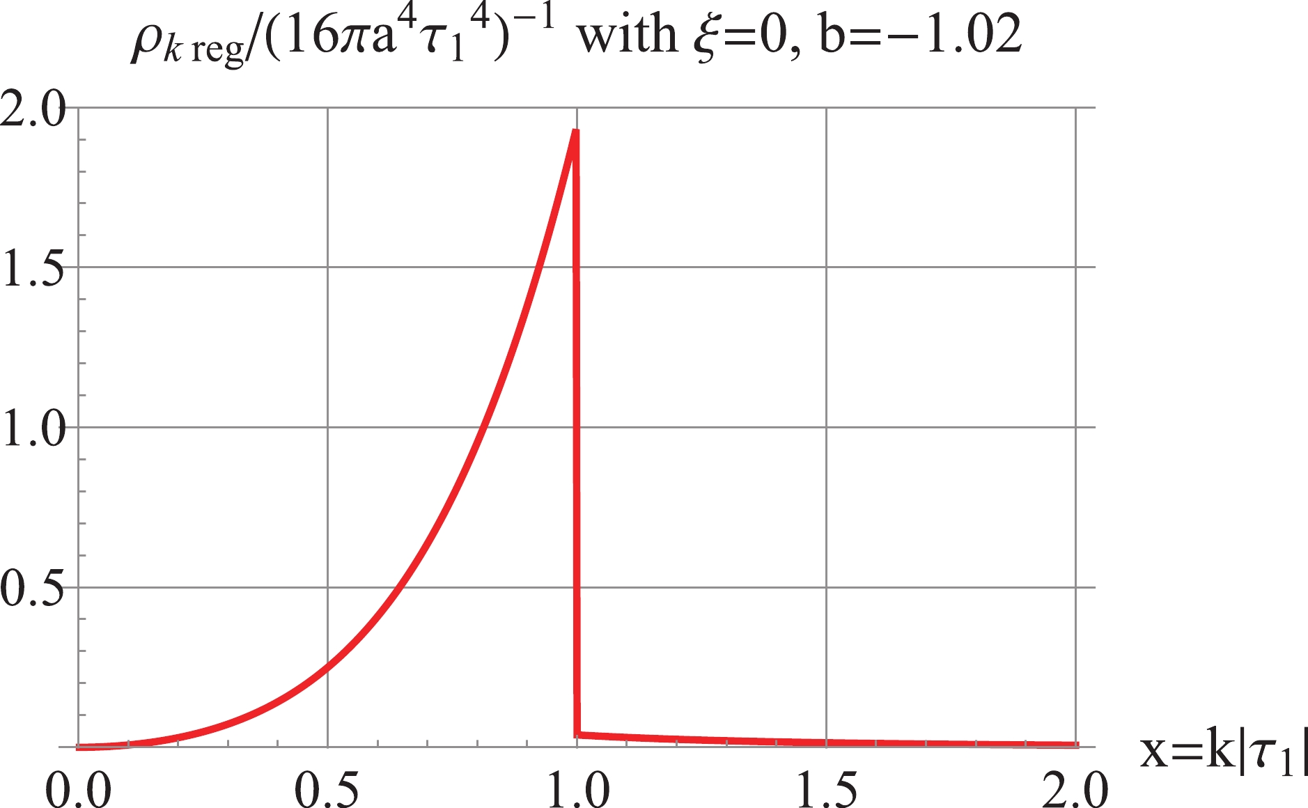
Figure 5. (color online) For
$ \xi = 0 $ ,$ b = -1.02 $ : the inside-horizon regularization for$\rho_k(\tau)_{\rm reg}$ according to Eq. (72). The plot is at a time$ |\tau_1| = 1 $ for illustration.For the model
$ b = -0.98 $ , the 2nd-order regularized power spectrum is dominated by the third term of (15) and is negative, as shown in Fig. 6. Thus, we proceed to calculate the 4th-order regularized power spectrum according to Eq. (18), which is positive, UV-convergent, and dominated by the fourth term of (15), as shown in Fig. 6. To avoid the IR divergence caused by the 4th-order regularization, we apply the inside-horizon scheme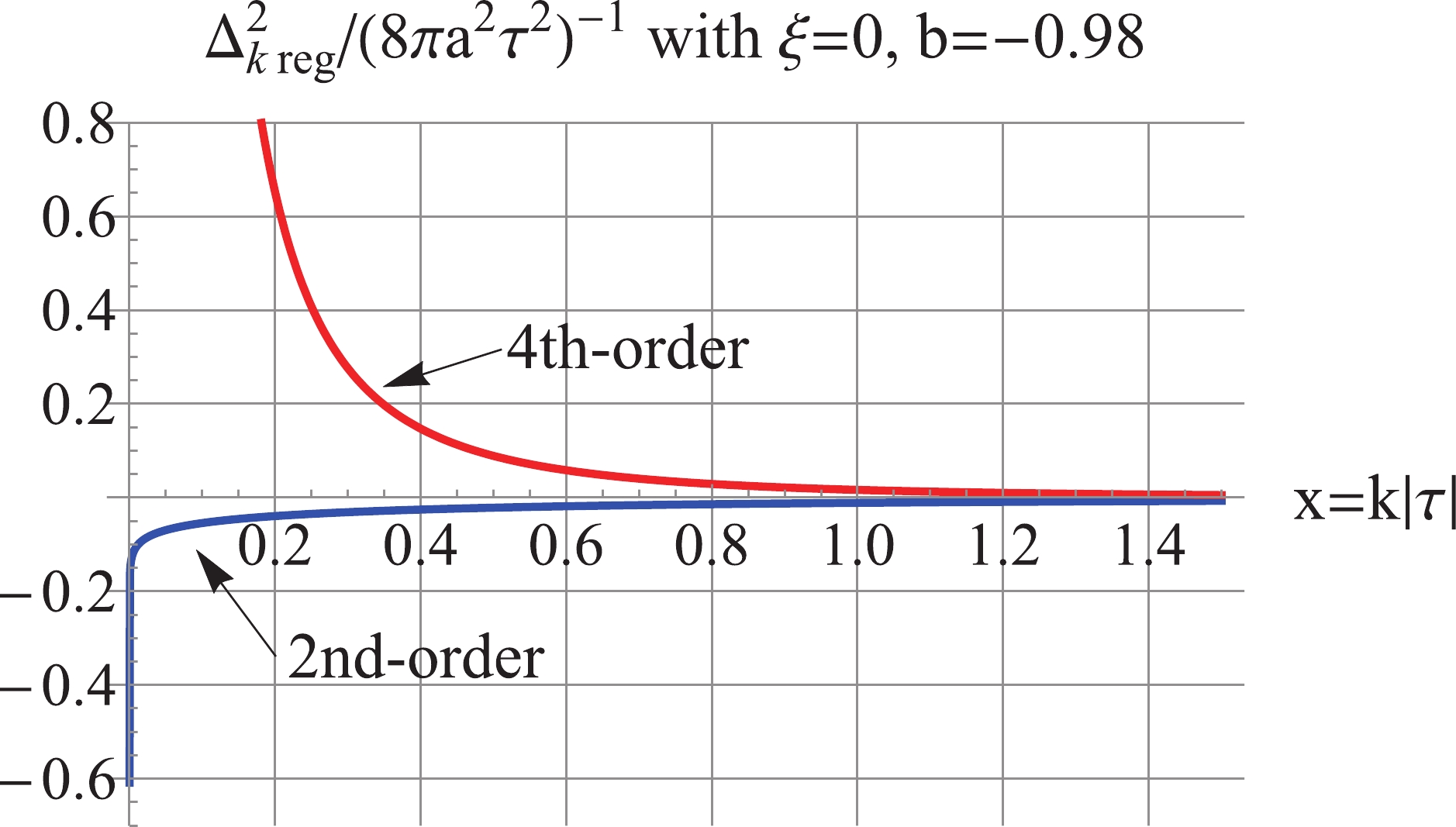
Figure 6. (color online) For
$ \xi = 0, b = -0.98 $ : the 2nd-order$\Delta_{k\,\rm reg}^2$ is negative; the 4th-order$\Delta_{k\,\rm reg}^2$ is UV convergent and IR divergent.$ \Delta _k^2{(\tau )_{\rm reg}} = \frac{{{k^3}}}{{2{\pi ^2}{a^2}}}\left\{ {\begin{array}{*{20}{c}} {(|{v_k}{|^2} - |v_k^{(4)}{|^2}),{\mkern 1mu} {\mkern 1mu} }&{{\rm{ for}}\;k \geqslant \dfrac{1}{{|{\tau _1}|}},}\\ {|{v_k}{|^2},{\mkern 1mu} {\mkern 1mu} {\mkern 1mu} {\mkern 1mu} {\mkern 1mu} }&{{\rm{ for}}\;k < \dfrac{1}{{|{\tau _1}|}}.} \end{array}} \right. $

(73) The resulting power spectrum is plotted in Fig. 7. Accordingly, the IR divergence is avoided, and a positive UV- and IR-convergent power spectrum is achieved. By the Fourier transformation of (73) according to the formula (12), we obtain the corresponding regularized Green's function
$G({{{r}}}- {{{r}}}')_{\rm reg}$ , which is UV-finite and IR-convergent, as shown in Fig. 8. The 4th-order regularized spectral energy density is positive and UV-convergent, as plotted in Fig. 9, and the regularized energy density is$\rho_{\rm reg} = \int_0^\infty \rho_{k\,\rm reg} \frac{{\rm d}k}{k} = 0.228\frac{(b/a_0)^4}{16\pi}$ at$ |\tau| = 1 $ . The above two examples show that the inside-horizon scheme is effective in avoiding IR divergences.
Figure 7. (color online) For
$ \xi = 0 $ ,$ b = -0.98 $ : the inside-horizon regularization for$\Delta^2_{k\,\rm reg}$ according to Eq. (73).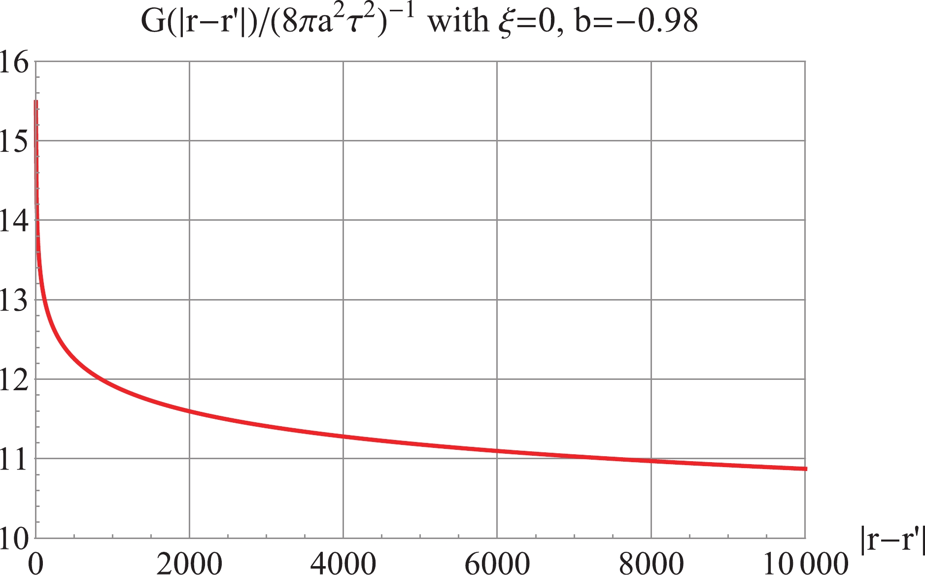
Figure 8. (color online) For
$ \xi = 0 $ ,$ b = -0.98 $ : the regularized Green's function$G(|{{{r}}}- {{{r}}}'|)_{\rm reg}$ , is Fourier transform of the regularized power spectrum in Fig. 7.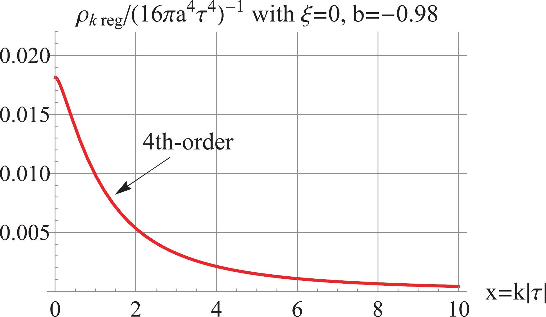
Figure 9. (color online) For
$ \xi = 0, b = -0.98 $ : the 4th-order$\rho_{k\,\rm reg}$ is positive, UV convergent and IR log divergent. -
Now, we explore adiabatic regularization for a general coupling
$ \xi $ , and search for proper regularization schemes that would yield the nonnegative UV- and IR-convergent spectra$ \Delta^2_{k } $ and$ \rho_k $ . We shall consider several values of b in various interesting cosmological models. By the minimal subtraction rule, the 2nd-order regularization for$ \Delta^2_{k } $ and the 4th-order regularization for$ \rho_k $ are default, and we shall attempt higher-order regularization when a negative spectrum appears.First, we consider
$ b = 1 $ for the RD stage with a general$ \xi $ . The analysis between (52)-(58) is also valid for a general$ \xi $ , and the results are$\Delta^2_{k\,\rm reg } = \rho_{k\,\rm reg } = p_{k\,\rm reg} = 0$ .Next, we consider
$ b = 2 $ for the MD stage with a general$ \xi $ . For illustration,$ \xi = \frac{1}{8} $ is used in the following, other values of$ \xi $ can be analyzed in the same fashion. As shown in Fig. 10, the 2nd-order regularized$\Delta_{k\,\rm reg}^2$ is negative, dominated by the third term of Eq. (15), and the 4th-order regularized$\Delta_{k\,\rm reg}^2$ is positive and UV-convergent, but IR-divergent. As shown in Fig. 11, the 4th-order regularized$\rho_{k\,\rm reg}$ is negative, dominated by the fourth term in Eq. (30), while the 6th-order regularized$\rho_{k\,\rm reg}$ is positive, dominated by the fifth term of (30).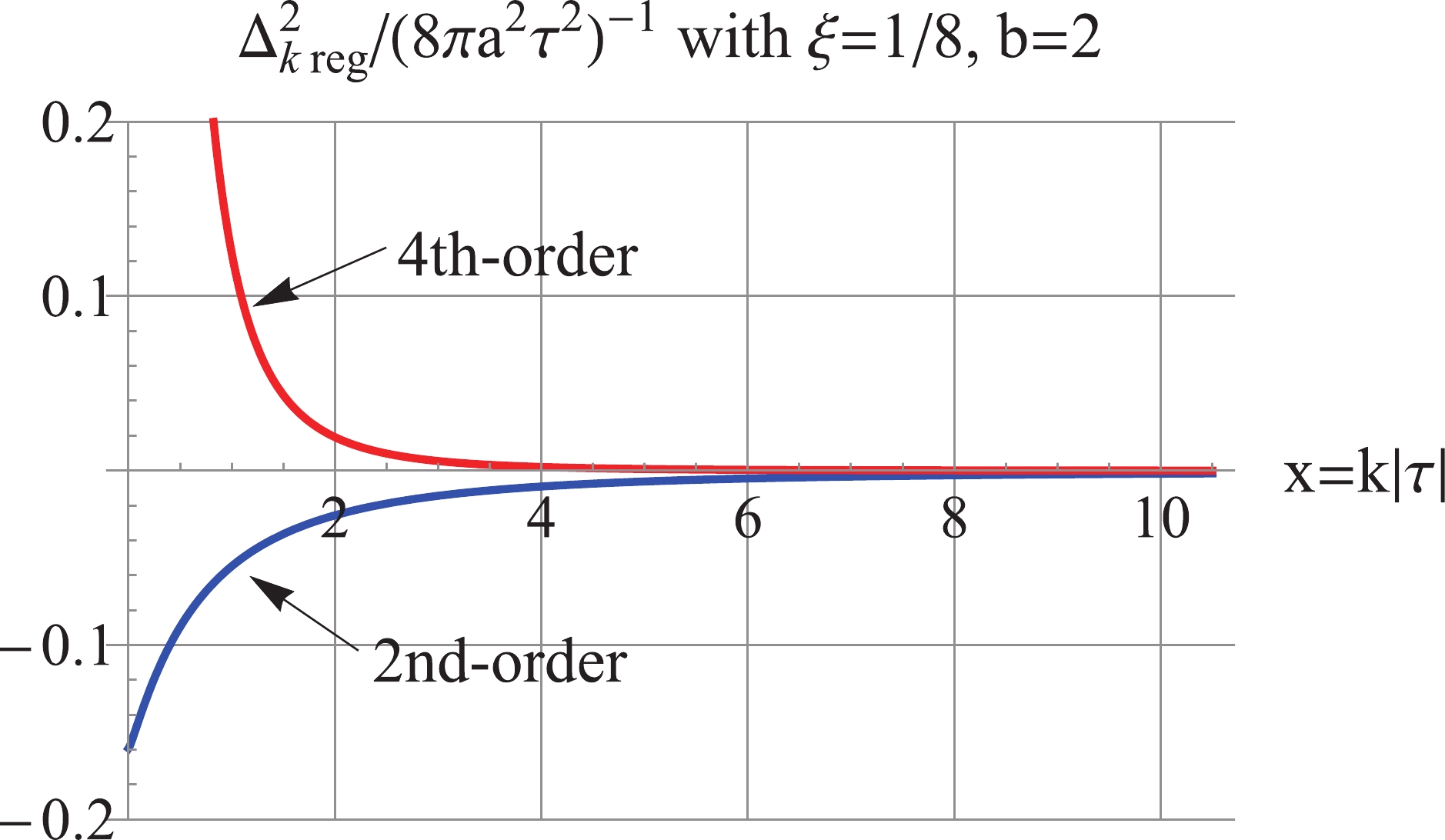
Figure 10. (color online) For
$ b = 2 $ and$ \xi = 1/8 $ , the 2nd-order regularized$ \Delta_k^2 $ is negative, and the 4th-order regularized$ \Delta_k^2 $ is positive, and UV convergent.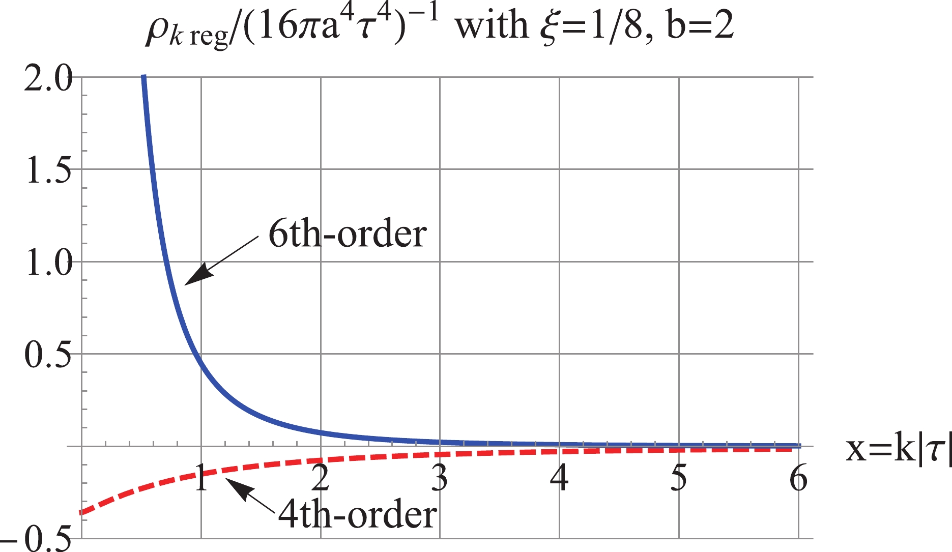
Figure 11. (color online) For
$ b = 2 $ and$ \xi = \frac18 $ , Red Dashed: the 4th-order regularized$\rho_{k\,\rm reg}$ is negative; Blue Solid: the 6th-order regularized$\rho_{k\,\rm reg}$ is positive, and$ k^{-4} $ UV convergent at high k.Then, we consider
$ b = -1 $ in de Sitter space. We plot the regularized power spectra for$ \xi = \frac{1}{8} $ in Fig. 12, the 2nd-order regularized$\Delta_{k\,\rm reg}^2$ is negative, while the 4th-order regularized$\Delta_{k\,\rm reg}^2$ is positive and UV-convergent, but IR-divergent. As shown in Fig. 13, the 4th-order regularized$ \rho_k $ is positive and UV- and IR-convergent. (Here$ \frac{2a''' a'}{a^2} -\frac{a''\, ^2}{a^2}-\frac{4a'' a'\,^2}{a^3} = 0 $ for de Sitter space, so that the 2nd-order subtraction term (B35) is equal to the 4th-order (B37), and the 2nd-order regularized$ \rho_k $ is equal to that of the 4th-order.)
Figure 12. (color online) For
$ b = -1 $ and$ \xi = \frac18 $ , the 2nd-order regularized$ \Delta_k^2 $ is negative, the 4th-order regularized$ \Delta_k^2 $ is positive and UV convergent.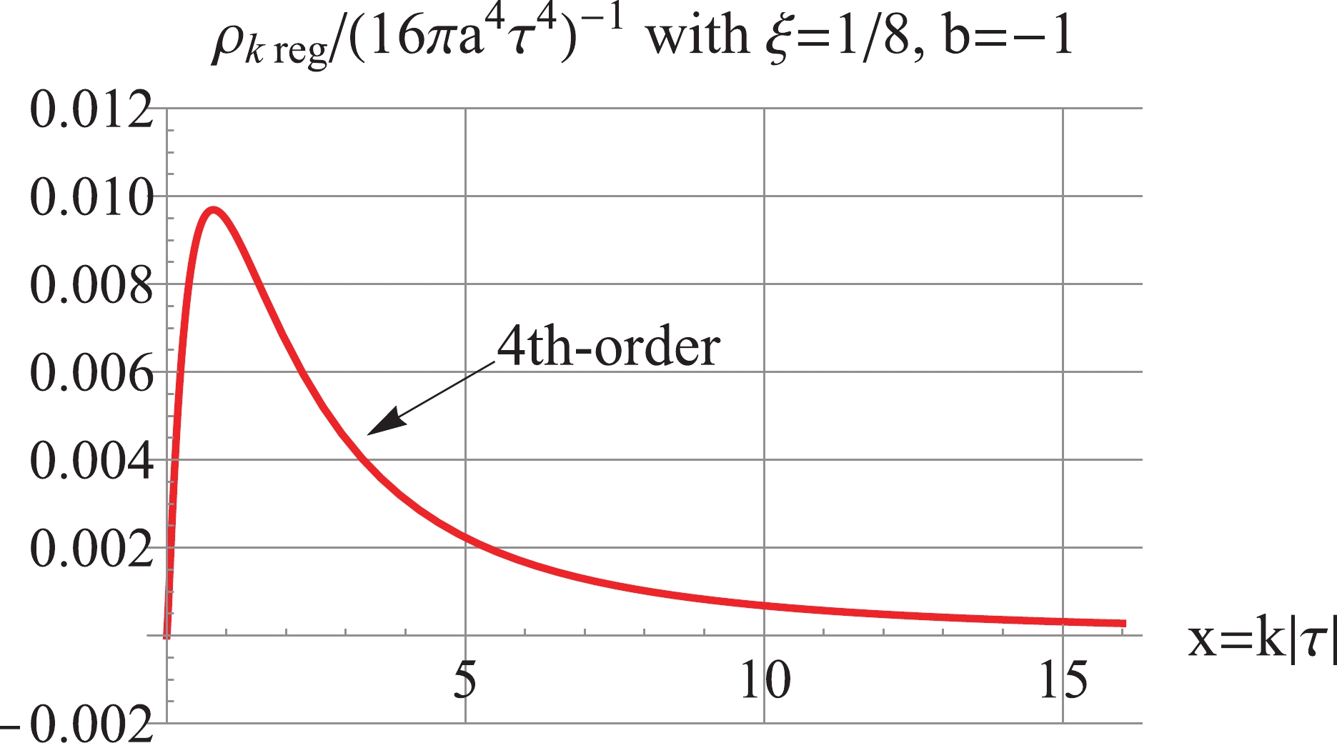
Figure 13. (color online) For
$ b = -1 $ and$ \xi = \frac18 $ , the 4th-order regularized$ \rho_k $ is positive and UV convergent.Finally, we consider the quasi de Sitter inflation model with
$ b = -0.98 $ and$ \xi = \frac{1}{8} $ . As shown in Fig. 14, the 2nd-order regularized$ \Delta_k^2 $ is negative, and the 4th-order regularized$ \Delta_k^2 $ is positive and UV-convergent but IR-divergent. Furthermore, Fig. 15 shows that the 4th-order regularized$ \rho_k $ is positive, IR-finite, and UV-convergent. For the model with$ b = -1.02 $ and$ \xi = \frac{1}{8} $ , as shown in Fig. 16, the 2nd-order regularized$ \Delta_k^2 $ is negative; the 4th-order regularized$ \Delta_k^2 $ is positive and UV-convergent, but IR-divergent. Fig. 17 shows that the 4th-order regularized$ \rho_k $ is positive and UV-convergent, but IR-log-divergent.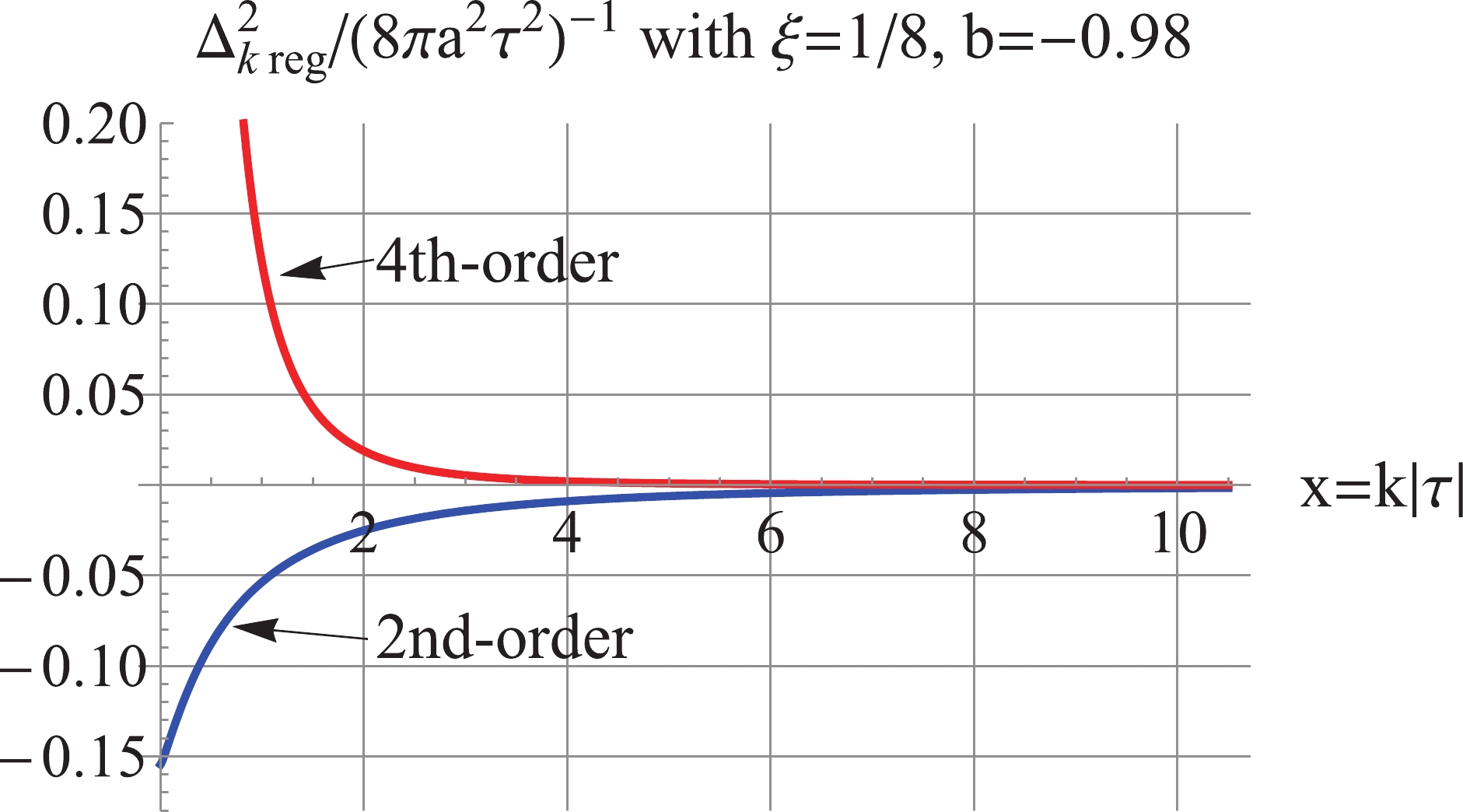
Figure 14. (color online) For
$ b = -0.98 $ and$ \xi = 1/8 $ , the 2nd-order regularized$ \Delta_k^2 $ is negative, the 4th-order regularized$ \Delta_k^2 $ is positive and UV convergent.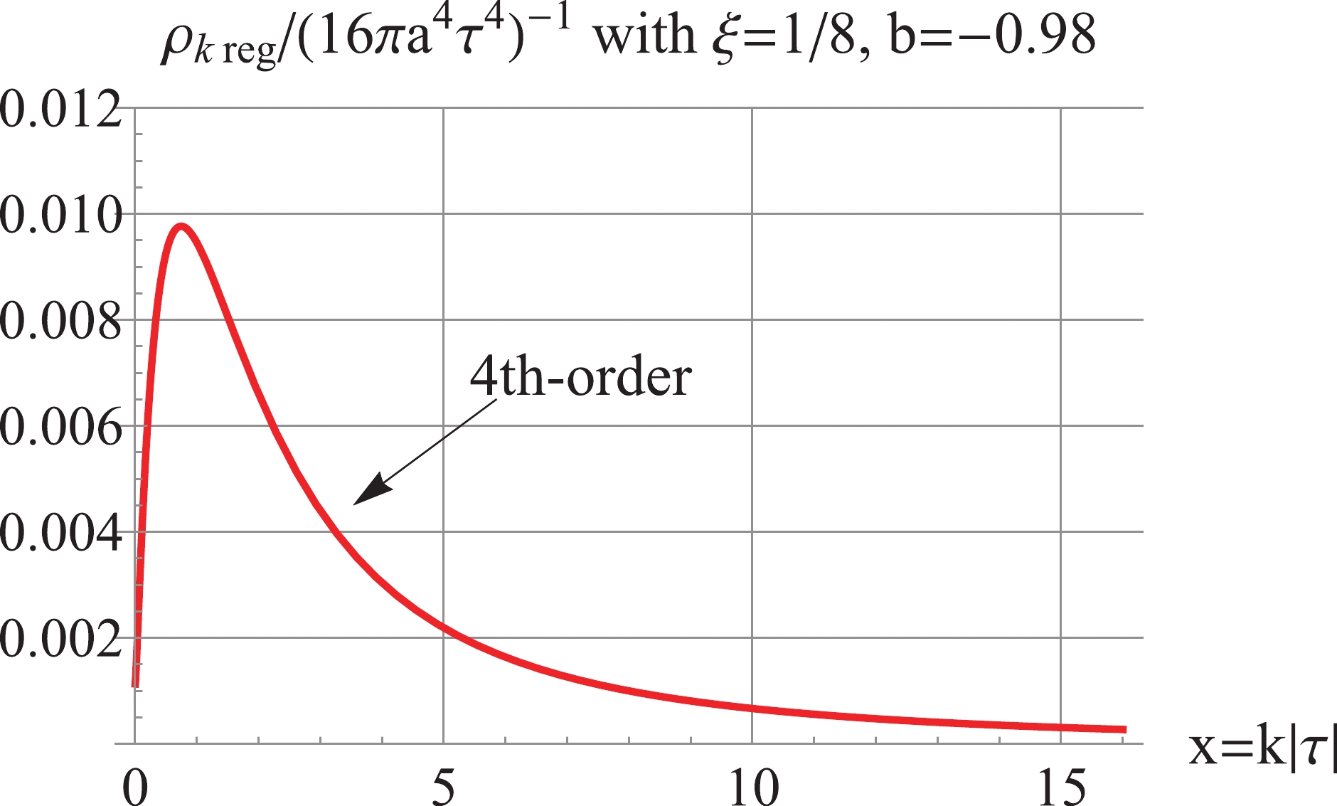
Figure 15. (color online) For
$ b = -0.98 $ and$ \xi = 1/8 $ , the 4th-order regularized$ \rho_k $ is positive and UV convergent.
Figure 16. (color online) For
$ b = -1.02 $ and$ \xi = 1/8 $ , The 2nd-order regularized$ \Delta_k^2 $ is negative, and the 4th-order regularized$ \Delta_k^2 $ is positive and UV convergent.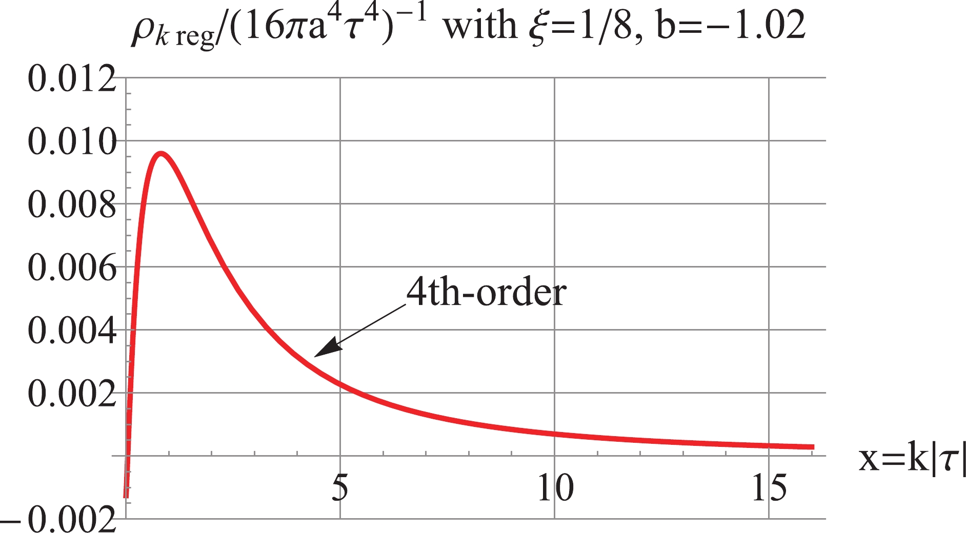
Figure 17. (color online) For
$ b = -1.02 $ and$ \xi = \frac{1}{8} $ , the 4th-order regularized$\rho_{k\,\rm reg}$ is positive at high k.In the above, when IR divergence appears, the inside-horizon scheme can be applied, as in Sec. 4, the details of which are not discussed to save room. Hence, for general
$ \xi $ and b, positive UV- and IR-convergent power spectrum and spectral energy density can be achieved. -
We have studied adiabatic regularization of a massless scalar field in general RW spacetimes with a coupling
$ \xi $ (in the specific range$ 0 \leq \xi \leq \frac{1}{6} $ for this paper), and this extends our previous study in de Sitter space [17]. The analytical expressions of the power spectrum, the corresponding Green's function, and the spectral stress tensor were presented, all of which contain UV divergences. Our goal is to find the appropriate schemes of regularization that will achieve nonnegative UV- and IR-convergent power spectrum and spectral energy density. Adiabatic regularization respects the covariant conservation of the stress tensor to each order. For the massless field, the UV divergences are generally removed when the power spectrum is regularized to the 2nd-order, and the stress tensor to the 4th order. The nonnegativeness, however, is not always ensured by the conventional prescription, and this is our main concern in this paper. Through several examples, we have found that there is no regularization scheme of fixed-order that would work for all couplings and all RW spacetimes. An adequate scheme depends upon the coupling$ \xi $ and the expansion index b.Several interesting cases are very simple. For the conformally coupled massless scalar field in Sec. 3, we found that the regularized power spectrum and stress tensor are zero, and no trace anomaly exists in general RW spacetimes. The regularization of the field with conformal symmetry effectively amounts to the normal ordering in the Minkowski spacetime. This result is a generalization of our previous work on de Sitter space [17]. We have also explicitly identified the mistakes of Refs. [11, 14] on a massless field. Most literature on the trace anomaly started with a massive field, adopted the 4th-order regularization on the stress tensor, and then took the massless limit. As we showed in detail in Ref. [17], for a massive scalar field, 4th-order regularization is not appropriate, because it will lead to an unphysical, negative spectral energy density, which is a vital shortcoming unnoticed in the previous literature. In fact, for a conformally coupled massive scalar field, 0th-order regularization [17] is the correct scheme, as it not only removes all the UV divergences, but also gives a positive spectral energy density, and the resulting stress tensor is zero in the massless limit, agreeing with the present paper. Therefore, the trace anomaly claimed in literature is an artifact caused by the inadequate 4th-order regularization.
Another simple case is minimal coupling where
$ \xi = 0 $ , as in Sec. 4, the regularized spectra are zero for$ b = 0, \pm 1, 2 $ , corresponding to the Minkowski spacetime, the de Sitter space, the RD stage, and the matter-dominated stage. In the above simple cases, we also conducted direct regularization of the Green's functions in position space, and found that the regularized Green's functions are zero as well, confirming the zero spectra by adiabatic regularization. In particular, for the RD stage, the regularized spectra are also zero for any coupling$ \xi $ . This is because during the RD stage, the scalar curvature$ R = 0 $ so that the wave equation (3) with arbitrary$ \xi $ is also conformal to those in the Minkowski spacetime.For the cases of general
$ \xi $ and b in Sec. 5, we found that the regularized spectra of the massless scalar field can be negative under the conventional regularization. To avoid the negative spectra, we performed higher-order regularization to the pertinent spectrum. Specifically, if the power spectrum is negative under the 2nd-order regularization, we calculate its 4th-order regularization, and similarly if the spectral energy density is negative under the 4th-order regularization, we calculate its 6th-order regularization. In fact, the resulting higher-order regularization spectrum will usually become positive for the RW spacetimes commonly used in cosmology. In some rarely used RW spacetimes, the 6th-order regularized spectral energy density may still be negative, then we go to the 8th-order, which will eventually yield a positive spectral energy density.A massless field may carry IR divergence in the unregularized spectra, as summarized in (21), (41), and (42). Refs. [34, 35] present studies regarding avoiding the IR divergence in the unregularized spectra. In this paper, we have analyzed the IR divergences caused by regularization. In particular, IR divergence occurs when going to higher-order regularization for general
$ \xi $ and b. These new IR divergences can be avoided by the inside-horizon scheme of regularization, as demonstrated by the examples in Fig. 5 and Fig. 7. The details of the inside-horizon scheme were discussed in Ref. [32], and we only mention the following two related points. First, the scalar field considered in this paper is linear, and its k-modes are independent of each other, unlike the nonlinear fields [36]. Under the inside-horizon scheme, each regularized short wavelength mode respects the covariant conservation to pertinent order, the unregularized long wavelength modes also respect the covariant conservation. Thus, the total stress tensor respects the covariant conservation by the inside-horizon scheme. Second, the long wavelength modes outside the horizon correspond to the waveband of the observed CMB temperature anisotropies and polarization [31, 32]. When the scalar field is used to model the cosmological perturbations, the inside-horizon scheme reserves the spectra perturbations of the long wavelength band, so that the observed primordial spectrum will not be affected by any scheme of regularization.Through these detailed investigations, we conclude that for a coupled massless scalar field in general RW spacetimes, the nonnegative UV- and IR-convergent power spectrum and spectral energy density can be achieved by adiabatic regularization, with the help of a higher-order scheme and the inside-horizon scheme when necessary.
The authors thank A. Marciano for valuable discussions.
-
We list some asymptotic expressions following the analytical solution for a general RW spacetime, which are used in the context.
At high
$ k $ , the mode$ v_k $ of (6) approaches to$ \begin{split} v_{k } \simeq & \frac{1}{\sqrt{2k}}{\rm e}^{{\rm i}x } \Big(1 + i\frac{(4\nu^2-1)}{8x} -\frac{(16\nu^4 -40\nu^2 +9)}{128 x^2} -i\frac{(64\nu^6 -560\nu^4 +1036\nu^2 -225)}{3072 x^3} + \frac{(256\nu^8-5376\nu^6+31584 \nu^4 -51664 \nu^2 +11025 )}{98304 x^4} \\ & + i \frac{ \left(-1024 \nu ^{10}+42240 \nu ^8-561792 \nu ^6 +2764960 \nu ^4-4228884 \nu ^2+893025\right)}{3932160 x^5} + ... \Big) , \end{split}\tag{A1} $

(A1) where the first term corresponds to the positive-frequency mode in Minkowski spacetime, and other terms are due to expansion effects. The squared mode at high k is
$ \begin{split} |v_k|^2 =& \frac{\pi x}{4k} \big| H^{(2)}_{\nu} ( x) \big|^2 = \frac{1}{2k} \Big( 1+ \frac{4\nu^2 -1}{8 x^2} +\frac{3(16\nu^4 -40\nu^2 +9)}{128 x^4} \\ & +\frac{5(2\nu-5)(2\nu-3)(2\nu-1)(2\nu+1)(2\nu+3)(2\nu+5)}{1024 x^6} + ... \Big). \end{split}\tag{A2} $

(A2) The time derivatives to the 4th adiabatic order are given by
$ \tag{{\text{A3}}} |v_k'|^2 = k \left(\frac{1}{2} - \frac{ ( 4 \nu^2 -1)}{16 x^2} - \frac{ (16\nu^4 - 104\nu^2 +25)}{256 x^4} -\frac{ (64\nu^6 -2096 \nu^4 +4876\nu^2 -1089)}{2048 x^6} + ... \right), \quad\quad\quad\quad\quad\quad\quad\quad\quad\quad\quad\quad\quad\quad\quad\quad\quad\quad\quad\quad\quad\quad $

$ \tag{{A4}} \begin{aligned}[b] |\Big(\frac{v_k}{a}\Big)'|^2 =& b^{-2}H^2\Big( \frac{x^2}{2 k} +\frac{8 b^2+1-4 \nu ^2}{16 k} -\frac{16 \nu ^4 -\left(64 b^2+128 b+104\right) \nu ^2 +(16 b^2+32 b+25)}{256 k x^2} \\ &+\frac{(216 b^2+864 b+1089) -\left(960 b^2+3840 b+4876\right) \nu ^2 +\left(384 b^2+1536 b+2096\right) \nu ^4 -64 \nu ^6}{2048 k x^4} +...\Big) . \end{aligned} $

From these, the high-k expansions of
$ \rho_k $ and$ p_k $ can be obtained, as in Eqs. (30) and (31) in the context.At low k, the mode
$ v_k $ of (6) and the related squared modes are given by$\tag{A5} v_{k } \simeq \Big(\frac{x}{2}\Big)^{-\nu + \frac12} \frac{ \Gamma(\nu)}{\sqrt{2 \pi k}} {\rm e}^{{\rm i} \frac{\pi}{2}(\nu - \frac12) } , $

(A5) $\tag{A6} |v_k|^2 \simeq x^{-2\nu } |\tau| \frac{ 2^{2\nu-2} \Gamma(\nu)^2 }{ \pi }, $

(A6) $\tag{A7} | \frac{v_k}{a}|^2 \simeq a_0^{-2}x^{-2\nu } |\tau|^{1-2b} \frac{ 2^{2\nu-2} \Gamma(\nu)^2 }{ \pi }, $

(A.7) and the time derivatives are
$\tag{A8} v_k' \simeq \frac{|\tau|}{\tau} \Big(\frac{x}{2}\Big)^{-\nu - \frac12} k^{1/2} \frac{ \Gamma(\nu)-2\Gamma(\nu +1)}{4 \sqrt{2 \pi }} {\rm e}^{{\rm i} \frac{\pi}{2}(\nu - \frac12) } , $

(A.8) $\tag{A9} |v_k'|^2 \simeq \Big(\frac{x}{2}\Big)^{-2\nu - 1} k \frac{ (\Gamma(\nu)-2\Gamma(\nu +1))^2 }{32 \pi}, $

(A.9) $\tag{A10} \Big(\frac{v_k}{a}\Big)' = \frac{|\tau|}{\tau} a_0^{-1} \left(\frac{x}{2}\right)^{-\frac{1}{2}-b-\nu} k^{\frac{1}{2}+b} \frac{(1-2 b) \Gamma (\nu )-2 \Gamma (\nu +1) }{ 2^{2+b} \sqrt{2 \pi }} {\rm e}^{{\rm i} \frac{\pi}{2} (\nu -\frac{1}{2})} , $

(A.10) $\tag{A11} \Big|\Big(\frac{v_k}{a}\Big)'\Big|^2 = a_0^{-2} x^{-2 \nu }|\tau|^{-1-2 b} \frac{ 2^{2 \nu } \Big[(1-2 b) \Gamma (\nu )-2 \Gamma (\nu +1)\Big]^2}{16 \pi }. $

(A11) From these follow the low-k expansions of
$ \rho_k $ and$ p_k $ in Eqs. (41) and (42). -
The WKB approximate solution [18, 19, 25-27, 37] of the massless scalar field equation (4) is written as the following
$\tag{B1} v_k^{(n)}(\tau) = (2W_k(\tau))^{-1/2} \exp \bigg[ -{\rm i} \int^{\tau} W_k(\tau'){\rm d}\tau' \bigg], $

(B1) where the effective frequency is
$\tag{B2} W_k(\tau) = \bigg[ k^2 + \bigg(\xi -\frac16\bigg)a^2R -\frac12 \left( \frac{ W_k '' }{ W_k} - \frac32 \bigg( \frac{W_k '}{W_k} \bigg)^2 \right) \bigg]^{1/2}. $

(B2) The WKB solution of
$ W_k $ is obtained by iteratively solving (B2) to a desired adiabatic order. Take the 0th-order [25],$\tag{B3} W_k^{(0)} = k , $

(B3) and the 0th-order adiabatic mode
$\tag{B4} v_k^{(0)}(\tau) = (2 k)^{-1/2} {\rm e}^{-{\rm i} \int^{\tau}k {\rm d}\tau'} . $

(B4) The 0th-order quantities that appear in the 0th-order subtraction terms are
$\tag{B5} |v_k^{(0)}|^2 = \frac{1}{2W_k^{(0)}} = \frac{1}{2k}, $

(B5) $\tag{B6} |v_k^{(0)\prime}|^2 = \frac{1}{2}\left( \frac{(W_k^{(0)\prime})^2}{4(W_k^{(0)})^{3}}+W_k^{(0)} \right) = \frac{k}{2} , $

(B6) $\tag{B7} v_k^{(0)\prime}v_k^{(0)*}+v_k^{(0)}v_k^{(0)*\,\prime} = 0 , $

(B7) $\quad\quad\;\quad\;\quad\tag{B8} \begin{split} \Big|\Big(\frac{v^{(0)}_k}{a}\Big)' \Big|^2 =& \frac{1}{a^2} \Big( |v^{(0)}_k \, ' |^2 - \frac{a'}{a} (v_k ^{(0)}\, ' v_k^{(2)}\, ^* + v_k^{(0)} v_k^{(2)}\, ^*\, ') \\&+\Big(\frac{a'}{a}\Big)^2 |v^{(0)}_k|^2 \Big) = \frac{1}{a^2} \Big( \frac{k}{2} +\Big(\frac{a'}{a}\Big)^2 \frac{1}{2k} \Big) . \end{split}\tag{B8} $

(B8) These 0th-order subtraction terms are independent of
$ \xi $ . The 2nd-order adiabatic mode is$ \tag{B9}v_k^{(2)}(\tau) = (2W_k^{(2)}(\tau))^{-1/2} {\rm e}^{ -{\rm i} \int^{\tau} W_k^{(2)}(\tau'){\rm d}\tau'} , $

(B9) The 2nd-order effective frequency is given by the first iteration of (B2)
$\tag{B10} W_k^{(2)} = \left[ k^2 + \Big(\xi -\frac16\Big)a^2R -\frac12 \left( \frac{ W^{(0)}_k\, '' }{ W^{(0)} _k } - \frac32 \Big( \frac{W^{(0)}_k\, '}{W^{(0)}_k} \Big)^2 \right) \right]^{\frac12} \, . $

(B10) Keeping only two time derivatives of
$ a(\tau) $ gives$\tag{B11} W_k^{(2)} = \sqrt{k^2+6 \Big(\xi -\frac16\Big) \frac{a''}{a}} \simeq k + 3 \Big(\xi-\frac16\Big)\frac{1}{k } \frac{a''}{a}, $

(B.11) $\tag{B12} (W_k^{(2)})^{-1} \simeq \frac{1}{k} - 3 \Big(\xi-\frac16\Big) \frac{a''/a}{k^{3}} . $

(B.12) The 2nd-order subtraction term for the power spectrum is
$\tag{B13} |v^{(2)}_k|^2 = \frac{1}{2 W_k^{(2)}} = \frac{1}{2k} - \frac{3}{2} \Big(\xi-\frac16\Big) \frac{a''/a}{k^{3}}. $

(B13) The 2nd-order subtraction term for
$ \rho_k $ and$ p_k $ also involves the following terms$\tag{B14} |v^{(2)}_k \, ' |^2 = \frac12 \Bigg( \frac{ (W_k^{(2)\, '})^2 }{4 (W_k^{(2)})^{3} } + W_k^{(2)} \Bigg) = \frac{k}{2} +\Big(\xi-\frac16\Big)\frac{3 a''}{2 k a } , $

(B14) $\tag{B15} v_k ^{(2)}\, ' v_k^{(2)}\, ^* + v_k^{(2)} v_k^{(2)}\, ^*\, ' = - \frac{ W_k^{(2)\, '} }{2 ( W_k^{(2)})^2 } \simeq 0 , $

(B15) $\tag{B16} \begin{aligned}[b] \Big|\Big(\frac{v^{(2)}_k}{a}\Big)' \Big|^2 =&\frac{1}{a^2} \Big( |v^{(2)}_k \, ' |^2 - \frac{a'}{a} (v_k ^{(2)}\, ' v_k^{(2)}\, ^* + v_k^{(2)} v_k^{(2)}\, ^*\, ') +\Big(\frac{a'}{a}\Big)^2 |v^{(2)}_k|^2 \Big) \\ =& \frac{k}{2a^2}+\frac{1}{2k a^2}\Big(\frac{a'}{a}\Big)^2 +\Big(\xi-\frac16\Big)\frac{3}{2k } \frac{a''}{a^3} . \end{aligned} $

(B16) These 2nd-order subtraction terms are dependent on
$ \xi $ . A very important property of a massless scalar field is that$ W_k^{(2)} = W_k^{(0)} = k $ for the conformal coupling$ \xi = \frac16 $ . Actually,$ W_k^{(n)} = W_k^{(0)} = k $ holds for an arbitrary nth-order, as is implied by the iteration formula (B2).The 4th-order adiabatic mode is defined by
$\tag{B17} v_k^{(4)}(\tau) = (2W_k^{(4)}(\tau))^{-1/2} {\rm e}^{-{\rm i} \int^{\tau} W_k^{(4)}(\tau'){\rm d}\tau'} , $

(B17) the 4th-order effective frequency is given by the iteration
$\tag{B18} W_k^{(4)} = \left[ k^2 + \Big(\xi -\frac16\Big)a^2R -\frac12 \left( \frac{ W^{(2)}_k\, '' }{ W^{(2)} _k } - \frac32 \Big( \frac{W^{(2)}_k\, '}{W^{(2)}_k} \Big)^2 \right) \right]^{\frac12} . $

(B18) Keeping up to four time derivatives, the following are obtained
$\tag{B19} \begin{aligned}[b] W_k^{(4)} =& k + \frac{3(\xi-\frac16) }{k } \frac{a''}{a} -\frac92 \Big(\xi-\frac16 \Big)^2 \frac{a''\, ^2}{a^2 k^3} \\ & - \Big(\xi -\frac{1}{6}\Big) \frac{3}{4 k^3} \Big( \frac{ a''''}{a}-\frac{ a''\, ^2}{a ^2} -\frac{2 a''' a' }{a ^2}+\frac{2 a'\, ^2 a''}{ a^3} \Big) , \end{aligned} $

(B19) and
$\tag{B20} \begin{aligned}[b] (W_k^{(4)})^{-1} =& \frac{1}{k } -3 \Big(\xi -\frac{1}{6} \Big) \frac{1}{k ^3} \frac{a''}{a} + \Big(\xi -\frac{1}{6}\Big) \frac{3}{4 k^5} \Big(\frac{a'''' }{a} -\frac{a''\, ^2}{a^2}\\& + 2 \frac{a'\, ^2 a''}{a^3} -2 \frac{a''' a'}{a^2}\Big) + \Big(\xi -\frac{1}{6}\Big)^2 \, \frac{27}{2 k^5} \frac{a''\,^2}{a^2} . \end{aligned} $

(B20) Then,
$\tag{B21} |v^{(4)}_k|^2 = (2 W_k^{(4)})^{-1} , $

(B21) $\tag{B22} \begin{aligned}[b]|v^{(4)}_k \, ' |^2 =& \frac{k}{2} +(\xi-\frac16)\frac{3 a''}{2 k a} - (\xi -\frac{1}{6} )^2\frac{9}{4 k^3} \frac{a''^2}{a^2} \\&- (\xi -\frac{1}{6} ) \frac{3}{8 k ^3} (\frac{ a''''}{a} -\frac{a''^2}{a^2} -\frac{2 a''' a'}{a^2} +\frac{2 a'^2 a''}{a^3} ) , \end{aligned}$

(B22) $\tag{B23} (v_k ^{(4)}\, ' v_k^{(4)}\, ^* + v_k^{(4)} v_k^{(4)}\, ^*\, ') = - \frac{ W_k^{(4)\, '} }{2 ( W_k^{(4)})^2 } = -\frac{3}{2} (\xi -\frac{1}{6}) ( \frac{ a'''}{ k^3 a}-\frac{a'a''}{ k^3 a^2 }), $

(B23) put together yields
$ \tag{B24} \begin{aligned}[b] |(\frac{v^{(4)}_k}{a})' |^2 =& \frac{1}{a^2} \Bigg[|v_k^{(4)'}|^2 -\frac{a'}{a}(v_k^{(4)'}v_k^{(4)*}+v_k^{(4)}v_k^{(4)*'}) +(\frac{a'}{a})^2|v_k^{(4)}|^2 \Bigg] \\ =& \frac{1}{a^2} \Bigg[\frac{k }{2} +\frac{1}{2 k } \frac{a'^2}{ a^2} +(\xi-\frac16)\frac{3 a''}{2 k a } -(\xi-\frac16)^2 \frac{9}{4 k^3} \frac{a''^2}{a^2} \\ &-(\xi-\frac16) \frac{3}{8 k^3}(\frac{ a''''}{a} -\frac{a''^2}{a^2} -\frac{6 a' a'''}{ a^2} +\frac{10 a'^2 a''}{ a^3}) \Bigg]. \end{aligned} $

(B24) These 4th-order subtraction terms are also dependent on
$ \xi $ . The portions up to the two time derivatives of the above reduce to the 2nd-order results.Similarly, the 6th-order adiabatic mode
$\tag{B25} v_k^{(6)}(\tau) = (2W_k^{(4)}(\tau))^{-1/2} {\rm e}^{-{\rm i} \int^{\tau} W_k^{(4)}(\tau'){\rm d}\tau'} . $

(B.25) The 6th-order effective frequency is derived by iteration
$\tag{B26} W_k^{(6)} = \left[ k^2 + (\xi -\frac16)a^2R -\frac12 \left( \frac{ W^{(4)}_k\, '' }{ W^{(4)} _k } - \frac32 \big( \frac{W^{(4)}_k\, '}{W^{(4)}_k} \big)^2 \right) \right]^{\frac12} . $

(B26) Keeping up to six time derivatives, one obtains
$\tag{B27} \begin{aligned}[b] W_k^{(6)} =& k +\frac{3 (\xi-\frac{1}{6})}{k}\frac{ a''}{ a} -\frac{9 }{2}(\xi-\frac{1}{6}) ^2 \frac{a''^2}{ a^2 k^3} -(\xi-\frac{1}{6})\frac{3}{4k^3}\left(\frac{ a''''}{a} -\frac{a''^2}{a^2} -\frac{2 a''' a'}{ a^2} +\frac{2 a'^2 a''}{a^3}\right) +\frac{ 27 }{2}(\xi-\frac{1}{6}) ^3\frac{a''^3}{ a^3 k^5} \\&+\frac{(\xi-\frac{1}{6}) ^2}{k^5}\left(\frac{45 a'''^2}{8 a^2} -\frac{27 a''^3}{4 a^3} +\frac{27 a'''' a''}{4 a^2}\right. \left.+\frac{153 a'^2 a''^2}{8 a^4} -\frac{99 a''' a' a''}{4 a^3}\right) +\frac{(\xi-\frac{1}{6}) }{k^5}\Big(\frac{3 a''''''}{16 a} -\frac{3 a'''^2}{4 a^2} \\&+\frac{9 a''^3}{8 a^3} -\frac{3 a''''' a'}{4 a^2} -\frac{21 a'''' a''}{16 a^2} +\frac{9 a'''' a'^2}{4 a^3} -\frac{9 a''' a'^3}{2 a^4} +\frac{9 a'^4 a''}{2 a^5} -\frac{27 a'^2 a''^2}{4 a^4} +\frac{6 a''' a' a''}{a^3}\Big), \end{aligned} $

(B27) and
$\tag{B28} \begin{aligned}[b] (W_k^{(6)})^{-1} =& \frac{1}{k} -\frac{3(\xi-\frac{1}{6})}{k^3 }\frac{ a''}{a} +\frac{3(\xi-\frac{1}{6})}{4 k^5}\left( \frac{ a''''}{ a} -\frac{ a''^2}{ a^2} +\frac{2 a'^2 a''} {a^3} -\frac{2a''' a'}{ a^2}\right) +\frac{27(\xi-\frac{1}{6}) ^2 }{2 k^5 }\frac{a''^2}{a^2} -\frac{135 (\xi-\frac{1}{6}) ^3 a''^3}{2 k^7 a^3}\\ & +\frac{(\xi-\frac{1}{6}) ^2}{k^7} \Big(-\frac{45 a'''^2}{8 a^2}+\frac{45 a''^3}{4 a^3} -\frac{45 a'''' a''}{4 a^2}-\frac{225 a'^2 a''^2}{8 a^4} +\frac{135 a''' a' a''}{4 a^3}\Big) +\frac{(\xi-\frac{1}{6}) }{k^7} \Big(-\frac{3 a''''''}{16 a}+\frac{3 a'''^2}{4 a^2} -\frac{9 a''^3}{8 a^3}\\ &+\frac{3 a''''' a'}{4 a^2}+\frac{21 a'''' a''}{16 a^2} -\frac{9 a'''' a'^2}{4 a^3} +\frac{9 a''' a'^3}{2 a^4} -\frac{9 a'^4 a''}{2 a^5}+\frac{27 a'^2 a''^2}{4 a^4} -\frac{6 a''' a' a''}{a^3}\Big) . \end{aligned} $

(B28) Then
$\tag{{B29}} |v^{(6)}_k|^2 = (2 W_k^{(6)})^{-1} , $

(B29) $\tag{{B30}} \begin{aligned}[b]|v^{(6)}_k \, ' |^2 =& \frac12 \Big( \frac{ (W_k^{(6)\, '})^2 }{4 (W_k^{(6)})^{3} } + W_k^{(6)} \Big) =\frac{k}{2} +\frac{3(\xi-\frac{1}{6}) a''}{2 k a} -\frac{9(\xi-\frac{1}{6}) ^2 a''^2}{4 k^3 a^2} -\frac{3(\xi-\frac{1}{6})}{8 k^3}\left(\frac{ a''''}{ a} -\frac{ a''^2}{ a^2} -\frac{2 a''' a'}{ a^2} +\frac{2 a'^2 a''}{ a^3}\right) \\ &+\frac{27(\xi-\frac{1}{6}) ^3 a''^3}{4 k^5 a^3} +\frac{(\xi-\frac{1}{6}) ^2}{k^5}\Big(\frac{63 a'''^2}{16 a^2} -\frac{27 a''^3}{8 a^3} +\frac{27 a'''' a''}{8 a^2} +\frac{171 a'^2 a''^2}{16 a^4} -\frac{117 a''' a' a''}{8 a^3}\Big) \\ & +\frac{(\xi-\frac{1}{6})}{k^5}\Big(\frac{3 a''''''}{32 a} -\frac{3 a'''^2}{8 a^2} +\frac{9 a''^3}{16 a^3} -\frac{3 a''''' a'}{8 a^2} -\frac{21 a'''' a''}{32 a^2} +\frac{9 a'''' a'^2}{8 a^3} -\frac{9 a''' a'^3}{4 a^4} \\ & +\frac{9 a'^4 a''}{4 a^5} -\frac{27 a'^2 a''^2}{8 a^4} +\frac{3 a''' a' a''}{a^3}\Big) , \end{aligned} $

(B30) $\tag{{B31}} \begin{aligned}[b] (v_k ^{(6)}\, ' v_k^{(6)}\, ^* + v_k^{(6)} v_k^{(6)}\, ^*\, ') =& - \frac{ W_k^{(6)\, '} }{2 ( W_k^{(6)})^2 } = -\frac{3(\xi-\frac{1}{6})}{2 k^3} \left(\frac{a'''}{ a}-\frac{a' a''}{a^2} \right) +\frac{(\xi-\frac{1}{6}) ^2}{k^5}\left(\frac{27 a''' a''}{2 a^2} -\frac{27 a' a''^2}{2 a^3}\right) \\ & +\frac{(\xi-\frac{1}{6})}{k^5} \left(\frac{3 a'''''}{8 a} -\frac{9 a'''' a'}{8 a^2} -\frac{3 a''' a''}{2 a^2} +\frac{9 a''' a'^2}{4 a^3} -\frac{9 a'^3 a''}{4 a^4} +\frac{9 a' a''^2}{4 a^3}\right), \end{aligned} $

(B31) put together yields
$ \tag{{B32}} \begin{aligned}[b] |(\frac{v^{(6)}_k}{a})' |^2 =& \frac{1}{a^2} \Bigg[|v_k^{(6)'}|^2 -\frac{a'}{a}(v_k^{(6)'}v_k^{(6)*}+v_k^{(6)}v_k^{(6)*'}) +(\frac{a'}{a})^2|v_k^{(6)}|^2 \Bigg] = \frac{1}{a^2} \Bigg[ \frac{k}{2 } +\frac{a'^2}{2 k a^2} +\frac{3 (\xi-\frac{1}{6}) a''}{2 k a} -\frac{9 (\xi-\frac{1}{6}) ^2 a''^2}{4 k^3 a^2} -\frac{3(\xi-\frac{1}{6})}{8k^3}\Big(\frac{ a''''}{ a} -\frac{ a''^2}{ a^2} -\frac{6 a''' a'}{a^2} \\ & +\frac{10 a'^2 a''}{ a^3}\Big) +\frac{27(\xi-\frac{1}{6}) ^3 a''^3}{4 k^5 a^3} +\frac{(\xi-\frac{1}{6}) ^2}{k^5}\Big(\frac{63 a'''^2}{16 a^2} -\frac{27 a''^3}{8 a^3} +\frac{27 a'''' a''}{8 a^2} +\frac{495 a'^2 a''^2}{16 a^4} -\frac{225 a''' a' a''}{8 a^3}\Big) +\frac{(\xi-\frac{1}{6})}{k^5}\Big(\frac{3 a''''''}{32 a} -\frac{3 a'''^2}{8 a^2}\\ &+\frac{9 a''^3}{16 a^3} -\frac{3 a''''' a'}{4 a^2} -\frac{21 a'''' a''}{32 a^2} +\frac{21 a'''' a'^2}{8 a^3} -\frac{21 a''' a'^3}{4 a^4} +\frac{21 a'^4 a''}{4 a^5} -\frac{6 a'^2 a''^2}{a^4} +\frac{9 a''' a' a''}{2 a^3}\Big) \Bigg] . \end{aligned} $

(B32) The portions up to the four time derivatives of the above reduce to the 4th-order results.
The 0th-order subtraction terms for spectral energy density and pressure are
$\tag{B33} \begin{aligned}[b] \rho_{k\, A0} =& \frac{ k^3}{4\pi^2 a^4} \Big[ |v^{(0)} _k\, '|^2 + k^2 |v^{(0)}_k|^2 + (6\xi-1) \Big( \frac{a'}{a} (v^{(0)}_k\, ' v^{(0)}_k\, ^* \\&+ v_k^{(0)} v^{(0)}_k\, ^*\, ' ) - \frac{a'\, ^2}{a^2} |v^{(0)}_k|^2 \Big) \Big] = \frac{ k^4}{4\pi^2 a^4} , \end{aligned} $

(B33) $\tag{B34} \begin{aligned}[b] p_{k\, A 0} =& \frac{k^3}{4 \pi^2 a^4} \Bigg[ \frac13 |v^{(0)} _k\, '|^2 + \frac13 k^2 |v^{(0)}_k|^2 + 2(\xi-\frac16)\Big( -2 |v^{(0)} _k\, '|^2\\ & + 3 \frac{a'}{a} (v^{(0)}_k\, ' v^{(0)}_ k\, ^* + v_k^{(0)} v^{(0)}_k\, ^*\, ') - 3(\frac{a'}{a})^2 |v_k^{(0)}|^2 + 2 k^2 |v_k^{(0)}|^2 \\ &+ 12 \xi \frac{a''}{a} |v_k^{(0)}|^2 \Big)\Bigg] = \frac{k^4}{12 \pi^2 a^4} . \end{aligned} $

(B34) which are independent of
$ \xi $ .The 2nd-order subtraction terms for the spectral energy density and pressure are
$\tag{B35} \rho_{k\,A 2} = \frac{k^4}{4\pi^2 a^4} \Big[ 1 - ( \xi-\frac16) \frac{3}{k^2} \frac{a'\,^2}{a^2} \Big] = \frac{1}{4\pi^2 a^4\tau^4}\Big[ x^4 -\frac{(6 \xi-1)b^2 x^2}{2 }\Big], $

(B.35) $\tag{B36} \begin{aligned} p_{k\, A 2} =& \frac{k^4}{12 \pi^2 a^4} \Big[1 + (\xi-\frac16) \frac{1}{k^2} \Big(6\frac{a''}{a}- 9\frac{a'\,^2}{a^2} \Big) \Big]\\ =& \frac{1}{4 \pi^2 a^4\tau^4} \Big[ \frac{x^4}{3}-\frac{(6 \xi -1)b (b+2) x^2}{6} \Big] , \end{aligned} $

(B36) which depend on
$ \xi $ . It is important that the derivatives are kept only up to second order in these 2nd-order subtraction terms, and this will ensure the covariant conservation to the 2nd adiabatic order.The 4th-order subtraction terms for the spectral energy density and pressure are
$\tag{{B37}} \begin{aligned}[b] \rho_{k\,A 4} = \frac{k^4}{4\pi^2 a^4} \Big[ 1 - ( \xi-\frac16) \frac{3}{k^2} \frac{a'\,^2}{a^2} - (\xi-\frac16)^2 \frac{9}{2 k^4} \Big( \frac{2a''' a'}{a^2} -\frac{a'' \, ^2}{a^2}-\frac{4a'' a'\,^2}{a^3}\Big) \Big] = \frac{1}{4\pi^2 a^4\tau^4}\Bigg[ x^4 -\frac{(6 \xi-1)b^2 x^2}{2 }+\frac{3 (6 \xi -1)^2(b-1)b^2 (b+1) }{8}\Bigg], \end{aligned} $

(B37) $\tag{{B38}} \begin{aligned}[b] p_{k\, A 4} =& \frac{k^4}{12 \pi^2 a^4} \Bigg[1 + (\xi-\frac16) \frac{1}{k^2} \Big(6\frac{a''}{a}- 9\frac{a'\,^2}{a^2} \Big) + (\xi-\frac16)^2 \frac{9}{2 k^4} \Big( \frac{2a'''' }{a}-\frac{10 a''' a'}{a^2} -\frac{5 a'' \, ^2}{a^2} +\frac{16a'' a'\,^2}{a^3} \Big)\Bigg] \\ =& \frac{1}{4 \pi^2 a^4\tau^4} \Bigg[ \frac{x^4}{3}-\frac{(6 \xi -1)b (b+2) x^2}{6} +\frac{ (6 \xi -1)^2(b-1)b(b+1) (b+4)}{8} \Bigg] . \end{aligned} $

(B38) The 6th-order subtraction terms for spectral energy density and pressure are
$ \tag{B39} \begin{aligned}[b] \rho_{k\,A 6} =& \frac{k^4}{4\pi^2 a^4} \Big[ 1 -\frac{3 (\xi-\frac{1}{6}) a'^2}{k^2 a^2} -\frac{9(\xi-\frac{1}{6}) ^2}{2 k^4}\left( \frac{2 a''' a'}{a^2} -\frac{ a''^2}{ a^2} -\frac{4 a'^2 a''}{a^3}\right)+\frac{(\xi-\frac{1}{6}) ^3}{k^6}\left( -\frac{27 a''^3}{a^3} -\frac{243 a'^2 a''^2}{2 a^4} +\frac{81 a''' a' a''}{a^3}\right) +\frac{(\xi-\frac{1}{6}) ^2}{k^6}\Big(\frac{9 a'''^2}{8 a^2} +\frac{9 a''^3}{4 a^3}\\ & +\frac{9 a''''' a'}{4 a^2} -\frac{9 a'''' a''}{4 a^2} -\frac{9 a'''' a'^2}{a^3} +\frac{18 a''' a'^3}{a^4} -\frac{18 a'^4 a''}{a^5} +\frac{99 a'^2 a''^2}{8 a^4} -\frac{27 a''' a' a''}{4 a^3}\Big) \Big] = \frac{1}{4\pi^2 a^4\tau^4}\Bigg[ x^4 -\frac{(6 \xi-1)b^2 x^2}{2 }\\ &+\frac{3 (6 \xi -1)^2(b-1)b^2 (b+1) }{8} +\frac{5(6 \xi -1)^2 (b-1) b^2 (b+2)\left[(1- 6\xi) (b^2-b)-2\right] }{16 x^2} \Bigg], \end{aligned} $

(B39) which is the first four terms of
$ \rho_{k} $ in (30),$ \tag{{B40}} \begin{aligned}[b] p_{k\, A 6} =& \frac{k^4}{12 \pi^2 a^4} \Bigg[1 +\frac{(\xi-\frac{1}{6})}{k^2}\left(\frac{6 a''}{a} -\frac{9 a'^2}{a^2}\right) +\frac{9(\xi-\frac{1}{6}) ^2}{2k^4}\left(\frac{ 2a''''}{a} -\frac{10 a''' a'}{a^2} -\frac{5 a''^2}{a^2} +\frac{16 a'^2 a''}{a^3}\right) +\frac{(\xi-\frac{1}{6}) ^3}{k^6}\Big(-\frac{81 a'''^2}{a^2} +\frac{135 a''^3}{a^3} -\frac{81 a'''' a''}{a^2} \\&-\frac{1215 a'^2 a''^2}{2 a^4} +\frac{567 a''' a' a''}{a^3}\Big) +\frac{(\xi-\frac{1}{6}) ^2}{k^6}\Big(-\frac{9 a''''''}{4 a} +\frac{81 a'''^2}{8 a^2} -\frac{63 a''^3}{4 a^3} +\frac{63 a''''' a'}{4 a^2} +\frac{18 a'''' a''}{a^2} -\frac{54 a'''' a'^2}{a^3} \\ & +\frac{108 a''' a'^3}{a^4} -\frac{108 a'^4 a''}{a^5} +\frac{1071 a'^2 a''^2}{8 a^4} -\frac{423 a''' a' a''}{4 a^3}\Big)\Bigg] = \frac{1}{4 \pi^2 a^4\tau^4} \Bigg[ \frac{x^4}{3} -\frac{(6 \xi -1)b (b+2) x^2}{6} +\frac{ (6 \xi -1)^2(b-1)b(b+1) (b+4)}{8} \\ & + \frac{5(6 \xi -1)^2(b-1) b(b+2) (b+6) \left[(1- 6\xi) (b^2-b)-2\right]}{48 x^2}\Bigg], \end{aligned} $

(B40) which is the first four terms of
$ p_k $ in (31).As previously mentioned, for the conformal coupling
$ \xi = \frac16 $ ,$\tag{B41} (W_k^{(0)})^{-1} = (W_k^{(2)})^{-1} = (W_k^{(4)})^{-1} = (W_k^{(6)})^{-1} = \frac{1}{k}, $

(B41) $\tag{B42} |v^{(0)}_k|^2 = |v^{(2)}_k|^2 = |v^{(4)}_k|^2 = |v^{(6)}_k|^2 = \frac{1}{2k}, $

(B42) $\tag{B43} \rho_{k\,A 0} = \rho_{k\,A 2} = \rho_{k\,A 4} = \rho_{k\,A 6}, $

(B43) $\tag{B44} p_{k\,A 0} = p_{k\,A 2} = p_{k\,A 4} = p_{k\,A 6}, $

(B44) so that the 0th-, 2nd-, 4th-, and 6th-order subtraction terms are all equal. Inspection of iteration (B2) tells that, for
$ \xi = \frac16 $ , the subtraction terms of any order are the same as those in (B41)-(B44).Now we show that the four-divergence of the subtraction terms of the stress tensor is zero at each adiabatic order
$\tag{B45} \left\langle T^{\mu \nu}\,_{ ; \nu}\right\rangle_{A \, n} = 0. $

(B45) The time derivative of Eq. (B39) gives
$\tag{{B46}} \begin{aligned}[b] \rho_{k A 6}^{\prime} =& \frac{1}{16 \pi ^2 k^2 a^{10}}a' \Bigg [648 \Big(\xi-\frac{1}{6}\Big) ^2 a'^4 a'' -3 (\xi-\frac{1}{6}) a^4 \left(-3 \Big(\xi-\frac{1}{6}\Big) a'''''' +12 k^2 (\xi-\frac{1}{6}) a''''+8 k^4 a''\right) +36 \Big(\xi-\frac{1}{6}\Big) ^2 a a'^2 \left(\Big(108 \Big(\xi-\frac{1}{6}\Big) -19\Big) a''^2-18 a''' a'\right) \\ & -36 \Big(\xi-\frac{1}{6}\Big) ^2 a^2 \left(\Big(6 \Big(\xi-\frac{1}{6}\Big) -1\Big) a''^3+a'^2 \left(14 k^2 a''-9 a''''\right)+2 \Big(45 \Big(\xi-\frac{1}{6}\Big) -7\Big) a''' a' a''\right) +9 \Big(\xi-\frac{1}{6}\Big) a^3 \bigg(8 k^4 a'^2+2 \Big(\xi-\frac{1}{6}\Big) \left(16 k^2 a'''-5 a'''''\right) a' \\ &+\Big(\xi-\frac{1}{6}\Big) \Big(6 \Big(6\Big (\xi-\frac{1}{6}\Big) -1\Big) a'''^2+4 k^2 a''^2 +\Big(36\Big(\xi-\frac{1}{6}\Big) -5\Big) a'''' a'' \Big) \bigg) -16 k^6 a^5 \Bigg] , \end{aligned} $

(B.46) and combining (B39) and (B40) gives
$\tag{B47} 3 \frac{a^{\prime}}{a}\left(\rho_{k \, A 6}+p_{k \, A 6}\right) = - \rho_{k A 6}^{\prime}, $

(B47) so that the four-divergence of the 6th-order subtraction terms is zero
$\tag{B48} \rho_{k A 6}^{\prime}+3 \frac{a^{\prime}}{a} \left(\rho_{k \, A 6}+p_{k \, A 6}\right) = 0. $

(B48) Similarly, it is checked that
$\tag{B49} \rho_{k \, A \, n}^{\prime} +3 \frac{a^{\prime}}{a}\left(\rho_{k \, A \, n}+p_{k \, A \, n}\right) = 0 $

(B49) is valid for
$ n = 0,2,4 $ . Hence, the covariant conservation$\tag{B50} \left\langle T^{\mu \nu(n)} \,_{; \nu}\right\rangle_{\rm reg} = \left\langle T^{\mu \nu}\,_{ ; \nu}\right\rangle -\left\langle T^{\mu \nu}\,_{ ; \nu}\right\rangle_{A \, n} = 0 $

(B50) is respected by the regularized stress tensor at each order we need in this paper.
A massless scalar field in Robertson-Walker spacetimes: Adiabatic regularization and Green’s function
- Received Date: 2020-04-08
- Available Online: 2020-09-01
Abstract: We study adiabatic regularization of a coupling massless scalar field in general spatially flat Robertson-Walker (RW) spacetimes. For the conformal coupling, the 2nd-order regularized power spectrum and 4th-order regularized stress tensor are zero, and no trace anomaly exists in general RW spacetimes. This is a new result that exceeds those found in de Sitter space. For the minimal coupling, the regularized spectra are also zero in the radiation-dominant and matter-dominant stages, as well as in de Sitter space. The vanishing of these adiabatically regularized spectra is further confirmed by direct regularization of the Green's function. For a general coupling and general RW spacetimes, the regularized spectra can be negative under the conventional prescription. At a higher order of regularization, the spectra will generally become positive, but will also acquire IR divergence, which is inevitable for a massless field. To avoid the IR divergence, the inside-horizon regularization is applied. Through these procedures, nonnegative UV- and IR-convergent power spectrum and spectral energy density will eventually be achieved.


 DownLoad: