Inflation Driven by Scalar-Neutrino Coupling in a Mass-Varying Neutrino Framework

Over the past quarter-century, a wide variety of cosmological observations has consolidated the standard concordance model of cosmology (ΛCDM): a spatially flat universe with an energy budget today composed of ~ 5% baryonic matter, ~ 25% cold dark matter (CDM), ~ 70% dark energy (DE) in the form of Einstein's positive cosmological constant (Λ) and smaller contributions provided by massive neutrinos and radiation [1−4]. More recently, the baryon acoustic oscillation (BAO) dataset from the DE Spectroscopic Instrument (DESI) [5, 6] has provided new insights into the understanding of DE (see [7−9]). Alongside these observational developments, theoretical studies have explored how modifications in the scalar-field Lagrangian and quantum gravity corrections can influence the dynamics of dark energy [10, 11].

Another important avenue of investigation is the background in neutrino physics. The hot Big Bang paradigm predicts a cosmic neutrino background: relic neutrinos that behave as radiation at early times and contribute as non-relativistic matter at late times [12−14]. These relics affect the acoustic oscillations of the primordial plasma and the subsequent growth of the large-scale structure, making cosmological observations sensitive to the total sum of the neutrino mass $ \Sigma m_{\nu} $ and to the effective number of relativistic species $ N_{\rm{eff}} $ [15]. Joint analyzes that combine DESI with Planck and supernova data currently tighten the upper bound on $ \Sigma m_{\nu} $ to roughly $ 0.06-0.1\ {\rm{eV}} $ [5, 6], while any significant deviation of $ N_{\rm{eff}} $ from the standard value 3.044 would indicate the presence of additional light relics [16]. In a recent work [8], the authors have obtained observational constraints on it. Recent years have also witnessed growing interest in embedding non-standard neutrino sectors within extended cosmological frameworks beyond the minimal ΛCDM paradigm. For instance, neutrino effects have been explored in generalized entropic holographic dark energy models, where neutrino dynamics can influence both the background evolution and observational signatures [17].

Moreover, the mechanism behind neutrino mass generation remains one of the most fundamental open questions in modern physics. Although the Standard Model originally treated neutrinos as massless, neutrino oscillation experiments have unambiguously shown that they possess small but non-zero masses [18−20]. Proposed explanations — including various seesaw realizations and radiative mass-generation mechanisms provide theoretical pathways for generating these masses [21−24], yet the fundamental origin remains an open problem. This issue acquires additional cosmological significance because scenarios such as time-dependent neutrino masses or novel neutrino couplings could leave observable imprints on background evolution and structure formation.

In this work, we propose a unified framework in which the neutrino mass is dynamically generated through coupling to a scalar field ϕ, which simultaneously plays a role in the dynamics of the early universe. This idea is inspired by mass-varying neutrinos (MaVaN) scenarios, which have been studied primarily in the context of dark energy [25, 26]. However, their potential relevance during the inflationary epoch has not been extensively explored. This motivates our investigation into whether scalar-neutrino interactions can not only produce time-dependent neutrino masses but also influence or even drive cosmic inflation.

We construct a model where the neutrino mass is a function of the scalar field, specifically power law form ($ m_{\nu}(\phi) = m_0 \phi^n $); an exponential form ($ m_{\nu}(\phi) = m_0 e^{\beta \phi} $); or a hybrid form ($ m_{\nu}(\phi) = m_0 \phi^n e^{\beta \phi} $), where $ m_0 $ is the neutrino mass scale and β represents the dimensionless coupling strength between the neutrino and the scalar field. Such functional dependencies naturally arise in particle physics models featuring Yukawa couplings to scalar fields, as in quintessence or dilaton-type theories [27, 28]. When neutrinos are coupled in this manner, they contribute additional terms to the energy-momentum tensor of the scalar field, modifying its dynamics through an effective potential ([21, 25]):

where $ \rho_{\nu} $ and $ p_{\nu} $ are the energy density and pressure of the neutrino fluid, respectively. Their evolution, especially during the transition from relativistic to nonrelativistic regimes, plays a crucial role in determining the behaviour of ϕ.

We first examine whether this effective potential can sustain inflation by evaluating the slow-roll parameters $ \epsilon(\phi) $ and $ \eta(\phi) $, derived from $ V_{{\rm{eff}}}(\phi) $ with different $ m_{\nu}(\phi) $. The analysis explores the conditions under which the effective potential remains sufficiently flat and the scalar field evolves slowly, as required for successful inflation.

In a complementary and reverse approach, we start from a known inflationary potential (e.g., $ V(\phi) \propto \phi^2 $, plateau models such as Starobinski inflation [29], or α-attractors [30]) and attempt to reconstruct the corresponding functional form of $ m_{\nu}(\phi) $ that would yield the same effective potential. This "inverse method" provides a novel way to link inflationary dynamics with neutrino mass generation mechanisms.

By combining both forward and reverse analyzes, we investigated the theoretical consistency and phenomenological viability of a model in which mass-varying neutrinos actively participate in the dynamics of the early universe. This approach opens an intriguing possibility: that a single scalar field might govern multiple cosmological epochs, driving inflation, modulating neutrino mass, and potentially contributing to late-time cosmic acceleration. As such, this framework provides a natural bridge between the physics of the early universe, the structure of the neutrino sector, and dark-energy models.

The paper is organized as follows. In Sect.II, we discussed the theoretical framework and the derivation of the effective potential for various forms of neutrino mass coupled with a quintessence scalar field. In Sect.III, we analyze the resulting inflationary dynamics using slow-roll parameters derived from the effective potential. We further examine the qualitative behavior of key inflationary observables, including the scalar spectral index and the tensor-to-scalar ratio, and constrain the associated coupling parameters β and n. Finally, we summarize our findings in Sec. IV.

We prefer to work with (- + + +) metric signature, and the natural units $ c=\hbar=1 $.

We consider the $ 4- $dimensional Einstein-Hilbert action as

where $ \kappa^{2}=8\pi G $ and $ {\cal{S}}_{m} $ is the action of the matter part with matter field $ \Psi_{m} $. We assume the spacetime to be homogeneous, isotropic and spatially flat. It is given by the Friedmann-Lemaitre-Robertson-Walker (FLRW) spacetime as

where $ a(t) $ is time dependent scale factor and the speed of light $ c=1 $.

Now, varying the action (2) with respect to the metric tensor $ g^{\mu\nu} $ yields the famous Einstein field equation

where $ R_{\mu\nu} $ is the Ricci tensor, R is the Ricci scalar and $ T_{\mu \nu } $ represents the stress-energy tensor fields defined as

The conservation of local energy momentum tensor gives the continuity equation as

The action (2) can be recast as a scalar field minimally coupled to General Relativity as

where $ \phi(t) $ represents a homogeneous scalar field (quintessence) with potential $ V(\phi) $, and $ \psi_j $ denotes other matter fields. Here $ M_P = 2.4 \times 10^{18}\,{\rm{GeV}} $ is the reduced Planck mass. The coupling between the scalar field and matter fields is introduced through a conformal transformation of the metric, $ B_j^2(\phi) g_{\mu\nu} $, where $ B_j(\phi) \gt 0 $.

The first Friedmann equation takes the form

which relates the Hubble parameter $ H = \dot{a}/a $ to the total energy density of the scalar field and all other matter components. The time evolution of the Hubble parameter is given by

indicating that the kinetic term of the scalar field, together with the pressure of different species, governs the deceleration of the Universe.

The conservation equations for each component of the Universe are modified in the presence of an interaction between the scalar field and matter. For an interacting species i, the continuity equation takes the form

indicating an exchange of energy between the scalar field and the coupled matter sector through the conformal function $ B(\phi) $. For other noninteracting components j, the standard conservation equation holds:

which represents the usual adiabatic dilution of energy density with the expansion of the Universe.The interaction between neutrinos and the quintessence field obtained from Eq.(7) can also be interpreted within the framework of the coupled quintessence models discussed in Refs. [28, 31, 32].

The neutrino mass is assumed to depend on the scalar field, $ m_{\nu} = m_{\nu}(\phi) $. In cosmology, neutrinos must be described kinetically rather than as a perfect fluid. Their dynamics are governed by the phase-space distribution function $ f(x^i, p^i, t) $, which satisfies the collisionless Boltzmann (Liouville) equation in an expanding universe [33]

During inflation, the rapid quasi-exponential expansion dilutes any pre-existing thermal bath, and neutrinos should not be interpreted as being in thermal equilibrium with the inflaton field. In this work, neutrinos are treated as a collisionless sector, kinetically decoupled from any thermal bath, but dynamically coupled to the scalar field through the field-dependent mass $ m_{\nu}(\phi) $. Their phase-space distribution therefore evolves according to the Liouville equation. For a homogeneous and isotropic background, the distribution function f depends only on the magnitude of the comoving momentum, $ q = a p $. Solving this equation gives the following expressions for the neutrino energy density and pressure:

where $ f_0(q) $ is the background Fermi-Dirac distribution function, and the single-particle energy satisfies $ \epsilon'^2 = q^2 + a^2 m_{\nu}^2(\phi) $. The above expressions represent the general definitions of the neutrino energy density and pressure in terms of the phase-space distribution function. Here, the comoving momentum $ q=ap $ remains constant in the absence of interactions, and the energy–momentum relation explicitly incorporates the mass variation through $ m_{\nu}(\phi) $.

Assuming isotropy $ (\int d\Omega = 4\pi) $ and introducing the dimensionless variables

with $ T_{\nu}(a) = \dfrac{T_{\nu,0}}{a}, $ where $ T_{\nu} $ is interpreted as a comoving momentum scale tracking the redshifting of physical momenta rather than as a physical temperature during inflation, the neutrino energy density and pressure can be written as

The scaling $ T_{\nu} \propto a^{-1} $ follows directly from the conservation of comoving momentum for a collisionless species and does not rely on radiation domination or thermal equilibrium.

Here, $ I_\varepsilon(\zeta) $ and $ I_{3/2}(\zeta) $ denote the standard Fermi–Dirac integrals, whose forms encapsulate the transition between the relativistic and nonrelativistic regimes of the neutrino population.

This integrals are defined as

The above integrals do not admit closed-form expressions for arbitrary ζ but their limiting forms can be obtained in the relativistic$ (\zeta << 1) $ and nonrelativistic $ (\zeta \gtrsim 1) $ limits.

Specifically, one finds for $ I_{3/2}(\zeta) $,corresponding to the pressure integral, the asymptotic expansions read,

where $ K_{\nu}(x) $ is the modified Bessel function of second kind. Similarly, one finds,

One easily finds that for the relativistic limit $ (\zeta \ll 1) $, these integrals reproduce the standard results,

These relations ensure consistency with the radiation-dominated behavior at early times, while deviations at large $ (\zeta) $ encode the impact of neutrino mass generation and its coupling to the scalar field.

From the expression for energy density and pressure in Eq.(13), the evolution of energy density of neutrinos is derived as

The above equation describes the non-conservation of the neutrino energy density due to its explicit dependence on the scalar field. The interaction term on the right-hand side quantifies the energy transfer between the neutrino fluid and the scalar field through the field-dependent neutrino mass. A positive coupling implies that the scalar field loses energy to the neutrino sector as the field evolves.

The total energy of the combined system, however, must remain conserved. Hence, when both the scalar field and neutrino components are considered together, their total energy density satisfies the conservation equation

which ensures that the total energy–momentum tensor of the system is covariantly conserved.

From this total conservation law, one obtains the modified Klein–Gordon equation governing the evolution of the scalar field in the presence of the coupling to neutrinos:

From this equation, the dynamics of the field is specified by the effective potential.

where $ \tilde{\rho}_{\nu}=\rho_{\nu}/m_{\nu}(\phi) $ and $ \tilde{p}_{\nu}= p_{\nu}/m_{\nu}(\phi) $.

Using the total energy conservation equation for the combined fluids, the Friedmann and Raychaudhuri equations take the form

Where,

The above framework establishes the background dynamics of a cosmological model where neutrinos interact with a scalar field through a mass-varying coupling. The coupling modifies the evolution of both components by introducing an additional source term in the scalar field equation and redefining its potential energy through the effective potential $ V_{{\rm{eff}}}(\phi) $. This effective potential governs the field’s dynamics and can significantly influence the early- and late-time evolution of the Universe. In particular, its form determines whether the scalar field can drive an inflationary phase or act as a dark energy component at late times. In the following section, we analyze the structure of this effective potential and explore its implications for inflationary dynamics within the mass-varying neutrino framework.

In this subsection, we consider different functional forms of the neutrino mass and derive the corresponding expressions for the slow-roll parameters and their evolution[34−36]. To achieve a phase of sudden accelerated expansion of about 60 e-folds within the framework of the Raychaudhuri equation, the first slow-roll condition is imposed, which ensures that the effective potential of the scalar field dominates over its kinetic energy as

This inequality ensures that the energy density is large enough and nearly constant to drive inflation. Furthermore, to ensure that inflation persists for an extended period, the dynamics of the scalar field must be governed predominantly by the Hubble friction term

These conditions collectively ensure that the inflaton rolls slowly along its potential, giving rise to an approximately de Sitter phase characterized by a quasi-constant Hubble rate.

From Eq.(29) and Eq.(22), the slow roll condition is satisfied when

which gives the slow-roll parameters, denoted by $ \epsilon $ and η are defined as

where $ V_{eff}(\phi) $ is the effective inflaton potential and $ V'_{eff}(\phi) $ is its derivative with respect to the field ϕ. A small value of $ \epsilon $ (that is, $ \epsilon \ll 1 $) indicates that the Hubble parameter is nearly constant, which is a key requirement to sustain inflation. Similarly, the second slow-roll parameter, η, measures the influence of the acceleration of the inflaton on the inflationary dynamics. Inflation continues as long as $ \eta \ll 1 $, ensuring that the inflaton rolls slowly enough for the universe to expand exponentially. Collectively, these parameters characterise the flatness and shape of the inflaton potential and play a crucial role in predicting observable quantities such as the scalar spectral index and tensor-to-scalar ratio.

The spectral index $ n_s $ and scalar to tensor ratio r, in terms of slow roll paramters are given as

And, the amount of inflation is quantified by the number of e–folds,

where $ t_* $ denotes the horizon-exit time of the pivot scale and $ t_E $ marks the end of inflation. Using the slow-roll relation for $ \dot{\phi} $, this can be written in field space as

The field value at the end of inflation $ \phi_E $ is determined from the condition $ \epsilon(\phi_E)=1 $, while the value $ \phi_* $ relevant for CMB observables is fixed by requiring $ N\simeq60 $.

To gain further insight into the model we consider a Gaussian-type potential [37] and different mass terms of neutrinos as

where α and β are the positive constants and $ m_0 $ is the neutrino mass at $ \phi=0 $.

During the inflationary epoch, it is common to approximate $ \rho_{\nu} - 3p_{\nu} \approx 0 $, assuming that neutrinos remain ultrarelativistic and their contribution to the effective potential is negligible. However, in the present analysis, we relax this approximation and explicitly retain the trace term by solving the Fermi–Dirac integrals for the neutrino energy density and pressure across both relativistic and nonrelativistic regimes. In the inflationary epoch considered here, the neutrino sector remains in the relativistic regime ($ m_{\nu}(\phi)\ll T_{\nu} $), and the analysis retains only the small trace contribution. Using the approximate relations

the trace contribution is obtained as

The neutrino contribution to the effective potential enters only through $ m_{\nu}(\phi)T_{\nu} $, where the neutrino temperature scales as $ T_{\nu} = T_{\nu,0}/a $. In the inflationary epoch, we work in dimensionless units by fixing the reference temperature $ T_{\nu,0}=1 $. This choice does not represent a physical neutrino temperature during inflation, but merely sets the normalization of the comoving momentum scale. Since $ T_{\nu} $ appears only through the term $ m_{\nu}(\phi)T_{\nu} $, the value of $ T_{\nu,0} $ can be absorbed into a redefinition of the mass scale $ m_0 $ and the coupling parameters, leaving the shape of the effective potential, the slow-roll parameters, and the inflationary dynamics unchanged. All plots and numerical evaluations in the upcoming sections are therefore produced with $ T_{\nu,0}=1 $. In the following, we perform a case-by-case analysis corresponding to different functional dependencies of the neutrino masses on the scalar field.

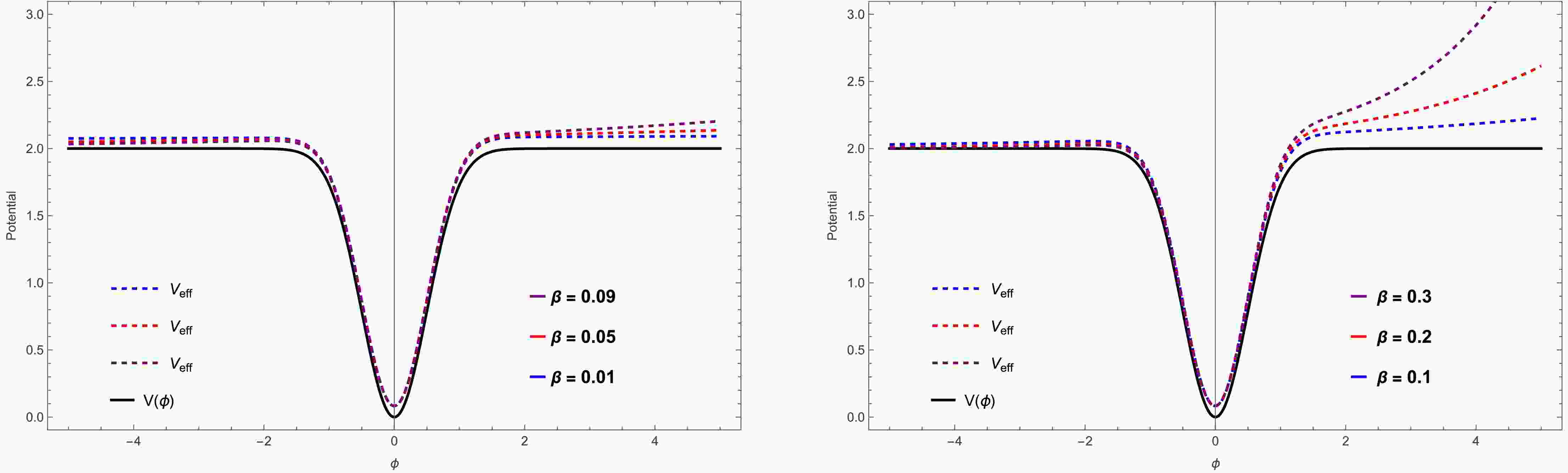
We begin our analysis by considering an exponential dependence of the neutrino mass on the scalar field, $ m_{\nu}(\phi)=m_0 e^{\beta \phi} $, which represents one of the simplest and most widely studied realizations of mass-varying neutrino (MaVaN) models. In this case, the coupling between the neutrino sector and the scalar field modifies the inflaton dynamics through a β-dependent correction to the effective potential.

In Fig. 1, we compare the bare scalar potential $ V(\phi) $ with the effective potential $ V_{\rm{eff}}(\phi) $ in the mass-varying neutrino (MaVaN) scenario with an exponential neutrino mass, for fixed parameters $ V_0 = 2 $ and $ \alpha = 2 $. The black solid curve represents the bare potential, while the colored dashed curves correspond to the effective potential for different values of the coupling parameter β. For small coupling strengths, $ V_{\rm{eff}}(\phi) $ closely follows the bare potential, indicating that neutrino back reaction term 39 is negligible. As β increases, the effective potential becomes progressively shallower around its minimum and exhibits a steeper rise at large positive field values, reflecting the growing contribution of the neutrino sector to the total energy density. For sufficiently large values of β, as shown in the right panel of Fig. 1, the effective potential increases rapidly for positive ϕ, while for negative ϕ it closely follows the standard scalar potential. This deformation modifies both the slope and curvature of the inflationary potential, thereby influencing the slow-roll dynamics and the resulting inflationary observables. The figure clearly demonstrates that the coupling parameter β plays a crucial role in shaping the effective potential and controlling the impact of neutrino mass variation on inflationary evolution.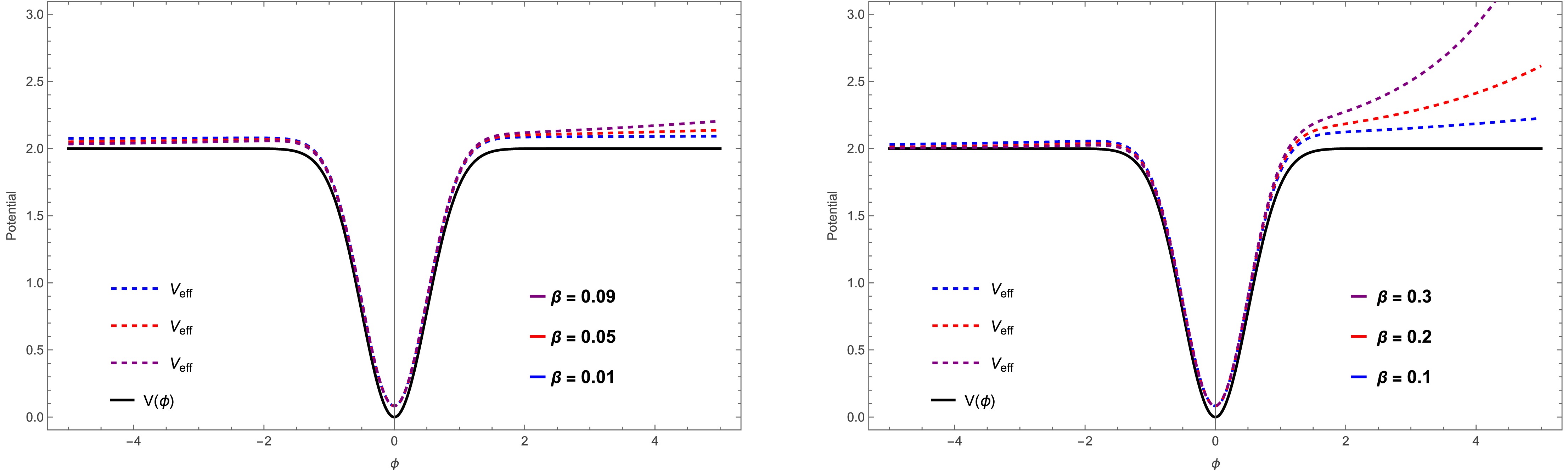

Figure 1.  (color online) Comparison of the bare potential $ V(\phi) $ and the effective potential $ V_{{\rm{eff}}}(\phi) $ for a MaVaN mass $ m_{\nu}(\phi)=m_0e^{\beta \phi} $ where $ m_0=1 $ in appropriate units. The plot shows the effect of the coupling parameter β for fixed $ V_0=2 $, $ \alpha=2 $.

To quantify the impact of the MaVaN mass variation on the inflationary dynamics, we evaluate the slow-roll parameters derived from the effective potential. These parameters characterize the validity of the slow-roll regime and form the basis for computing the key inflationary observables, namely the scalar spectral index $ n_s $ and the tensor-to-scalar ratio r.

The slow-roll parameters are evaluated as,

The slow-roll parameters $ \epsilon $ and η are influenced by the coupling parameter β, which governs the effect of neutrino backreaction on the inflationary dynamics. For smaller β, the slow-roll conditions $ \epsilon \lt 1 $ and $ |\eta| \lt 1 $ remain satisfied, ensuring a prolonged inflationary phase.

Fig. 2 illustrates the time evolution of the first and second slow-roll parameters, $ \epsilon $ (left panel) and η (right panel), for the MaVaN inflationary scenario with fixed parameters $ V_0 = 2 $ and $ \alpha = 2.2 $, and for three representative values of the coupling parameter $ \beta = 0.1 $, $ 0.2 $, and $ 0.3 $. In both panels, the slow-roll parameters decrease rapidly at early times and subsequently approach small, nearly constant values, indicating a sustained slow-roll regime. The initial magnitudes of $ \epsilon $ and η increase slightly with increasing β, reflecting the enhanced contribution of the neutrino sector to the effective potential. However, for all coupling values considered, both parameters remain well below unity throughout the evolution, ensuring the validity of the slow-roll approximation and the occurrence of successful inflation. This behavior demonstrates that while the neutrino–scalar coupling modifies the early-time dynamics, it does not spoil the slow-roll conditions for the parameter ranges explored.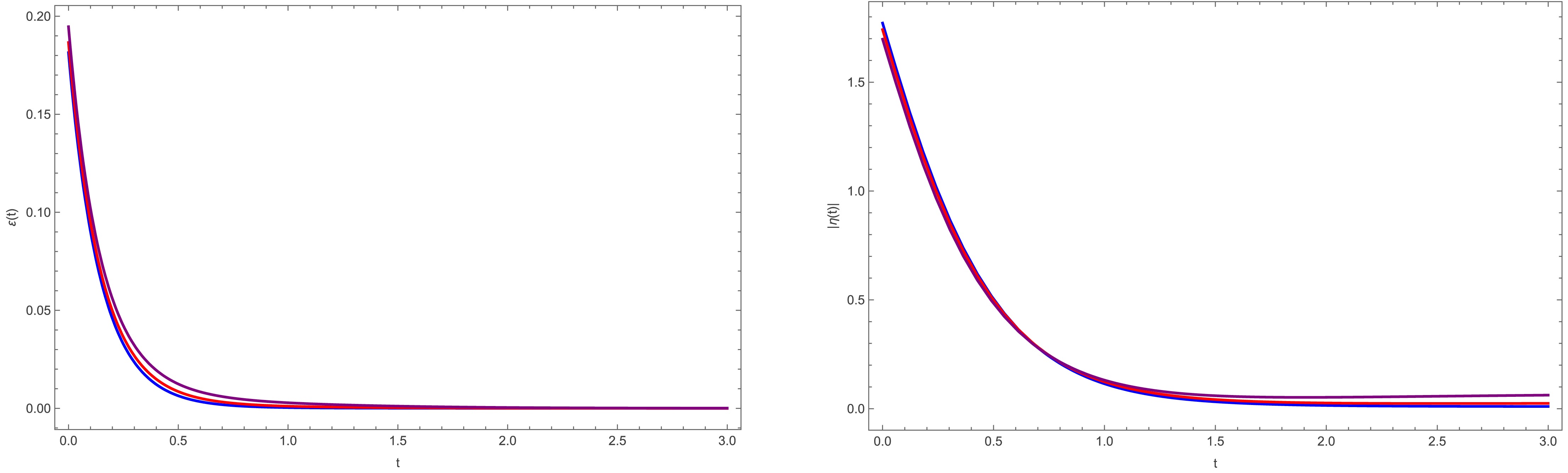

Figure 2.  (color online) Evolution of the first (left panel) and second (right panel) slow-roll parameters, $ \epsilon $ and η, respectively, for the exponential MaVaN mass model with $ V_0 = 2 $ and $ \alpha = 2 $. The blue, red, and purple curves correspond to the coupling parameters $ \beta = 0.1 $, $ \beta = 0.2 $, and $ \beta = 0.3 $, respectively.

The Spectral index $ n_s $ and scalar-to-tensor ratio are evaluated as,

Fig. 3 illustrates the plot of inflationary observables $ n_s $ vs. β and r vs. β for assumed values of $ V_0 = 2 $ and $ \alpha = 2.2 $. The left panel shows that the allowed values of coupling parameter β are constrained through observational upper and lower limit of $ n_s $. As the coupling strength increases, the curvature of the effective potential is enhanced, leading to a monotonic decrease in $ n_s $. The horizontal dashed lines indicate the Planck observational bounds, $ 0.9607 \lt n_s \lt 0.9691 $, which restrict the allowed range of the coupling parameter to $ 0.243 \lt \beta \lt 0.312 $. The right panel depicts the tensor-to-scalar ratio r vs. β, exhibiting a rapid growth of r for larger coupling values due to the corresponding increase in the slow-roll parameter $ \epsilon $. The dotted and dashed horizontal lines denote the observational upper limits $ r \lt 0.1 $ and $ r \simeq 0.065 $, respectively, yielding the allowed range $ 0.661 \lt \beta \lt 0.730 $. Notably, within the parameter space explored, we find no overlapping range of the coupling parameter β for which both the scalar spectral index $ n_s $ and the tensor-to-scalar ratio r simultaneously satisfy the current observational bounds. This result highlights the strong sensitivity of inflationary observables to neutrino mass variation and suggests that consistency with observations may be achieved for alternative choices of the initial parameters $ V_0 $ and α.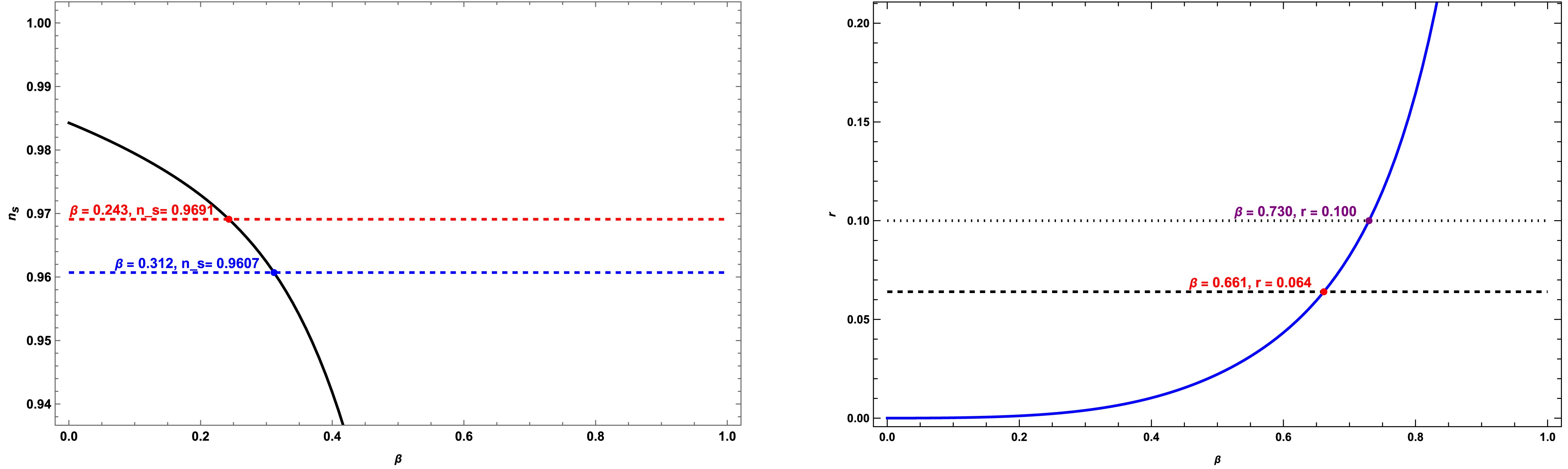

Figure 3.  (color online) Left panel: Plot of spectral index $ n_s $ vs. β parameter with $ V_0=2 $ and $ \alpha=2.2 $ for $ m_{\nu}(\phi)=m_0e^{\beta \phi} $ where $ m_0=1 $. The above dashed red straight lines shows the observational upper limit of $ n_s= 0.9691 $ and the straight dashed blue line is lower limit of $ n_s=0.9607 $. The value of coupling parameter β must lie between $ 0.243< \beta \lt 0.312 $. Right panel: Represents the plot between tensor-to-scalar ratio r vs β parameter. The dotted straight line represent upper limit with $ r<0.1 $ and the other observational limit with dashed straight line $ 0.065 $. The observational constraints on the coupling parameter β are $ 0.661<\beta<0.730 $.

It is interesting to further examine the correlation between the tensor-to-scalar ratio r and the scalar spectral index $ n_s $ by plotting r versus $ n_s $ for fixed values of the coupling parameter β. Fig. 4 illustrates this correlation for the exponential MaVaN scenario, highlighting how the inflationary observables evolve for fixed β. The purple and red curves correspond to $ \beta = 0.980 $ and $ \beta = 0.975 $, respectively, with parameters fixed at $ V_0 = 2 $ and $ \alpha = 4 $. As the scalar field evolves during inflation, the model traces trajectories in the $ (n_s,r) $ plane, reflecting the underlying slow-roll dynamics governed by the effective potential. The horizontal observational bounds on the tensor-to-scalar ratio are indicated, and the black dots mark the intersection points of the model predictions with these limits, explicitly identifying the corresponding values of $ (n_s,r) $. For $ \beta = 0.980 $, the intersections occur at $ (n_s,r) = (0.9185,0.065) $ and $ (n_s,r) = (0.9804,0.100) $, while for $ \beta = 0.975 $ they occur at $ (n_s,r) = (0.9335,0.065) $ and $ (n_s,r) = (0.9927,0.100) $. For these values of β, the observationally allowed range of $ n_s $ is consistent with the tensor-to-scalar constraint $ r \lt 0.1 $. This behavior highlights the strong sensitivity of the joint $ (n_s,r) $ predictions to the neutrino-scalar coupling and demonstrates how combined observational constraints can be employed to delineate viable regions of parameter space in the MaVaN framework.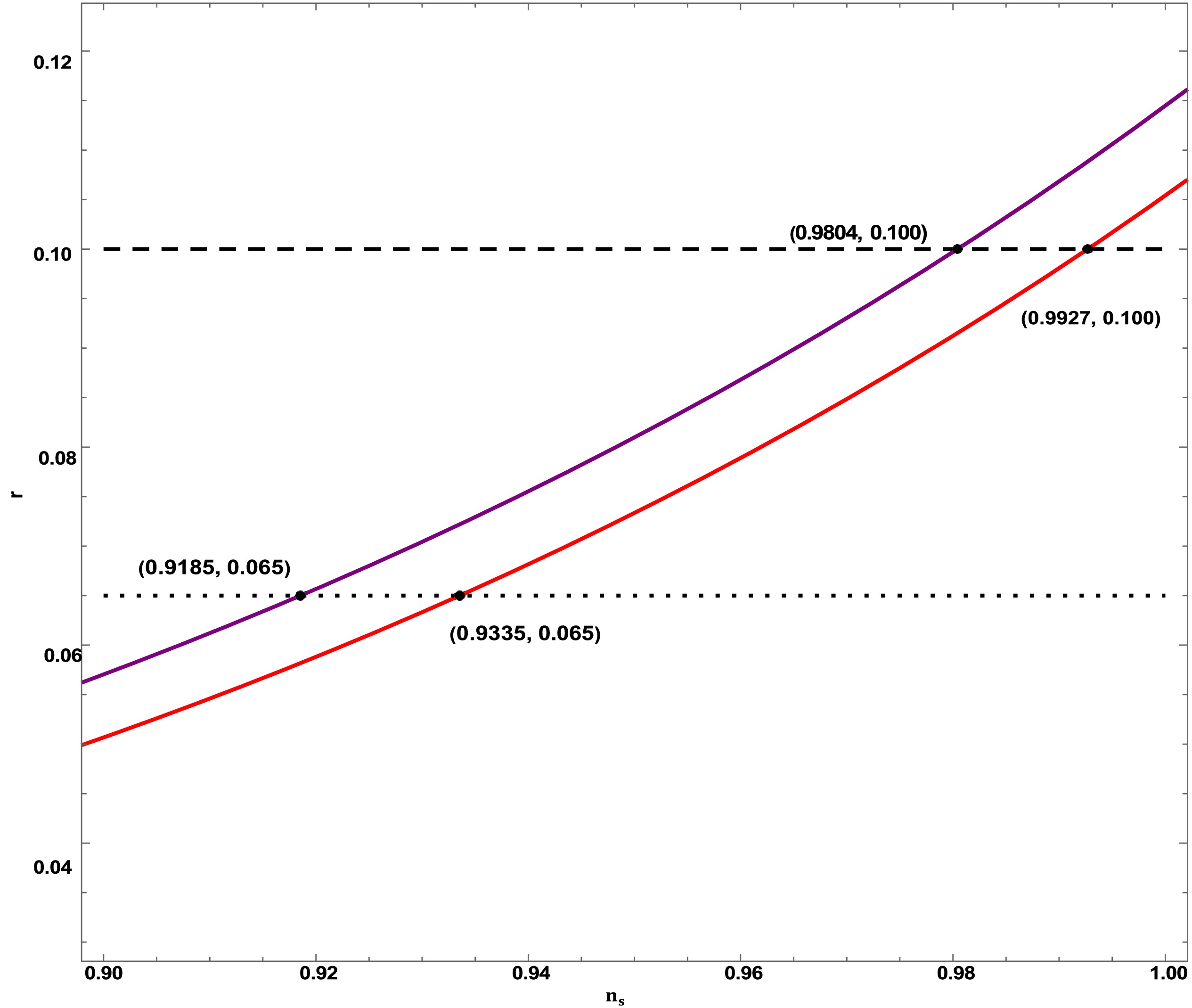

Figure 4.  (color online) Plot between tensor-to-scalar ratio r vs spectral index $ n_s $ for exponential MaVaN for two values of coupling parameter β the purple line for $ \beta=0.980 $ and red line for $ \beta=0.975 $. We assume $ V_0=2 $ and $ \alpha=4 $. The points of intersection are shown with black dot with values $ (n_s,r)=(0.9185,0.065),(0.9804,0.100) $ for $ \beta=0.980 $ and $ (n_s,r)=(0.9335,0.065),(0.9927,0.100) $ for $ \beta=0.975 $

We now examine the quantitative behaviour of the effective mass. For a Gaussian-type scalar potential and an exponentially varying neutrino mass, $ m_{\nu}(\phi)=m_0 e^{\beta \phi} $, the effective potential is given by

where $\widetilde{\rho}_{\nu} = \rho_{\nu} e^{-\beta \phi} $ and $\widetilde{p}_{\nu} = p_{\nu} e^{-\beta \phi} $ are independent of ϕ ^[33]. In the regime $ \alpha \phi^2 \gg 1 $, the minimum of the effective potential is located at

assuming $ \alpha>0 $ and $ \beta>0 $. The effective mass of the scalar field is defined as

which yields

This expression shows that the coupling between the scalar field and mass-varying neutrinos can induce a negative (tachyonic) contribution to the effective mass. In particular, for positive α, β, $ V_0 $, and $ (\rho_{\nu} - 3p_{\nu}) $, the effective mass squared becomes negative when

indicating an instability in the scalar sector driven by the neutrino coupling.

For a power-law neutrino mass of the form $ m_{\nu}(\phi)= m_0 \phi^n $, we show the comparison plot of the scalar field potential $ V(\phi) $ and the effective potential $ V_{{\rm{eff}}}(\phi) $ for different values of the coupling parameter n. The black solid curve represents the original potential $ V(\phi) $, which exhibits a symmetric shape with a well-defined minimum at $ \phi = 0 $. The colored dashed curves correspond to the effective potential $ V_{{\rm{eff}}}(\phi) $. It is evident that the inclusion of the coupling between the scalar field and neutrinos significantly modifies the potential away from the minimum. For small values of the coupling parameter n, the effective potential closely follows the bare potential near the minimum, indicating that neutrino backreaction is weak in this regime. However, as n increases, the effective potential becomes progressively steeper and rises more rapidly for large values of $ |\phi| $, reflecting the increasing contribution of the neutrino sector to the total energy density. In particular, for larger values of n, the deviations of $ V_{{\rm{eff}}}(\phi) $ from $ V(\phi) $ become more pronounced at large field values, demonstrating that stronger power-law coupling enhances the sensitivity of the effective potential to the scalar field.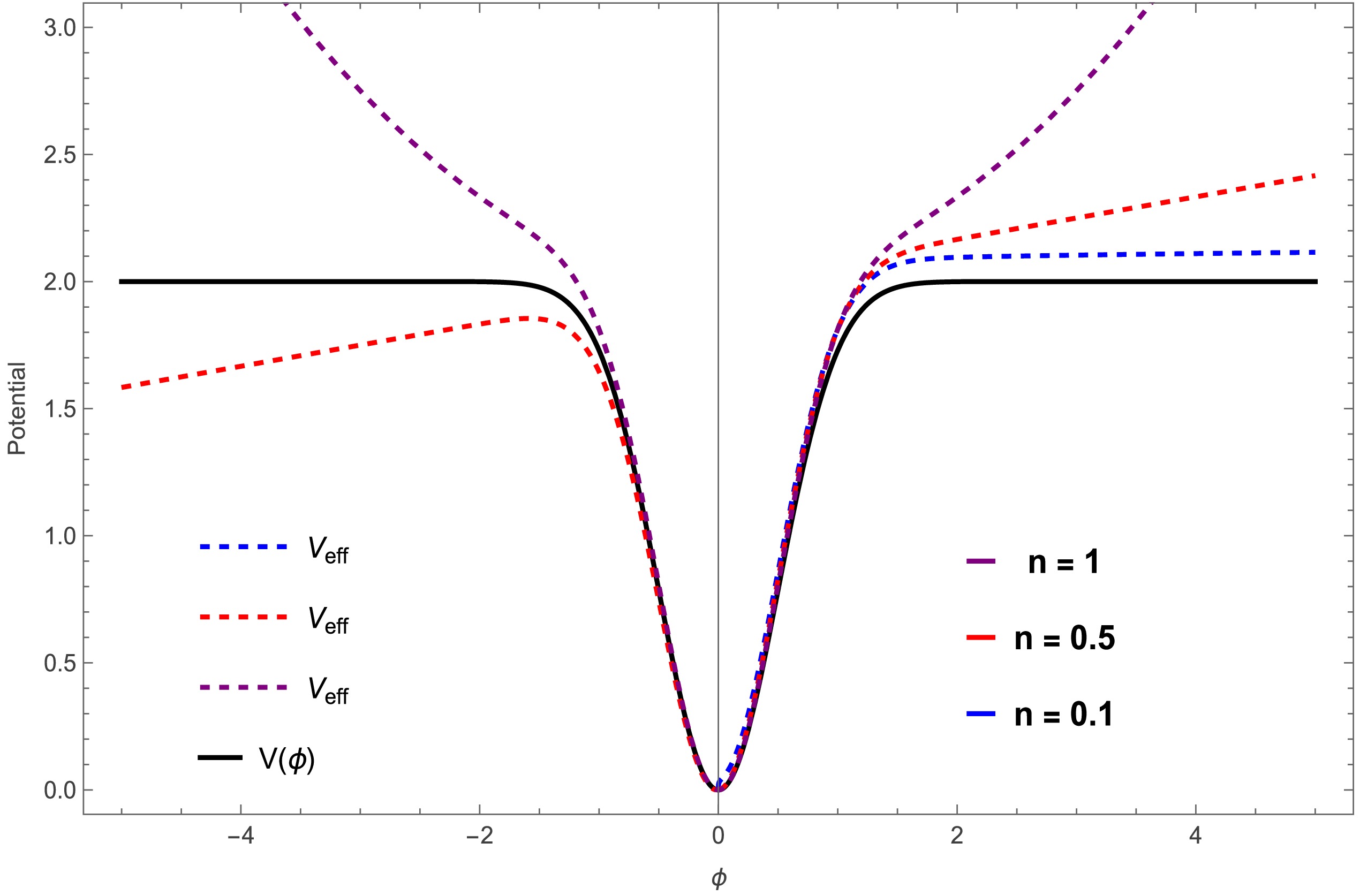

Figure 5.  (color online) Comparison of $ V(\phi) $ and $ V_{\rm{eff}}(\phi) $ for a power-law MaVaN mass $ m_{\nu}(\phi)=m_0\phi^n $ with $ m_0=1 $, for different values of n and fixed $ V_0=2 $, $ \alpha=2 $.

The neutrino–scalar coupling deforms the effective potential by modifying its slope and curvature, thereby affecting the inflationary dynamics. We therefore evaluate the slow-roll parameters, which determine the scalar spectral index $ n_s $ and the tensor-to-scalar ratio r.The slow-roll parameters are evaluated as,

Fig. 6 illustrates the time evolution of the first (left panel) and second (right panel) slow-roll parameters, $ \epsilon(t) $ and $ \eta(t) $, respectively, for the power-law MaVaN scenario with $ V_0 = 2 $ and $ \alpha = 2 $. The blue, red, and purple curves correspond to the coupling parameters $ n = 0.1 $, $ n = 0.5 $, and $ n = 1 $, respectively. The left panel shows that the first slow-roll parameter $ \epsilon $ decreases rapidly with time for all values of n and remains well below unity throughout the evolution, indicating that the slow-roll condition is satisfied and inflation proceeds consistently in this regime. Increasing the coupling parameter n slightly delays the decay of $ \epsilon $, reflecting a mild enhancement of the effective potential slope due to the neutrino coupling.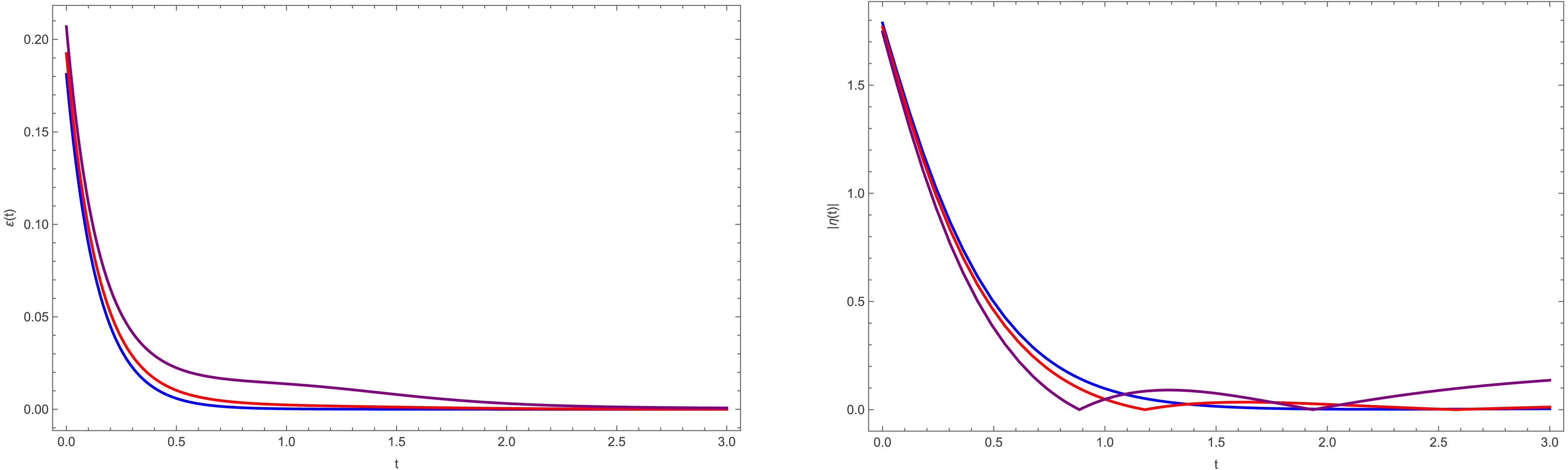

Figure 6.  (color online) Evolution of the first (left panel) and second (right panel) slow-roll parameters, $ \epsilon $ and η, respectively, for the power law MaVaN mass model with $ V_0 = 2 $ and $ \alpha = 2 $. The blue, red, and purple curves correspond to the coupling parameters $ n = 0.1 $, $ n = 0.5 $, and $ n = 1 $, respectively.

The right panel displays the evolution of the second slow-roll parameter η, which exhibits a more sensitive dependence on the coupling parameter. While η initially decreases in magnitude for all cases, larger values of n lead to more pronounced deviations and mild oscillatory behavior at later times. Nevertheless, $ |\eta| $ remains sufficiently small during the relevant inflationary phase, ensuring the validity of the slow-roll approximation. The transient oscillations observed for larger n originate from the increased curvature of the effective potential induced by the power-law neutrino mass coupling. Overall, Fig. 6 demonstrates that the power-law MaVaN coupling modifies the detailed evolution of the slow-roll parameters without spoiling the inflationary dynamics.For large value of coupling term n enhances the sensitivity of $ \epsilon $ and η to the scalar field evolution, but the slow-roll conditions remain intact, confirming the consistency of the inflationary scenario within the explored parameter range.

The Spectral index $ n_s $ and Scalar-to-tensor ratio r are,

In Fig. 7, we plot the spectral index $ n_s $ and tensor-to-scalar ratio r w.r.t. the parametric space of the coupling parameter n for power law MaVaN scenario with the initial parameter $ V_0=2 $ and $ \alpha=1.9 $. The left panel shows the variation of the scalar spectral index $ n_s $ with n, where the solid curve exhibits a monotonic increase in $ n_s $. The red and blue dashed horizontal lines indicate the Planck observational bounds $ n_s = 0.9691 $ and $ n_s = 0.9607 $, respectively, which constrain the coupling parameter to the narrow range $ 0.300 \lt n \lt 0.352 $. The right panel depicts the tensor-to-scalar ratio r versus n, demonstrating a rapid growth of r with increasing coupling strength. The dotted and dashed horizontal lines correspond to the observational upper limits $ r \lt 0.1 $ and $ r \simeq 0.065 $, yielding the allowed range $ 0.755 \lt n \lt 0.891 $. Similar to the exponential case, within the parameter space explored, we find no overlapping range of the coupling parameter n for which both $ n_s $ and r simultaneously satisfy the current observational bounds. This strong sensitivity suggest to probe the inflationary observables for alternative choices of the initial parameters $ V_0 $ and α.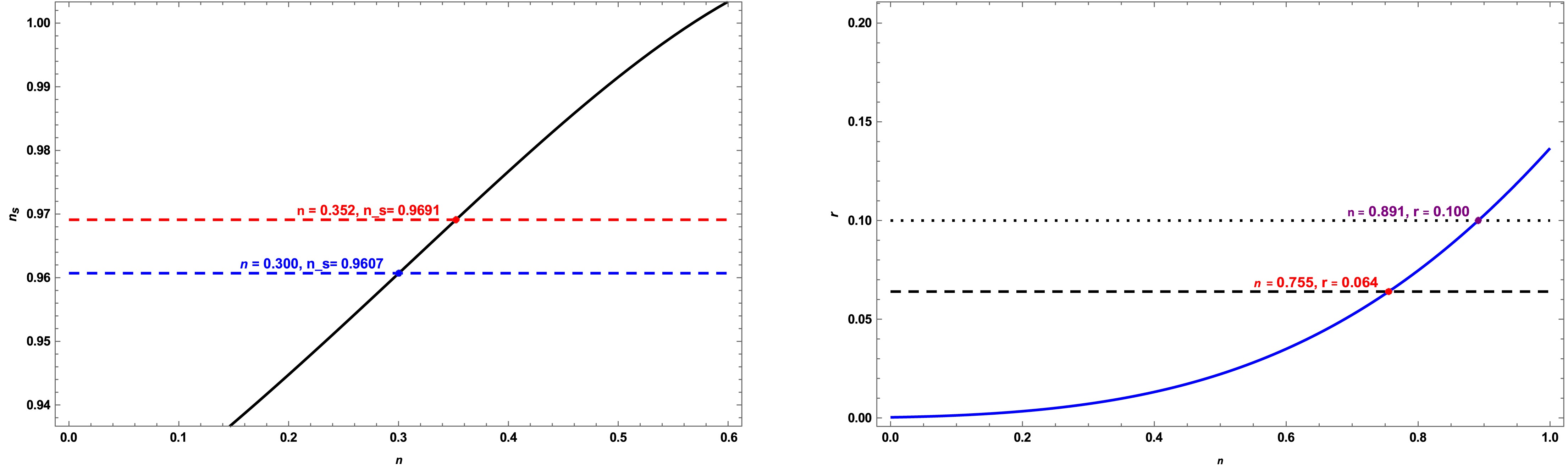

Figure 7.  (color online) Left panel: Plot of spectral index $ n_s $ vs. n parameter with $ V_0=2 $ and $ \alpha=1.9 $ for $ m_{\nu}(\phi)=m_0\phi^n $, where $ m_0=1 $. The above dashed red straight lines shows the observational upper limit of $ n_s= 0.9691 $ and the straight dashed blue line is lower limit of $ n_s=0.9607 $. The value of coupling parameter n must lie between $ 0.300< n \lt 0.352 $. Right panel: Represents the plot between tensor-to-scalar ratio r vs n parameter. The dotted straight line represent upper limit with $ r<0.1 $ and the other observational limit with dashed straight line $ 0.065 $. The observational constraints on the coupling parameter β are $ 0.755<n<0.891 $.

Fig. 8 presents the plot between the tensor-to-scalar ratio r and the scalar spectral index $ n_s $ for assumed initial values $ V_0=2 $ and $ \alpha=2.5 $. The red and blue curves correspond to the coupling parameters $ n=0.99 $ and $ n=1.2 $, respectively. As inflation proceeds, the evolution of the scalar field traces trajectories in the $ (n_s,r) $ plane, reflecting the slow-roll dynamics governed by the effective potential modified by the neutrino coupling. The horizontal dashed lines indicate the observational upper bounds, namely $ r\simeq0.065 $ and $ r<0.1 $.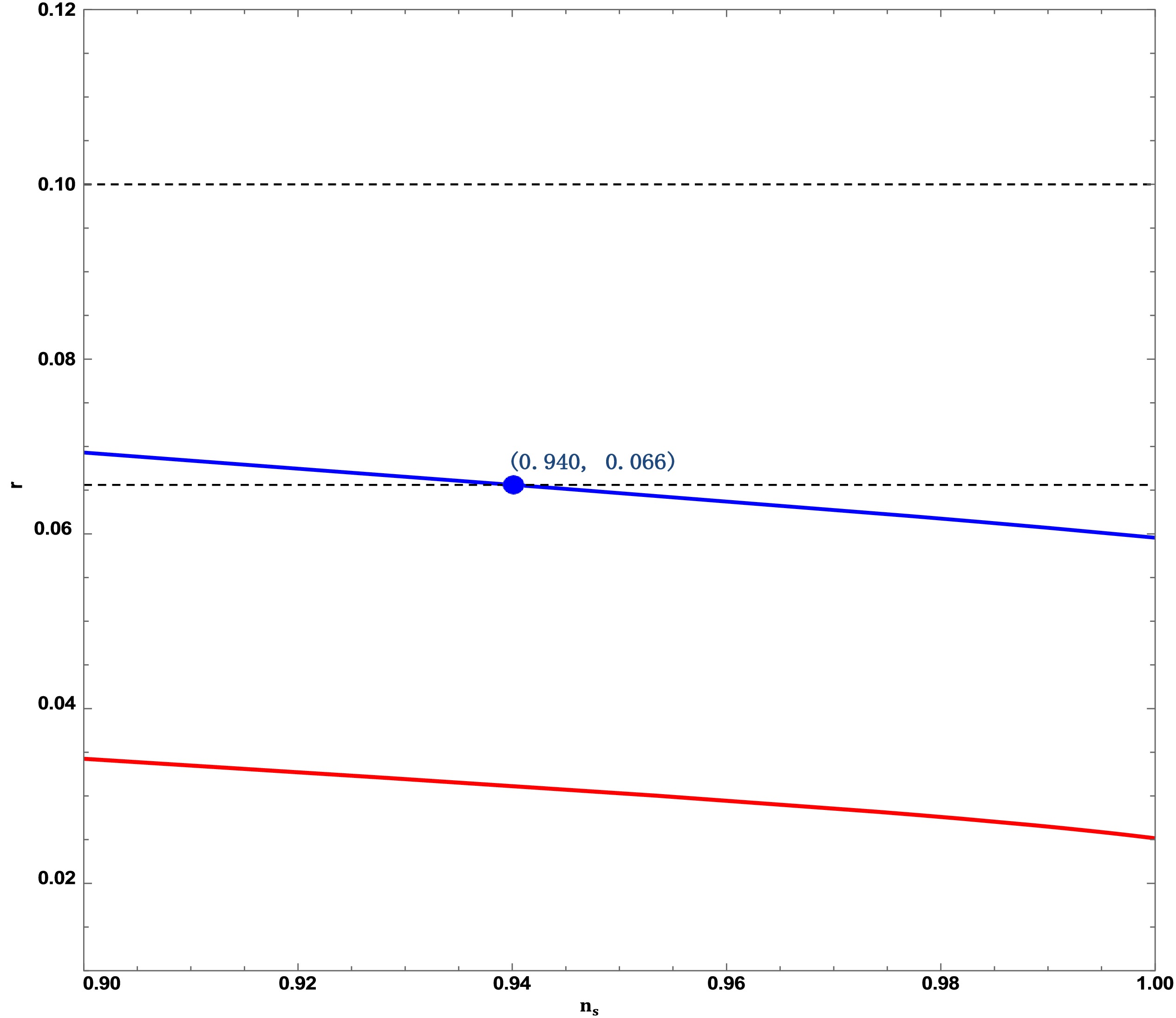

Figure 8.  (color online) Plot between tensor-to-scalar ratio r vs spectral index $ n_s $ for power law mass of MaVaN for two values of coupling parameter n, the red line for $ n=0.99 $ and the blue line for $ n=1.2 $. We assume $ V_0=2 $ and $ \alpha=2.5 $. The only intersection point is $ (n_s,r)=(0.940,0.66) $ for $ n=1.2 $.

For smaller values of the coupling parameter $ n<1 $, the r remains highly suppressed throughout the evolution, and the corresponding trajectories do not intersect the observational bounds. In this regime, r stays well below the observational limits for values of $ n_s $ within the observationally allowed range, indicating that tensor-mode production is negligible. In contrast, for larger values of the coupling parameter $ n>1 $, as exemplified by $ n=1.2 $, the tensor-to-scalar ratio increases significantly and intersects the observational bound at a single point. This intersection occurs at $ (n_s,r)=(0.940,0.066) $, marking the only configuration in this parameter set where the model predictions marginally satisfy the tensor constraint. For this case, consistency with observations on $ n_s $ is satisfy for the range $ r\lesssim0.065 $. These results demonstrate that the power-law neutrino–scalar coupling plays a crucial role in shaping the inflationary predictions. While smaller values of n lead to suppressed tensor modes and broad compatibility with observations, larger values of n enhance tensor-mode production and severely restrict the allowed region of parameter space.

For a Gaussian-type scalar potential and a power-law varying neutrino mass, $ m_{\nu}(\phi)=m_0 \phi^n $, the effective potential develops a minimum in the regime $ \alpha \phi^2 \gg 1 $. The location of the minimum is given by

assuming α > 0 and $ n>0 $. The effective mass of the scalar field, defined as $m_{\rm{eff}}^2 = \left. \partial^2 V_{\rm{eff}}/\partial \phi^2 \right|_{\phi=\phi_{\min}},$ takes the form

This result indicates that the coupling between the scalar field and mass-varying neutrinos can generate a negative (tachyonic) contribution to the effective mass. In particular, for $ n>1 $ and positive α, $ V_0 $, and $ (\rho_{\nu} - 3p_{\nu}) $, the effective mass squared becomes negative when

signalling an instability in the scalar sector induced by the neutrino coupling. In contrast, for $ 0<n<1 $, the effective mass remains positive for positive values of α and $ V_0 $, ensuring stability of the scalar field in this regime.

For the mixed MaVaN mass scenario, we present in Fig. 9 a comparison between the standard scalar potential in the absence of neutrino coupling and the corresponding effective potential. The left and right panels correspond to the coupling parameters $ n=0.1 $ and $ n=0.5 $, respectively. The solid black curve represents the Gaussian-type scalar potential $ V(\phi) $, which is symmetric and possesses a well-defined minimum at $ \phi=0 $. For $ n=0.1 $, the effective potential $ V_{\rm{eff}}(\phi) $ is shown for different values of the coupling parameter β. As β increases, the deviation of the effective potential from the bare potential becomes increasingly pronounced for large positive values of the scalar field, indicating a growing contribution from the neutrino sector. For value of $ n=0.5 $, a qualitatively similar behavior is observed for large positive field values, where the effective potential deviates more strongly from the bare potential as β increases. However, in this case, the effective potential lies below the standard potential for negative values of the scalar field, indicating a stronger asymmetry induced by the mixed neutrino mass coupling.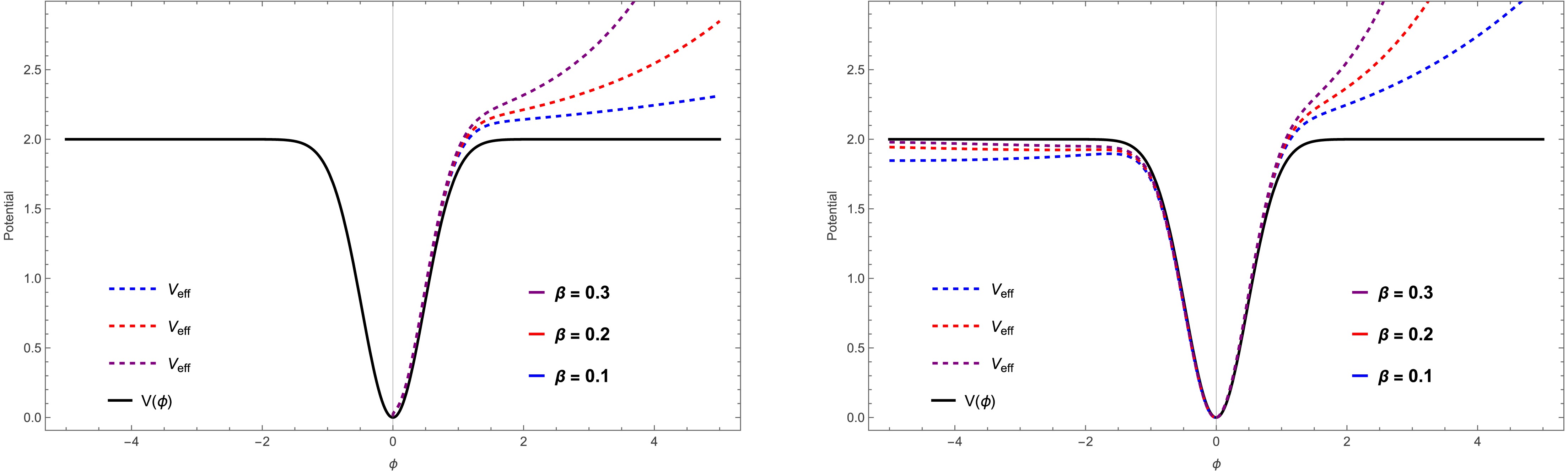

Figure 9.  (color online) Comparison of the bare potential $ V(\phi) $ and the effective potential $ V_{{\rm{eff}}}(\phi) $ for a MaVaNa mass $ m_{\nu}(\phi)=m_0\phi^n e^{\beta \phi} $ for $ m_0=1 $.Left Plot: Shows the effect of the coupling parameter β and the power n for fixed $ V_0=2 $, $ \alpha=2.2 $ for $ n=0.1 $. Right Plot: illustrates the effect of for fixed $ V_0=2 $, $ \alpha=2.2 $ for $ n=0.5 $.

The neutrino-scalar coupling deforms the effective potential by modifying its slope and curvature, thereby affecting the inflationary dynamics. We therefore evaluate the slow-roll parameters, which determine the scalar spectral index $ n_s $ and the tensor-to-scalar ratio r. The slow-roll parameters are evaluated as

The Spectral index $ n_s $ and Scalar-to-tensor ratio r are calculated,

The mixed coupling form generalizes the previous two cases, with the parameters β and n jointly determining the strength and nature of the scalar–neutrino interaction. While β governs the exponential sensitivity of $ m_{\nu}(\phi) $ to the scalar field, the power-law index n introduces an additional field-dependent modulation. As a result, the effective potentials slope and curvature, represented by the slow-roll parameters $ \epsilon $ and η, exhibit a richer dynamical behaviour, allowing for a broader range of inflationary and post-inflationary evolutions compared to the purely exponential or power-law couplings.

Fig. 10 depicts the time evolution of the slow-roll parameters $ \epsilon $ and η for values assumed $ V_0 = 2 $ and $ \alpha = 2 $, with a fixed power index $ n = 0.5 $ and different values of the coupling parameter β. The blue, red, and purple curves correspond to $ \beta = 0.1 $, $ \beta = 0.2 $, and $ \beta = 0.3 $, respectively. From the left panel, it is evident that the slow-roll parameter $ \epsilon $ rapidly decreases with time and quickly approaches values much smaller than $ 1 $ for considered values of β. This confirms that the inflationary dynamics enter and remain within the slow-roll regime for different coupling strengths. The right panel illustrates the evolution of η, which initially exhibits relatively large values and then gradually decreases and remains less than 1, indicating the validity of the slow roll approximation and successful inflation.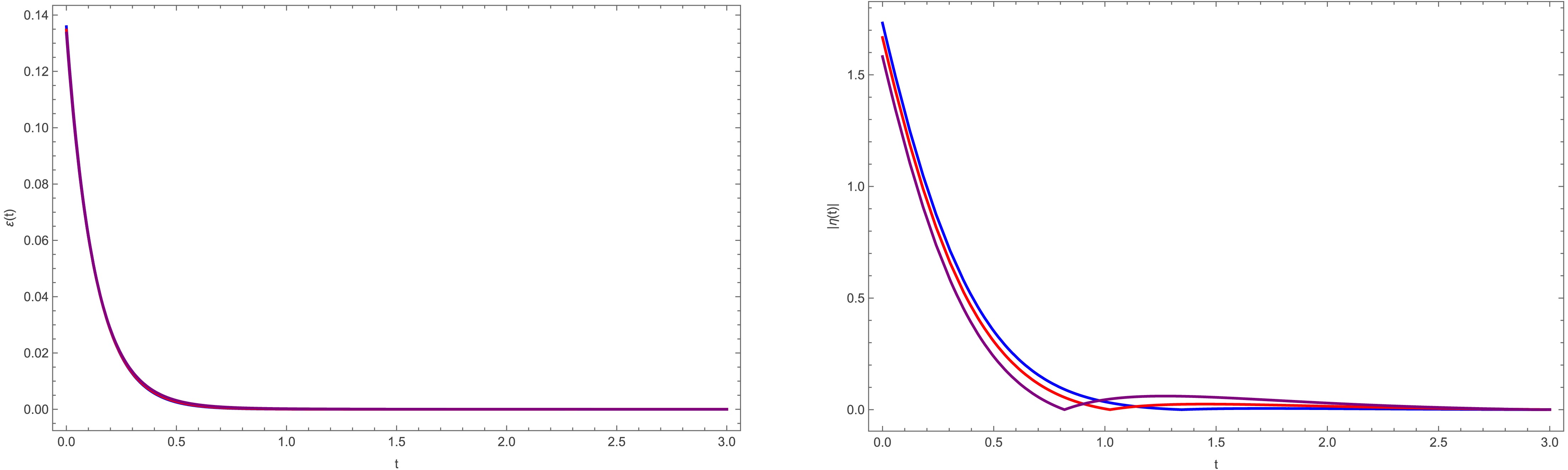

Figure 10.  (color online) Evolution of the first (left panel) and second (right panel) slow-roll parameters, $ \epsilon $ and η, respectively, for the mixed form of MaVaN mass model with $ V_0 = 2 $ and $ \alpha = 2 $. The blue, red, and purple curves correspond to the coupling parameters $ \beta = 0.1 $, $ \beta = 0.2 $, and $ \beta = 0.2 $, respectively, with $ n = 0.5 $.

In Fig. 11, we present the inflationary observables $ n_s $ and r for the parametric space of parameter β for the mixed MaVaN scenario, considering two representative values of $ n=0.2 $ (red curve) and $ n=0.0001 $ (orange curve). The left panel shows the ranges of β that satisfy the observational upper and lower bounds on the scalar spectral index $ n_s $. These ranges are found to be $ 0.06 \lt \beta \lt 0.14 $ for $ n=0.2 $ and $ 0.23 \lt \beta \lt 0.27 $ for $ n=0.0001 $. The right panel displays the corresponding constraints from the tensor-to-scalar ratio r, yielding the allowed intervals $ 0.38 \lt \beta \lt 0.44 $ for $ n=0.2 $ and $ 0.48 \lt \beta \lt 0.54 $ for $ n=0.0001 $. Notably, there is no overlapping range for the coupling parameter β that satisfies the current observational constraints on both $ n_s $ and r.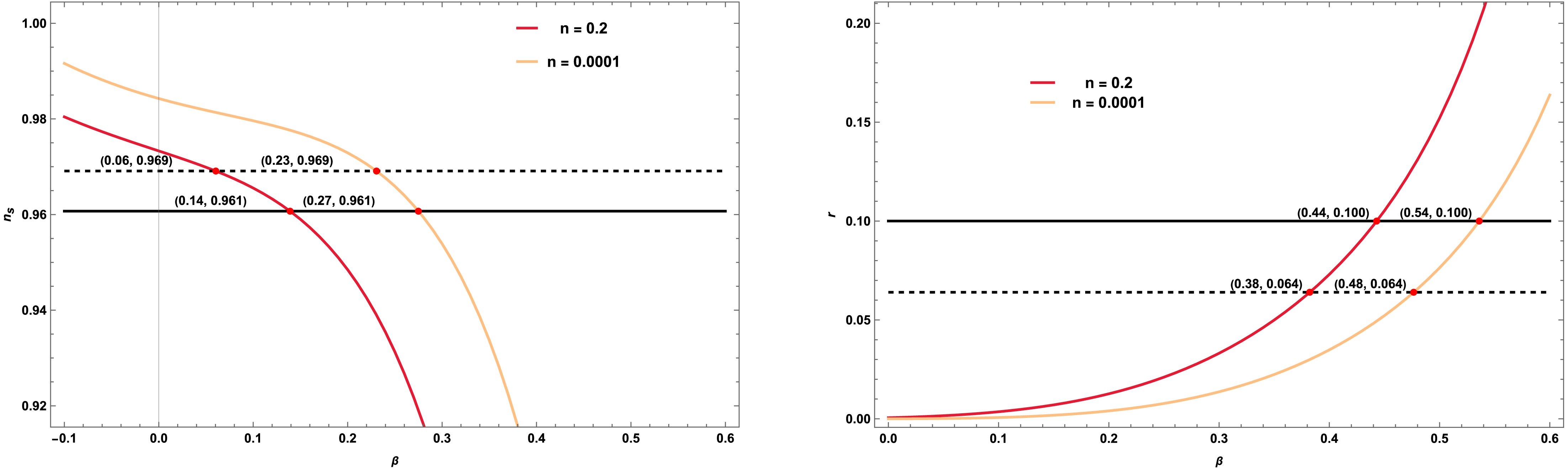

Figure 11.  (color online) Left panel: Plot of spectral index $ n_s $ vs. β parameter for the mixed MaVaN scenario with $ V_0 = 2 $ and $ \alpha = 2.2 $. The above dashed straight lines shows the observatioanl upper limit of $ n_s= 0.09691 $ and the straght dark line is lower limit of $ n_s=0.9607 $. For assumed value of $ n=0.2 $ and $ n=0.0001 $ the value of coupling parameter β must lie between $ 0.06 \lt \beta \lt 0.14 $ and $ 0.23< \beta \lt 0.27 $, respectively. Right panel: Represents the plot between tensor-to-scalar ratio r vs β parameter. The upper limit black straight line with $ r<0.1 $ and the other observational limit with dashed straight line $ 0.065 $. The observational constraints on the coupling parameter β are $ 0.38<\beta<0.44 $ and $ 0.48<\beta<0.54 $, respectively.

To investigate the inflationary predictions of the MaVaN framework, we numerically solve the coupled background equations governing the evolution of the scalar field and the scale factor in the presence of a modified effective potential. For fixed values of the potential parameters $ V_0 $ and α, we perform a systematic scan over the coupling parameter β for selected values of n in Fig. 12. This procedure generates continuous trajectories in the $ (n_s,r) $ plane as the coupling parameter β is varied. To confront the model with current cosmological observations, we superimpose the observational bounds on the tensor-to-scalar ratio, $ r<0.1 $ and $ r\simeq0.065 $. A robust procedure is employed to identify the intersection points between the model trajectories and the observational bounds, thereby determining the corresponding values of $ (n_s,r,\beta) $ that are consistent with the data.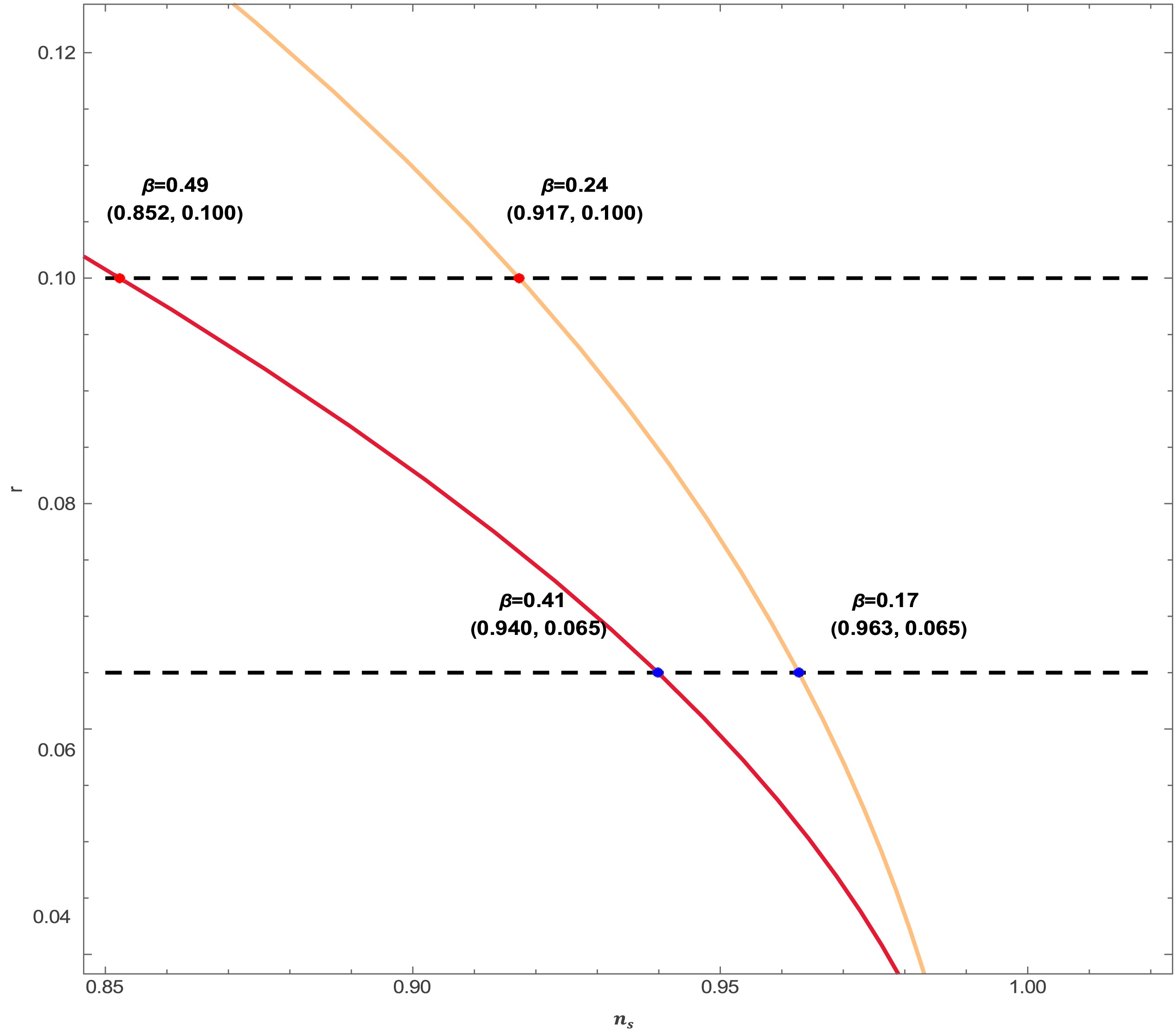

Figure 12.  (color online) Plot between tensor-to-scalar ratio r vs spectral index $ n_s $ for mixed form MaVaN for two values of n, the red line for $ n=0.2 $ and orange line for $ n=0.7 $. We assume $ V_0=2 $ and $ \alpha=2.5 $. The points of intersection are shown with blue and red dots with values $ (n_s,r,\beta)=(0.852,0.100,0.49),(0.940,0.065,0.41) $ for $ n=0.2 $ and $ (n_s,r,\beta)=(0.917,0.100,0.24),(0.963,0.065,0.17) $ for $ n=0.7 $

From Fig. 12, we find that only a very limited region of parameter space satisfies the observational constraints. In particular, for $ n=0.7 $, the trajectory intersects the observational bound at $ \beta \simeq 0.17 $, yielding $ (n_s,r) \simeq (0.963,0.065) $, which lies within the observationally allowed range of the scalar spectral index.

For mixed form of the neutrino mass,$ m_{\nu}(\phi) = m_0 \phi^n e^{\beta \phi} $, combining power-law and exponential dependence. The corresponding effective potential can be written as

where $ (\rho_{\nu} - 3p_{\nu}) $ does not depend on ϕ. In the regime $ \alpha \phi^2 \gg 1 $, the minimum of the effective potential is determined by the extremization condition $ \frac{dV_{\rm{eff}}}{d\phi}=0 $, which yields

where $ {\cal{P}}=\rho_{\nu} - 3p_{\nu} $. One can obtain the $ \phi_{{\rm{min}}} $ for exponential and power law cases by choosing $ n=0 $ and $ \beta=0 $, respectively. The effective mass of the scalar field obtained at $ \phi_{{\rm{min}}} $ is

Equation (59) shows that the simultaneous power-law and exponential coupling between the scalar field and mass-varying neutrinos can significantly modify the effective mass. Depending on the parameters $ (n,\beta) $ and the background neutrino density, the effective mass squared may acquire a negative (tachyonic) contribution, providing a possible instability of the scalar sector. In appropriate limits, Eq. (59) smoothly reduces to the pure power-law and pure exponential cases discussed earlier.

In this work, we explore cosmological framework where neutrino masses arise dynamically through their coupling with a scalar field that also drives the inflationary expansion of the Universe. We begin with the Einstein–Hilbert action in a spatially flat FLRW spacetime, and derive the Friedmann and Raychaudhuri equations, in the presence of mass-varying neutrinos as a matter component. The modified continuity relations describe the energy exchange between the scalar field and the neutrino sector, illustrating how their interaction affects the overall dynamics. This coupling, introduced through the conformal function $ B(\phi) $, leads to a nontrivial evolution of the energy densities and thereby alters the standard cosmic expansion history. When the neutrino mass depends explicitly on the scalar field, the model naturally gives rise to a class of mass-varying neutrino (MaVaN) scenarios, providing a unified picture in which neutrino mass generation and cosmological evolution are deeply interconnected.

Neutrinos were treated as a collisionless and kinetically decoupled sector, whose phase-space distribution evolves according to the Liouville equation. Their energy density and pressure were derived from the general phase-space integrals, without assuming the existence of a thermal neutrino bath during inflation. In the relativistic regime relevant for inflation, the trace combination $ (\rho_{\nu} - 3p_{\nu}) $ is strongly suppressed and vanishes in the strictly massless limit. Nevertheless, this trace provides a parametrically small but nonzero contribution that enters the scalar-field dynamics through an effective potential $ V_{\rm{eff}}(\phi) $, encoding the back reaction of the neutrino sector on inflation.

We consider a Gaussian-type scalar potential and investigate three different form of the MaVaN mass namely, an exponential form, a power-law form, and a mixed power-law-exponential form. For each case, we derived the corresponding effective potential, evaluated the slow-roll parameters, and studied their time evolution to assess the consistency of the inflationary phase. We further computed the spectral index $ n_s $ and the tensor-to-scalar ratio r to constrain the coupling parameter through current observational bounds.

Our results demonstrate that all three classes of neutrino mass couplings considered in this work are capable of supporting a prolonged slow-roll inflationary phase for suitable choices of parameters. However, the inflationary observables exhibit a pronounced sensitivity to the neutrino–scalar coupling. In both the purely exponential and power-law cases, the observational constraints on the scalar spectral index $ n_s $ and the tensor-to-scalar ratio r restrict the coupling parameters to narrow and generally non-overlapping ranges. As a consequence, it is difficult to simultaneously satisfy all current observational bounds within these minimal realisations.

To further assess this behavior, we analysed the trajectories in the $ (n_s,r) $ plane for different values of the potential parameters $ V_0 $ and α. In the exponential mass case, for coupling values $ \beta = 0.980 $ and $ \beta = 0.975 $, the trajectories intersect the observational tensor bounds at $ (n_s,r) = (0.9185,0.065) $ and $ (0.9804,0.100) $ for $ \beta = 0.980 $, and at $ (0.9335,0.065) $ and $ (0.9927,0.100) $ for $ \beta = 0.975 $. For these values of β, the scalar spectral index can lie within the observationally allowed range while satisfying the tensor-to-scalar constraint $ r<0.1 $. In contrast, for the power-law mass form, the corresponding trajectories generally do not intersect the observational bounds. For coupling values $ n<1 $, the tensor-to-scalar ratio remains highly suppressed throughout the evolution, with r well below the observational limits for values of $ n_s $ within the allowed range, indicating negligible tensor-mode production. For larger coupling values $ n>1 $, as illustrated by the representative case $ n=1.2 $, the tensor-to-scalar ratio increases significantly and intersects the observational bound at a single point, $ (n_s,r)=(0.940,0.066) $. This point represents the only configuration in this parameter set where the tensor constraint is marginally satisfied, with consistency in $ n_s $ achieved only for $ r\lesssim 0.065 $. These features reflect the strong deformation of the effective potential induced by neutrino backreaction, which substantially alters both its slope and curvature.

The mixed power-law–exponential coupling introduces additional flexibility by combining the effects of both functional forms. The joint dependence on the parameters $ (n,\beta) $ leads to a richer phenomenology and allows for a limited region of observational viability. Our numerical analysis of the $ (n_s,r) $ trajectories reveals that only a narrow region of parameter space satisfies current observational constraints. In particular, for $ n\simeq 0.7 $, we find that the model simultaneously satisfies the bounds on $ n_s $ and r at $ \beta\simeq 0.17 $, yielding $ (n_s,r)\simeq (0.963,0.065) $. Outside this restricted region, the predictions typically fall outside the observationally allowed range.

We further analyzed the stability of the scalar sector by computing the effective mass at the minimum of the effective potential. In all three MaVaN forms, the neutrino–scalar coupling can induce negative (tachyonic) contributions to the effective mass for certain parameter choices, leading to potential instabilities. While such instabilities are absent in specific regions of parameter space, particularly for moderate coupling strengths, they place additional theoretical constraints on viable MaVaN inflationary models.

Overall, our results demonstrate that mass-varying neutrinos can play a nontrivial role in shaping the inflationary dynamics, even when their contribution is parametrically suppressed during the relativistic phase. At the same time, the strong sensitivity of inflationary observables to the neutrino-scalar coupling implies that current and future precision measurements of $ n_s $ and r provide a powerful probe of MaVaN scenarios. Extensions of this framework to alternative scalar potentials, different initial conditions, or post-inflationary epochs may further clarify the viability of neutrino-assisted inflation and its possible connections to late-time cosmology.