


 Abstract
 HTML
HTML Reference
 Related
 PDF
PDF


-
Understanding how the spins of fission products are formed is still a challenge in nuclear fission theory. This is particularly interesting when the spin of the parent nucleus is zero or very small, while the spins of the fission fragments (FFs) can reach values of up to six or seven
$ \hbar $ units. Currently, there are two candidate models [1, 2] that can explain this effect. However, both have limitations and drawbacks, which highlights the need for further research to develop a comprehensive and consistent model to accurately describe this phenomenon.The first model, proposed by Randrup et al. [3, 4], is based on the statistical model
$ \mathrm{FREYA} $ , which exploits the Monte Carlo method to determine the mass, charge, and velocity of primary fission fragments (PFFs). It follows the ideas reported in [5, 6], where the importance of nucleon exchange on the dynamical evolution of PFF spins was demonstrated. This exchange leads to the excitation of six rotational modes: transverse wriggling and bending modes (which are doubly degenerate), and longitudinal twisting and tilting modes. The mobility coefficients, which determine the time scales for these oscillations, were also estimated. Taking advantage of the results of this study on$ \mathrm{FREYA} $ , the realization of a complex mechanism of nucleon exchange assumes complete relaxation of transverse modes (wriggling and bending), while longitudinal modes (twisting and tilting) are not excited [7, 8].The second model, proposed by Bulgac et al. [1, 9, 10], is based on a microscopic approach using the time-dependent density functional theory (TDDFT), constructed by analogy with the derivation of Fermi's golden rule. Given that this model is based on general considerations, the analysis presented in related studies suggests that it is fundamentally rooted in the quantum angular momentum theory, with certain assumptions regarding the individual spin and angular momentum distributions. In the framework of this approach, contributions to the FF spins are considered not only from transverse bending and wriggling oscillations but also from longitudinal tilting and twisting oscillations, thus providing a description of spin in three-dimensional space. This is expected to impact, for example, the angular spin distributions and other key characteristics. The three-dimensional spin model presented in [10] differs significantly from the two-dimensional phenomenological model [11], where the spin is described in planes perpendicular to the Z-axis.
These two different model representations also have some similarities. For example, in [10], the importance of considering the FF moments of inertia was discussed, similar to [2], where it was pointed out that this quantity plays a key role in describing FF spin distributions, given that it reflects their nucleon structure. A special parameterization for these distributions was also introduced, referred to as "ad hoc." The authors observed a sawtooth behavior of the moments as a function of the fragment mass number and hypothesized that the same behavior would apply to the FF spins during fission.
Nevertheless, despite significant progress in the development of these models, they face certain difficulties and limitations. The model proposed by Bulgak et al., although based on the fundamental principles of quantum mechanics, may yield unpredictable or partially incorrect results, especially in the absence of empirical data. By contrast, phenomenological models, such as the one implemented in
$ \mathrm{FREYA} $ , require numerous parameters and knowledge of nuclear properties that are often not available or sufficiently accurate. A notable example is the "ad hoc" approximation, which lacks physical justification. However, it still leads to a reasonable agreement between experimental results and data calculated from$ \mathrm{FREYA} $ spins.These challenges emphasize the importance of analyzing and comparing theoretical predictions with experimental data. Therefore, the aim of the present study was to perform a comparative analysis of the FF moments of inertia calculated using the most advanced and accurate theoretical approaches for heavy actinide nuclei. Special attention was given not only to assessing their agreement with experimental data but also to exploring the possibility of predicting FF spin distributions. In addition, an important aspect of the analysis was to test the hypothesis of a sawtooth variation in the moment of inertia as a function of the FF mass number. This approach provides a deeper understanding of the internal structure of nuclei and their fission mechanisms.
-
Let us assume that an axially symmetric nucleus slowly rotates with a certain frequency ω around an axis perpendicular to the axis of symmetry of the nucleus Z. In this case, the nucleus can be represented as an ellipsoid of rotation, the semi-axis lengths of which are equal to
$ \begin{aligned} R_1=\left(1-\frac{1}{2}\sqrt{\frac{5}{4 {\text{π}}}}\beta \right)R, \quad R_2 =\left(1+\sqrt{\frac{5}{4 {\text{π}}}}\beta \right)R, \end{aligned} $

(1) where R is the axis length and β is the deformation parameter. The angular momentum is then related to the rotation of the nucleus by the relation
$ \begin{aligned} \hbar R= \omega J, \end{aligned} $

(2) where
$ \hbar $ is the reduced Planck constant, and J is the moment of inertia.The latter is particularly important because it reflects the internal structure of the nucleus. It can be determined through several methods based on different concepts that are considered below.
-
The rotation of a nucleus can be modeled using classical representations such as the rotation of a rigid body or potential motion of an ideal fluid in a rotating shell, which are limiting cases of the rotational model of a nucleus. The distinction between these approaches is significant and can be illustrated using a simple example of the rotation of a spherical body. In the first approach, the moment of inertia tends to a finite value - the moment of inertia of a spherically symmetric body. In the second approach, the velocity of each point of the surface is tangential, which means that the normal component of the velocity is zero. This follows from the equations of hydrodynamics for an ideal fluid [12], which can satisfy the characteristics of a resting fluid. Therefore, the moment of inertia of the system is zero.
For the non-spherical case, the normal component of the velocity on the surface is already different from zero, causing the fluid to be entrained in the rotation of the shell. This implies that the rotational energy for a given angular velocity increases as the shape of the shell deviates further from a sphere. In such a case, we can determine the moment of inertia for the potential motion of the fluid in the core. This motion is described by a potential
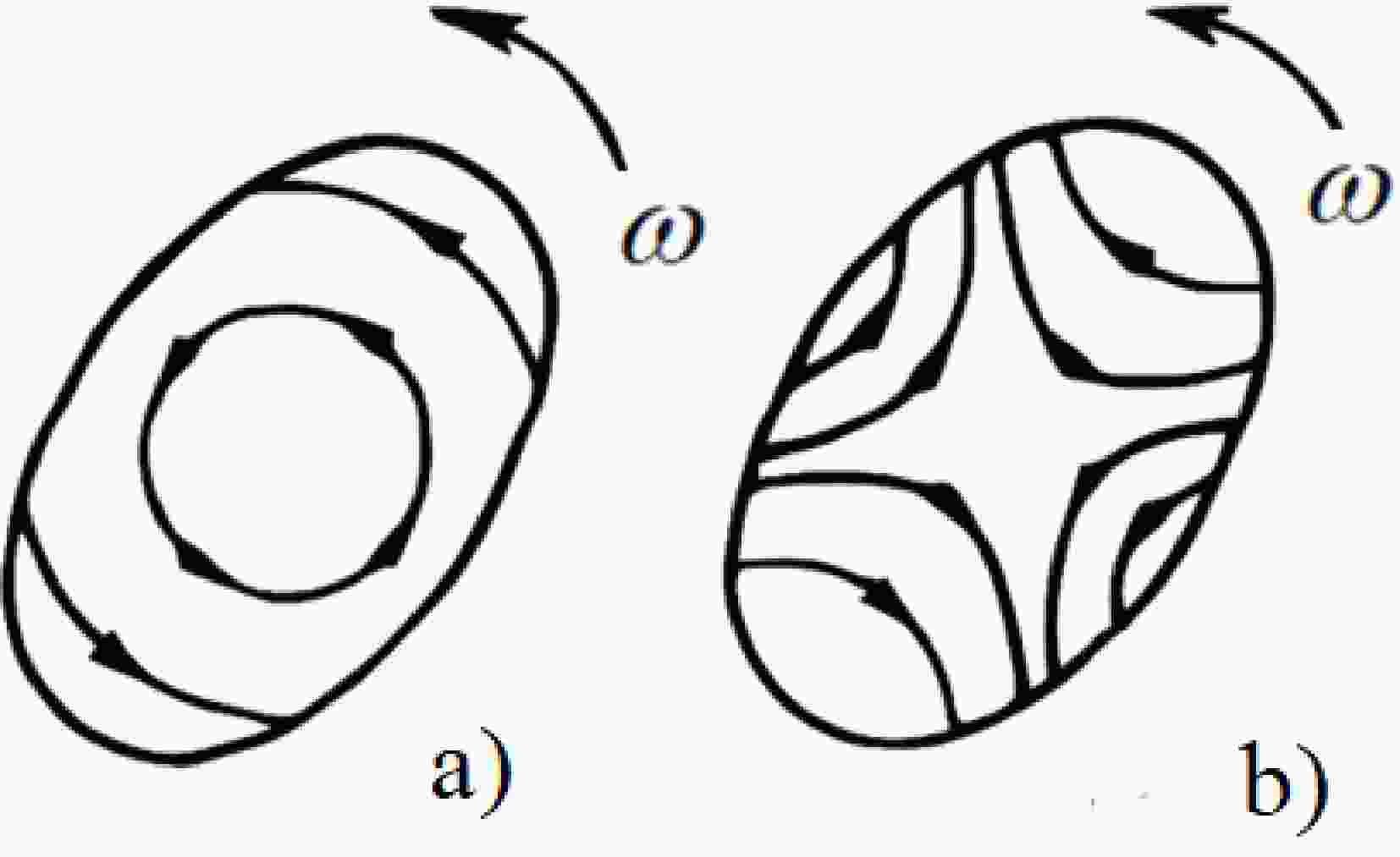
$\varphi $ that obeys the Laplace equation, that is,$ \Delta\varphi = 0 $ , and the velocity of the fluid v is determined by the potential gradient. For an ideal fluid, the boundary conditions simplify to the requirement that the normal component of the fluid velocity at the surface coincides with the normal component of the velocity at the vessel wall. In other words, while in the case of a solid body the entire system rotates as a whole, in the case of a rigid shell filled with an ideal fluid, the fluid is only entrained by the walls near the surface of the shell. A good illustration of the behavior of these velocity fields is shown in Fig. 1.
Figure 1. Velocity field in the case of rotation of a solid body (a) and potential motion of an ideal fluid in a rotating rigid shell (b).
When the nucleus is considered as a solid body, the moment of inertia has the form
$ \begin{aligned} J_0 = \frac{m}{5}\left(R_1^2 + R_2^2\right) = \frac{2}{5}mR^2 \left( 1 + \frac{1}{2}\sqrt{\frac{5}{4 {\text{π}}}}\beta + \frac{25}{32 {\text{π}}}\beta^2\right), \end{aligned} $

(3) where m is the mass of the nucleus. In the hydrodynamic model of the nucleus [12], the moment of inertia of the nucleus is represented as
$ \begin{aligned} J=\frac{m}{5}\frac{\left(R_2^2-R_1^2\right)^2}{R_2^2+R_1^2}, \end{aligned} $

(4) which, using Eq. (2), can be rewritten as
$ \begin{aligned} J=\dfrac{9mR^2}{4 {\text{π}}}\cdot \dfrac{\beta^2 \left(1+\dfrac{1}{4}\sqrt{\dfrac{5}{4 {\text{π}}}}\beta\right)^2}{2+\sqrt{\dfrac{5}{4 {\text{π}}}}\beta +\dfrac{25}{16 {\text{π}}}\beta^2}. \end{aligned} $

(5) When the deformation parameter β is small, both models have a relationship expressed as
$ \begin{aligned} \dfrac{J}{J_0}=\dfrac{45 \beta^2\left(1 + \dfrac{\beta}{4}\sqrt{\dfrac{5}{4 {\text{π}}}}\right)}{8 {\text{π}} \left(2 + \sqrt{\dfrac{5}{4 {\text{π}}}}\beta + \dfrac{25}{16 {\text{π}}}\beta^2 \right) \left(1 + \sqrt{\dfrac{5}{16 {\text{π}}}}\beta + \dfrac{25}{32 {\text{π}}}\beta^2 \right)}. \end{aligned} $

(6) Such a representation of the moment of inertia is convenient within the framework of the model of independent particles moving in a non-spherical well, for example in an anisotropically oscillating one, whose behavior is similar to the moment of inertia of a rigid body (Eq. (3)). This similarity arises because, during the slow adiabatic rotation of the potential well, the states of the individual, non-correlated particles do not change; as a result, the system behaves as a solid body during rotation.
Nevertheless, the observed moments of inertia of nuclei differ from the solid-state values, as demonstrated by extensive experimental data. These deviations are caused by residual interactions among nucleons, which slow down the collective rotation and reduce the moment of inertia of the system. If the interactions among particles were significant, their mean path length would be smaller than the size of the nucleus, resembling the behavior of the hydrodynamic model, where the collective motion of the nucleons becomes potential. In cases where the interactions among nucleons are dominated by pairing forces, a superfluid model of the nucleus must be applied. A consistent method for calculating the moments of inertia of nuclei based on this model was developed by Migdal [13], the main points of which are presented below.
-
Given that the atomic nucleus is a purely quantum system, the aforementioned solid-state and hydrodynamic approaches for estimating moments of inertia require corrections. The superfluid model of the nucleus and the many-particle shell model assume that the nucleons in the nucleus move as predicted by the single-particle shell model. Moreover, these models take into account the residual interactions, i.e., the correlations among the nucleons. In the superfluid model, residual interactions are treated using notably different and more sophisticated methods. Residual interactions are distinct from specific short-range pairing interactions, which play a crucial role in explaining the properties of nuclei. Experimental data (e.g., the binding energy of the last neutron in light nuclei and the zero spin of even-even nuclei in the ground state) suggest that strong correlations between two nucleons occur only when these nucleons occupy states with identical energy and quantum numbers, except for the projections of their total angular moments. In this context, the individual nucleons in the nucleus are assumed to have the same single-particle states as described in the independent-particle model. Thus, the pairing of nucleons can be effectively characterized using the quantum numbers of the aforementioned model.
The superfluidity of nuclei arises from the formation of nucleon pairs due to residual interactions among them. These pairs are a result of a specific type of correlation known as superconducting pair correlations. As a consequence, the ground-state energy of the nucleus is significantly lower than it would be in the absence of these correlations. This unique state of the nucleus is referred to as superfluid.
The effects of correlated pairs and superfluidity significantly influence the moments of inertia of nuclei. For example, owing to the superfluid properties of nuclei, the moments of inertia can be 2–3 times smaller than those predicted by analogous calculations using the solid state model. Consequently, the moments of inertia of nuclei were computed within the framework of superfluidity theory, which was originally developed for homogeneous, unbounded Fermi systems [14, 15].
Using Migdal’s approach [13], the moment of inertia for the oscillatory potential is expressed as
$ \begin{aligned} J=J_0\left\{1-g_1+\frac{g_1^2\chi^2}{v_1^2 g_1 + g^2_2\nu_2} \right\} = J_0 \Phi_1\left( \chi \right). \end{aligned} $

(7) Values of function
$ \Phi_1(\chi) $ are listed in Table 1 (for$ \nu_2 = 10 $ ). The parameter χ is defined by the expression$\chi $ 

$ \Phi_1 \left( \chi \right) $ 

$ \Phi_2 \left(\chi \right) $ 

$\chi $ 

$ \Phi_1 \left( \chi \right) $ 

$ \Phi_2 \left(\chi \right) $ 

$\chi $ 

$ \Phi_1 \left( \chi \right) $ 

$ \Phi_2 \left(\chi \right) $ 

0 0 0 0.9 0.43 0.17 1.8 0.77 0.34 0.1 0.01 0.01 1.0 0.49 0.19 1.9 0.79 0.36 0.2 0.03 0.02 1.1 0.53 0.21 2.0 0.80 0.37 0.3 0.07 0.03 1.2 0.60 0.23 2.2 0.81 0.40 0.4 0.13 0.06 1.3 0.64 0.24 2.4 0.83 0.43 0.5 0.19 0.08 1.4 0.67 0.26 2.6 0.85 0.45 0.6 0.26 0.10 1.5 0.71 0.28 2.8 0.86 0.48 0.7 0.32 0.13 1.6 0.74 0.30 3.0 0.87 0.50 0.8 0.38 0.15 1.7 0.75 0.32 Table 1. Values of functions
$ \Phi _1\left( \chi \right) $ and$ \Phi_2\left( \chi \right) $ defined within the superfluid model reported in [13].$ \begin{aligned} \chi =\frac{\varepsilon_0}{\Delta p_0 R_0} \cdot \beta, \end{aligned} $

(8) where
$ \beta =\dfrac{2\left( a - b \right)}{a + b} $ is the deformation parameter of the nucleus, a and b are the semi-axes of the spheroid;$ R_0=\dfrac{a+b}{2} $ ;$ p_0 $ is the momentum operator of the particle;$ \varepsilon_0 $ is the energy of the particle; and Δ is the mass defect.Within the framework reported in [13], it is possible to calculate the moment of inertia for a rectangular potential well introducing the variables
$ \eta = \dfrac{m}{l}{l} $ ,$ \xi = \dfrac{l}{l_0} $ :$ \begin{aligned}[b] J_1 & = J_0 \left\{ 1 - \frac{45}{4} \int\limits_0^1 {\rm d}\xi \xi^3\sqrt{1 - \xi ^2} \int\limits_0^1 {\rm d}\eta \left(1 - \eta^2 \right) g \left( \aleph \frac{\eta}{\xi} \right) \right\} \\ &= J_0 \Phi_2 (\chi). \end{aligned} $

(9) Values of function
$ \Phi_2 (\chi) $ are also listed in Table 1.The calculations in Table 1 were performed for only one type of nucleon. However, for the sake of comparison with experimental data, both types must be considered. When
$ Z > 20 $ , the Fermi levels of neutrons and protons diverge, making neutron-proton pairing impossible. From this point on, we assume that the nuclei consist of two fluids, neutron and proton, which cannot exchange the momentum of motion owing to the presence of an energy gap in the excitations of each fluid. In this case, the moment of inertia of the nucleus is represented as the sum of the moments of inertia of the neutrons and protons. Defining the ratio$ J_k / {J_0}_k = \Phi(\chi_k) $ , we obtain the expression$ \begin{aligned} \frac{J}{J_0}=\frac{N}{A}\Phi(\chi_n) + \frac{Z}{A}\Phi(\chi_p), \end{aligned} $

(10) where
$ \chi_n $ and$ \chi_p $ are values for neutrons and protons, respectively.The Δ values included in Eq. (8) cannot be calculated theoretically and must be experimentally measured. However, from the definition of the Green's function, we can obtain
$ \begin{aligned}[b] G_{\lambda}=&\sum\limits_s \frac{\left| \Phi _{N+1}^s, a_{\lambda}^+\Phi_N^0 \right|^2}{\varepsilon - E_s (N+1) + E_0 (N) + {\rm i}\delta} \\ &+\sum\limits_s \frac{\left| \Phi _{N-1}^s, a_{\lambda}\Phi _N^0 \right|^2}{\varepsilon +E_s (N-1) - E_0(N) - {\rm i}\delta}, \end{aligned} $

(11) where
$ a_{\lambda} $ and$ a_{\lambda}^+ $ are the particle annihilation and birth operators in the λ state.Comparing Eq. (11) with the expression provided in [13], it follows that
$ \begin{aligned} & E_0 (N+1) + E_0(N) = \Delta + \varepsilon_0, \\ & E_0 (N) - E_0 (N - 1)= -\Delta + \varepsilon_0. \end{aligned} $

(12) These formulas allow us to find Δ (MeV) from the binding energy of nuclei. A more accurate expression can be obtained by excluding
$ E_0(N) $ from the non-pairing dependence on N. For this purpose, we derive an expression in which the first and second derivative terms in the$ N' - N $ expansion are excluded. This condition is satisfied by$ \begin{aligned} \frac{1}{4}[3E (N+1) - 3E (N) + E (N-1) - E (N+2)] = \Delta. \end{aligned} $

(13) To compare Eqs. (7) and (8) with the moments of inertia experimentally measured, we express
$ \aleph $ and χ through the observed values. We obtain$ R_0 = R \left(1 + \dfrac{1}{3} \beta \right) $ . Given that$ R = 1.2 A^{1/3} \cdot 10^{-13} $ cm, we find that$ \begin{aligned}[b] &\varepsilon_{0}^n=52 \frac{M}{M_{\rm eff}} \left( \frac{N}{A} \right)^{2/3}\, , \\ &p_{0}^{n}R= 1.9 \cdot {N^{1/3}}\, , \\ &\chi_n=\frac{\beta}{1+\dfrac{\beta}{3}}\frac{27}{\Delta_n A^{1/3}}\left(\frac{N}{A} \right)^{1/3}. \end{aligned} $

(14) Similar expressions are obtained for protons:
$ \begin{aligned}[b] &\varepsilon_0^p = 52 \frac{M}{M_{\rm eff}} \left(\frac{Z}{A} \right)^{2/3} \;, \\ &p_0^p R=1.9\cdot Z^{1/3} \;, \\ &\chi_p=\frac{\beta}{1+\dfrac{\beta}{3}}\frac{27}{\Delta_p A^{1/3}}\left(\frac{Z}{A} \right)^{1/3}. \end{aligned} $

(15) The values of the moments of inertia of the nuclei were obtained using Eqs. (3), (5), (14), and (15). They were normalized to the solid moment of inertia. The results are presented in Fig. 2 and Table 2. Note that the best agreement between the experimental data and the different theoretical approaches is achieved within the framework of the oscillatory potential superfluid nucleus model. This was expected, because this approach takes into account the interactions among nucleons, which slow down the collective rotation, leading to a decrease in the moment of inertia of the system with respect to its solid-state counterpart. The observed overestimation of the moments of inertia of deformed fragments in equilibrium within a mass range from 150 to 200 is probably due to the use of oscillatory and rectangular well potentials, which constitutes a significant simplification. The use of more realistic or complex types of potentials would improve the description.
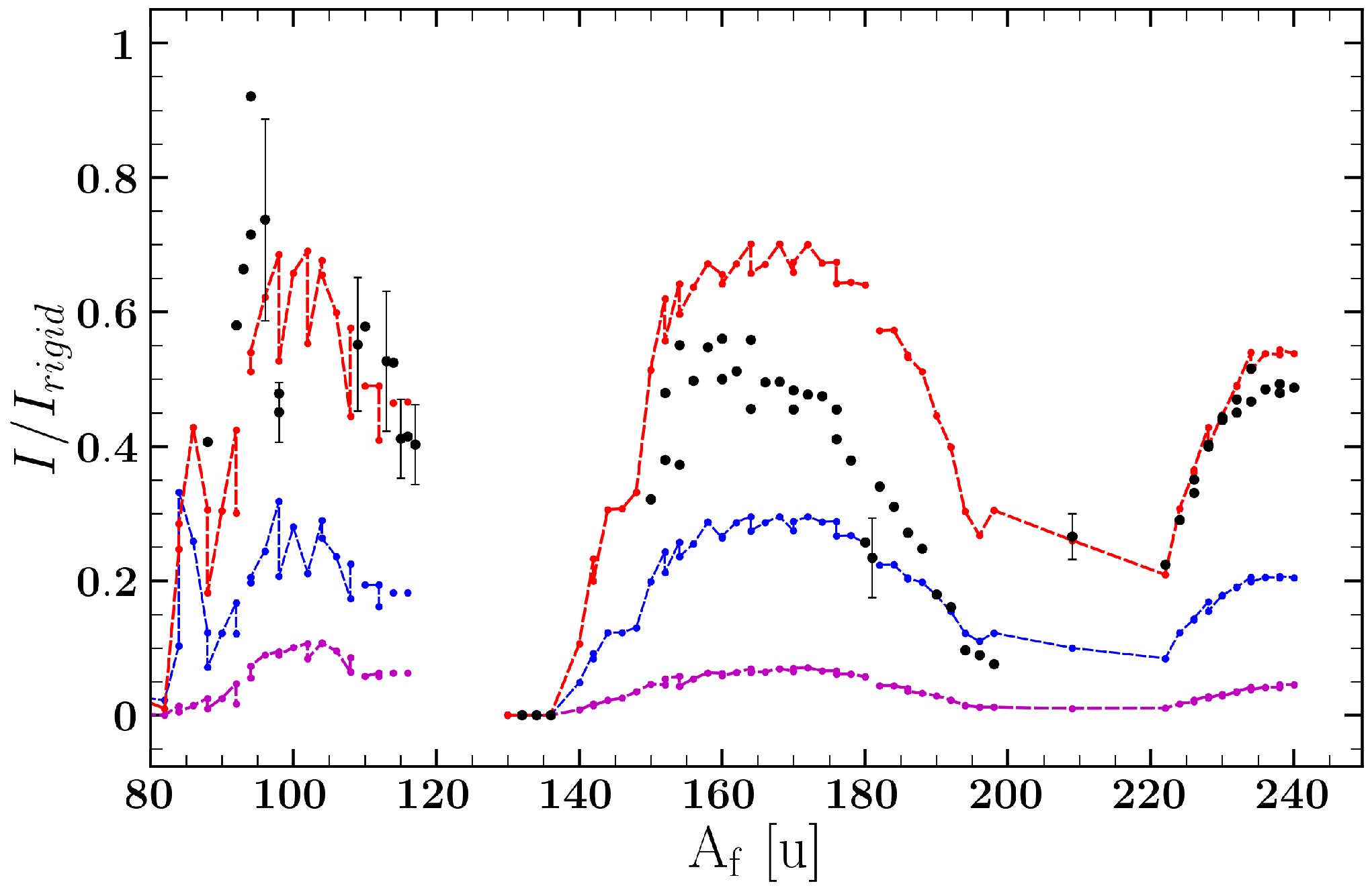
Figure 2. (color online) Comparison of the moments of inertia of nuclei as a function of their mass number
$ A_f $ calculated within the hydrodynamic approach (magenta) and the superfluid core model for the cases of rectangular (blue) and oscillatory (red). The black dots denote experimental data extracted from [16, 17]. All values are normalized to the values of the solid state moments.Nuclei $ {\Delta}_n $ 

$ {\Delta}_p $ 

$ {\chi}_n $ 

$ {\chi}_p $ 

β $J^{\rm osc}_{\rm sup}$ 

$J^{\rm rec}_{\rm sup}$ 

$J_{\rm hyd}$ 

$ {\rm ^{94}Sr} $ 

$ - $ 0.98

$ - $ 1.43

$ - $ 2.54

$ - $ 1.53

0.588 7.76 6.33 5.35 $ {\rm ^{158}Nd} $ 

$ - $ 0.64

$ - $ 0.91

$ - $ 4.64

$ - $ 2.76

0.892 12.10 10.50 9.10 $ {\rm ^{96}Sr} $ 

$ - $ 1.03

$ - $ 1.40

$ - $ 2.58

$ - $ 1.65

0.639 7.78 6.25 5.29 $ {\rm ^{156}Nd} $ 

$ - $ 0.67

$ - $ 0.89

$ - $ 4.35

$ - $ 2.80

0.867 11.82 10.08 8.66 $ {\rm ^{98}Sr} $ 

$ - $ 0.73

$ - $ 1.297

$ - $ 3.66

$ - $ 1.77

0.645 7.97 6.81 5.25 $ {\rm ^{154}Nd} $ 

$ - $ 0.69

$ - $ 0.62

$ - $ 4.21

$ - $ 4.03

0.864 11.87 10.88 8.53 $ {\rm ^{100}Zr} $ 

$ - $ 0.90

$ - $ 1.34

$ - $ 3.12

$ - $ 1.83

0.697 8.14 6.10 5.52 $ {\rm ^{152}Sm} $ 

$ - $ 1.12

$ - $ 1.12

$ - $ 2.49

$ - $ 2.12

0.813 11.28 8.34 8.28 $ {\rm ^{102}Zr} $ 

$ - $ 0.97

$ - $ 1.24

$ - $ 3.02

$ - $ 2.02

0.740 8.27 6.38 5.49 $ {\rm ^{150}Ce} $ 

$ - $ 0.79

$ - $ 1.03

$ - $ 3.35

$ - $ 2.20

0.759 11.25 8.84 7.59 $ {\rm ^{104}Zr} $ 

$ - $ 0.93

$ - $ 1.27

$ - $ 3.16

$ - $ 1.97

0.740 8.27 6.30 5.49 $ {\rm ^{148}Ce} $ 

$ - $ 1.00

$ - $ 1.27

$ - $ 2.65

$ - $ 1.80

0.759 10.77 8.07 7.39 $ {\rm ^{106}Mo} $ 

$ - $ 1.04

$ - $ 1.45

$ - $ 2.84

$ - $ 1.78

0.763 8.19 6.23 5.50 $ {\rm ^{146}Ba} $ 

$ - $ 0.95

$ - $ 1.23

$ - $ 2.68

$ - $ 1.67

0.715 10.54 7.89 6.76 $ {\rm ^{108}Mo} $ 

$ - $ 1.06

$ - $ 1.43

$ - $ 2.69

$ - $ 1.73

0.775 8.28 6.21 5.40 $ {\rm ^{144}Ba} $ 

$ - $ 0.92

$ - $ 1.19

$ - $ 2.63

$ - $ 1.74

0.668 10.10 7.36 7.47 $ {\rm ^{110}Ru} $ 

$ - $ 1.19

$ - $ 1.34

$ - $ 2.58

$ - $ 2.00

0.810 8.81 6.50 5.99 $ {\rm ^{142}Xe} $ 

$ - $ 0.94

$ - $ 1.13

$ - $ 2.42

$ - $ 1.41

0.615 10.20 7.41 5.70 $ {\rm ^{112}Ru} $ 

$ - $ 1.18

$ - $ 1.26

$ - $ 2.68

$ - $ 2.18

0.845 9.81 7.36 6.86 $ {\rm ^{140}Xe} $ 

$ - $ 0.98

$ - $ 1.22

$ - $ 2.30

$ - $ 1.58

0.604 10.79 7.51 5.93 $ {\rm ^{114}Pd} $ 

$ - $ 1.36

$ - $ 1.37

$ - $ 2.29

$ - $ 2.10

0.900 9.58 7.04 7.36 $ {\rm ^{138}Te} $ 

$ - $ 0.88

$ - $ 1.14

$ - $ 3.09

$ - $ 2.01

0.567 11.10 8.59 7.02 $ {\rm ^{116}Pd} $ 

$ - $ 1.30

$ - $ 1.35

$ - $ 2.47

$ - $ 2.18

0.938 9.74 7.06 7.70 $ {\rm ^{136}Te} $ 

$ - $ 0.83

$ - $ 1.12

$ - $ 2.57

$ - $ 1.62

0.559 10.56 7.70 5.04 $ {\rm ^{130}Sn} $ 

$ - $ 1.14

$ - $ 1.70

$ - $ 1.56

$ - $ 0.89

0.444 8.27 5.29 3.75 $ {\rm ^{122}Cd} $ 

$ - $ 1.30

$ - $ 1.34

$ - $ 2.67

$ - $ 2.25

0.997 10.58 8.01 8.07 $ {\rm ^{132}Sn} $ 

$ - $ 1.55

$ - $ 1.85

$ - $ 1.26

$ - $ 0.89

0.498 8.00 4.94 4.29 $ {\rm ^{120}Cd} $ 

$ - $ 1.32

$ - $ 1.32

$ - $ 2.60

$ - $ 2.27

0.976 10.32 7.69 8.08 $ {\rm ^{134}Te} $ 

$ - $ 1.48

$ - $ 0.94

$ - $ 1.42

$ - $ 1.93

0.549 9.45 6.19 4.91 $ {\rm ^{118}Pd} $ 

$ - $ 1.23

$ - $ 1.34

$ - $ 2.69

$ - $ 2.13

0.914 10.07 7.51 7.48 $ {\rm ^{136}Te} $ 

$ - $ 0.83

$ - $ 1.12

$ - $ 2.57

$ - $ 1.62

0.559 10.79 7.82 5.31 $ {\rm ^{116}Pd} $ 

$ - $ 1.30

$ - $ 1.35

$ - $ 2.60

$ - $ 2.18

0.938 10.56 7.88 7.88 $ {\rm ^{138}Xe} $ 

$ - $ 0.90

$ - $ 1.18

$ - $ 2.46

$ - $ 1.62

0.591 10.90 7.77 5.82 $ {\rm ^{114}Ru} $ 

$ - $ 1.17

$ - $ 1.20

$ - $ 2.75

$ - $ 2.30

0.865 10.24 7.72 7.23 $ {\rm ^{140}Xe} $ 

$ - $ 0.98

$ - $ 1.22

$ - $ 2.29

$ - $ 1.58

0.604 11.08 7.89 6.10 $ {\rm ^{112}Ru} $ 

$ - $ 1.18

$ - $ 1.27

$ - $ 2.68

$ - $ 2.15

0.845 10.07 7.51 7.00 $ {\rm ^{142}Xe} $ 

$ - $ 0.94

$ - $ 1.13

$ - $ 2.42

$ - $ 1.71

0.615 10.36 7.54 5.82 $ {\rm ^{110}Ru} $ 

$ - $ 1.19

$ - $ 1.34

$ - $ 2.63

$ - $ 2.01

0.817 9.09 6.71 6.15 $ {\rm ^{144}Ba} $ 

$ - $ 0.92

$ - $ 1.19

$ - $ 2.63

$ - $ 1.74

0.668 10.24 7.55 6.21 $ {\rm ^{108}Mo} $ 

$ - $ 1.06

$ - $ 1.44

$ - $ 2.83

$ - $ 1.79

0.775 8.40 6.26 5.58 $ {\rm ^{146}Ba} $ 

$ - $ 0.95

$ - $ 1.23

$ - $ 2.58

$ - $ 1.70

0.681 10.38 7.60 6.46 $ {\rm ^{106}Mo} $ 

$ - $ 1.04

$ - $ 1.47

$ - $ 2.85

$ - $ 1.74

0.763 8.32 6.23 5.49 $ {\rm ^{148}Ce} $ 

$ - $ 1.00

$ - $ 1.27

$ - $ 2.65

$ - $ 1.80

0.759 10.71 7.86 7.38 $ {\rm ^{104}Zr} $ 

$ - $ 0.93

$ - $ 1.27

$ - $ 3.15

$ - $ 1.97

0.740 8.24 6.21 5.48 $ {\rm ^{150}Ce} $ 

$ - $ 0.79

$ - $ 1.03

$ - $ 3.47

$ - $ 2.28

0.794 11.24 8.88 7.84 $ {\rm ^{102}Zr} $ 

$ - $ 0.97

$ - $ 1.24

$ - $ 3.00

$ - $ 2.02

0.729 8.21 6.38 5.48 $ {\rm ^{152}Nd} $ 

$ - $ 0.77

$ - $ 1.05

$ - $ 3.77

$ - $ 2.39

0.857 11.77 9.47 8.33 $ {\rm ^{100}Sr} $ 

$ - $ 0.78

$ - $ 0.79

$ - $ 3.54

$ - $ 2.97

0.673 8.18 6.68 5.81 $ {\rm ^{154}Nd} $ 

$ - $ 0.69

$ - $ 0.62

$ - $ 4.21

$ - $ 4.03

0.864 11.70 10.72 8.37 $ {\rm ^{98}Sr} $ 

$ - $ 0.73

$ - $ 1.30

$ - $ 3.66

$ - $ 1.76

0.645 7.69 6.53 5.05 Table 2. Values of
$ {\Delta }_n $ and$ {\Delta }_p $ calculated from mass defects for some elements.We explored several methods for estimating moments of inertia that yield more accurate theoretical predictions. These approaches also offer valuable insights into the dynamics of nuclear fission and the characteristics of the pre-fragment moments of inertia. However, a significant limitation is that these methods do not account for the substantial deformations of pre-fragments during fission. Additionally, no direct experimental technique currently exists to accurately determine their quadrupole nonequilibrium deformation parameters.
Nevertheless, the authors of the present study have devised an indirect method to estimate these deformations. Before introducing this method, it is essential to outline several key assumptions and concepts related to low-energy fission that will form the basis for the subsequent analysis.
-
To understand the main characteristics of the mentioned type of fission, quantum interference effects play a central role. These effects are described within the framework of quantum fission theory. In particular, the authors refer to findings from previous studies [18−26]. Within this framework, the nucleonic collective deformation and oscillation modes of the motion of the fissile nucleus are considered simultaneously, encompassing the evolution of its shape up to the point of scission into PFFs.
Thus, the characteristics of spontaneous nuclear fission can be described within the aforementioned framework using two fundamental assumptions proposed in a previous study [20]. First, throughout all stages of the fission process, the compound nucleus preserves its axial symmetry; this does not contradict existing experimental data. Second, during the descent from the outer saddle point to the scission point, the projection K of the spin J onto its symmetry axis Z is conserved, i.e., K remains an integral of motion. However, this conservation is not without challenges, given that the transient fissile state associated to K can be sensitive to thermal effects, both from the heating of the fissile nucleus prior to scission and from the heating of the PFFs in the early stages of their evolution. This is due to the fact that, for significant heating (
$ \approx 1 $ MeV) of an axial-symmetric nucleus, dynamical amplification of the Coriolis interaction occurs [24], leading to a uniform statistical mixing of all possible values of K projections at small values of spin J. In this case, all K projections near the scission point become equally probable, causing the complete disappearance of asymmetries [27, 28] , including different P and T parities, from the angular distributions of the products of binary and ternary fissions. Such anisotropies have been observed experimentally [29−36] even in the case of induced low-energy fission, where the excitation energies are higher than in spontaneous fission. It follows that within the framework of the considered type of fission, the composite nucleus remains "cold" at all stages, including the descent from the outer saddle point and formation of PFF angular distributions.For this reason, according to the "coldness" hypothesis of the fissile nucleus, we assume that all the excitation energy of the fission pre-fragments is "pumped" into collective deformation states, leading to their non-equilibrium deformation. After the breakup of the compound fissile system, the already heated FFs are de-excited according to a time constant
$ \tau_{\rm nuc} $ by neutron emission, from which the excitation energy of the FFs can be determined. For example, using the results reported by Strutinsky [37], which establish the relationship between the excitation energy and deformation of the fragments within the framework of the Liquid Drop Model (LDM), we can estimate the targeted value. In other words, the non-equilibrium pre-fragment deformations can be related to the average number of emitted neutrons from the specified FFs.The question that arises is related to the method for performing neutron yield estimation. In this study, two approaches were used.
The first approach involves the numerical calculation of the average number of emitted neutrons using the program package
$ \mathrm{FREYA} $ [3, 4, 38]. After the previously mentioned stages of PFF generation and nucleon exchange, the FF thermalization process is reproduced by successive neutron emissions. This process continues until the excitation energy of the FF falls below the threshold$ S_n + Q_{\rm min} $ , where$ S_n $ is the binding energy of the neutron in the FF and$ Q_{\rm min} = $ 0.01 MeV, i.e., the emission process occurs as long as it is energetically possible. When the neutron emission capability is exhausted, the excited FFs release the remaining excitation by emitting gamma quanta.The second approach, developed in [39], is based on the theoretical evaluation of FF decay considering the conservation laws of total angular momentum and parity. This approach is time-consuming, given that it requires the collection of substantial initial data, particularly on excitation characteristics such as level density and discrete level diagrams. The challenge is further aggravated by the fact that FFs are neutron-excess nuclei, making experimental data on neutron resonance density difficult to obtain. A solution was implemented by using a data library developed under the auspices of the IAEA by an international group of experts. This library facilitates theoretical calculations of nuclear reaction cross sections. [40]. However, this solution only included nuclei for which neutron resonance densities were known. The data for discrete levels, sourced from the NUDAT database (version of February 23, 1996), contained several fundamental and technical errors. To address this, Grudzevich developed a new library, LDPL-98, which incorporates density parameters and discrete level diagrams, as well as data for over 2,000 nuclei far from the stability line. This library allows for more accurate estimations of spectra and cross sections for these nuclei. Another distinction of this approach is that neutron yields were calculated exclusively for those FFs where the ratio of the experimental value for a given fragment to the maximum neutron yield was at least
$ 0.1 $ . In [38], all nuclei for which neutron multiplicity data were available were considered.Figure 3 presents calculations based on the approaches described above, alongside available experimental data extracted from [41]. Within the framework of the theoretical models, multiplicities have been calculated for FFs with mass numbers ranging from 80 to 160. Note that the calculations performed in
$ \mathrm{FREYA} $ are qualitatively similar to the experimental data. However, the approach described in [39] exhibits better agreement with the experimental values.
Figure 3. (color online) Mean neutron multiplicities as a function of the mass of spontaneous fission fragments
$ \rm^{252}Cf $ . The black dots represent experimental data extracted from [41], the red line represents estimations from the$ \mathrm{FREYA} $ model, and the blue line represents the evaluation method proposed by Grudzevich [39].Next, we determine the excitation energy U. Using the formula proposed in [39] that relates the excitation energy U and neutron multiplicity, we obtain
$ \begin{aligned} U=5+4\nu +{\nu }^2, \end{aligned} $

(16) where ν is the neutron multiplicity. The nonlinearity of the function may indicate that the average energy carried away by neutrons increases with their number as the remaining nucleus approaches the stability line.
Applying Eq. (16), we obtained the averaged excitation energies
$ \overline{U} $ shown in Fig. 4, where the red line represents results obtained from FREYA, the blue line corresponds to data calculated in [39], and the black dots represent energies derived from experimental data [41]. From a comparative analysis of Fig. 4, it can be concluded that there is a reasonable agreement of the considered approaches in terms of preservation of the sawtooth structure for neutron yield multiplicity and excitation energy.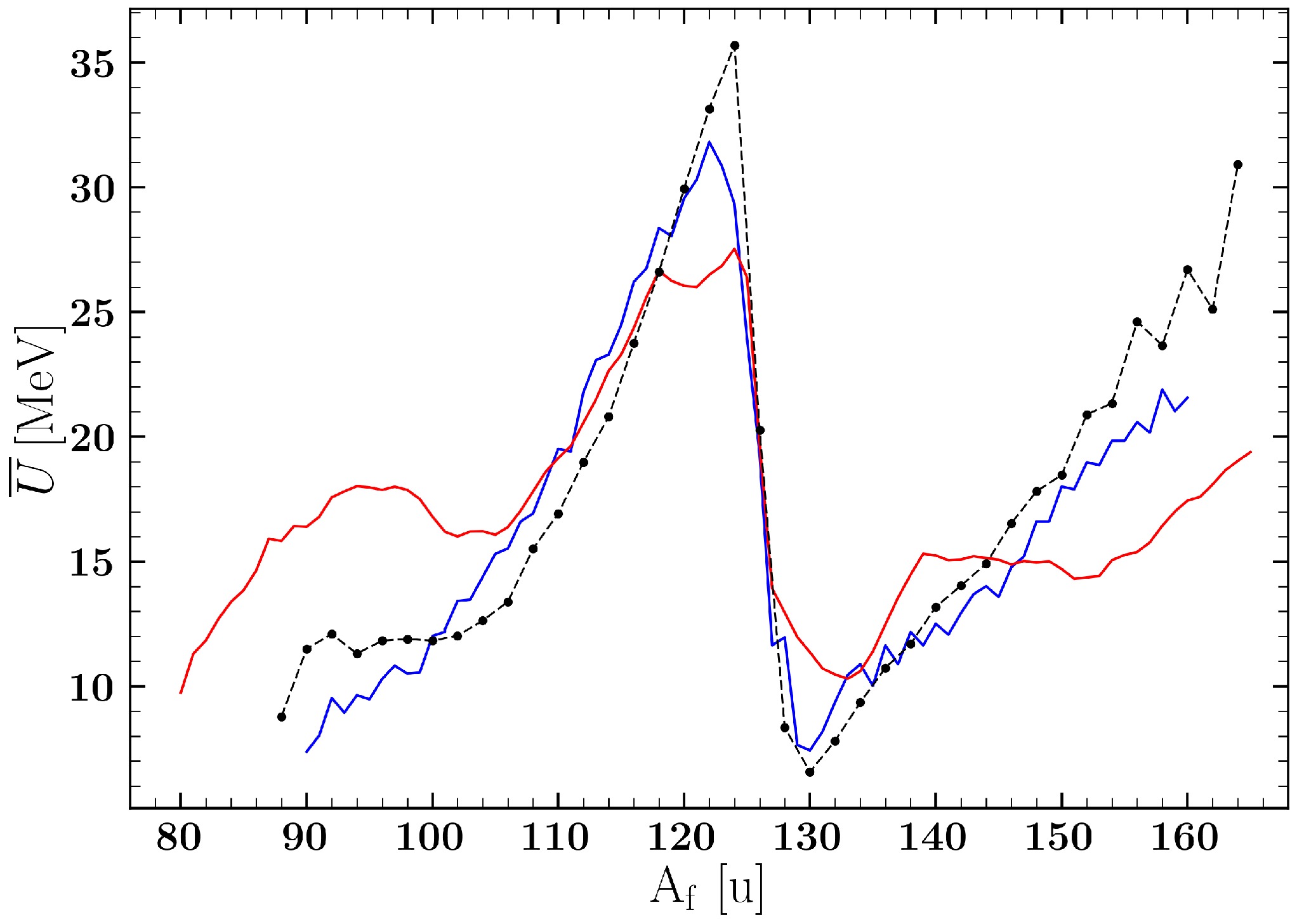
Figure 4. (color online) Mean excitation energies as a function of spontaneous fission fragment mass
$ \rm^{252}Cf $ . The black dots along with the dashed line represent reconstructed excitation energies from the data in [41], the red line represents results from$ \mathrm{FREYA} $ , and the blue line represents estimations obtained by the method proposed by Grudzevich [39].The final step is to establish the relationship between the excitation energy of the FF and its non-equilibrium deformation. For this purpose, we used the method proposed in [37], as already mentioned. Strutinsky suggested using the Nilsson level scheme to calculate the shell correction to the energy obtained using the LDM as a function of the occupation number and deformation. This author found a strong correlation between the shell correction and the density of nucleon levels at the Fermi energy. In this case, we suppose that the excitation energy U is represented as the deformation energy calculated within the LDM framework, which is the sum of the surface and Coulomb energies expressed in a simple form as
$ \begin{aligned} U=\sigma A^{2/3}\left[ 0.4 ( 1 - x )\alpha^2 - 0.0381( 1 - 2 x ) \alpha^3 \right], \end{aligned} $

(17) where the coefficients are
$ \sigma =16 $ MeV,$ x= Z^2 / \left( 45 \cdot A \right) $ , and α is related to the deformation parameter by the ratio$ \alpha =\dfrac{2}{3}\beta $ .Eq. (17) can be employed to calculate the equilibrium deformation energy by inserting the equilibrium deformation values extracted from [42]. Given that neither the results from
$ \mathrm{FREYA} $ nor the results reported by Grudzevich are in full agreement with the experimental data [41], it seems most reasonable to obtain the excitation energies using Eq. (16). By adding the excitation energy calculated from the evaluation to the equilibrium values of the deformation energy, we obtained the non-equilibrium excitation energy. Then, using the given data and Eq. (17), the inverse problem is solved, and hence, the non-equilibrium deformations of the fission pre-fragments are determined. All these values are listed in Table 2. -
With this information, it is finally possible to identify the most correct model for the moments of inertia. Given that there is currently no experimental method capable of estimating the moments of inertia of deformed FFs, we proceed indirectly. The proposed method consists in comparing the mean values of the FF spins with their analogous experimental values extracted from [43] for the case of spontaneous fission
$ \rm ^{252}Cf $ . For this purpose, we use the apparatus proposed in [44]. Given that the fragments emitted from the fissile nucleus in the vicinity of the scission point must be at "cold" non-equilibrium states [26], one should consider only zero oscillatory wave functions in the momentum representation [28, 44] when constructing their mean values:$ \begin{aligned}[b] P \left(J_{k_x},J_{k_y} \right) &= P (J_{k_x}) P(J_{k_y}) \\ & = \frac{1}{ {\text{π}} I_k \hbar \omega _k} \exp \left[ - \frac{J_{k_x}^2 + J_{k_y}^2}{I_k \hbar \omega_k}\right], \end{aligned} $

(18) where k denotes the type of bending (b) or wriggling (w) oscillations, and the energies of the indicated zero oscillations [19] are
$ \hbar {\omega }_w=2.5 $ MeV and$ \hbar {\omega }_w=0.9 $ MeV, respectively. Using this form of spin distributions and performing a number of simple transformations, one can derive the following expression to calculate the mean value of the PFF spins:$ \begin{aligned} \overline{J_i}=\int\limits_{0}^{\infty }{{J_1}\frac{2{J_1}}{d_i}\exp \left[ \frac{J_{1}^{2}}{d_i} \right]{\rm d}{J_1}}=\frac{\sqrt{ {\text{π}} {d_i}}}{2}, \end{aligned} $

(19) where
$ d_i = \dfrac{I_i^2}{(I_1 + I_2)^2} I_w \hbar \omega_w + I_b \hbar \omega_b $ , with$i= 1,2$ being the fragment index.Eq. (19) can be employed to obtain estimates using three distinct models of moments of inertia. The results are presented in Fig. 5.
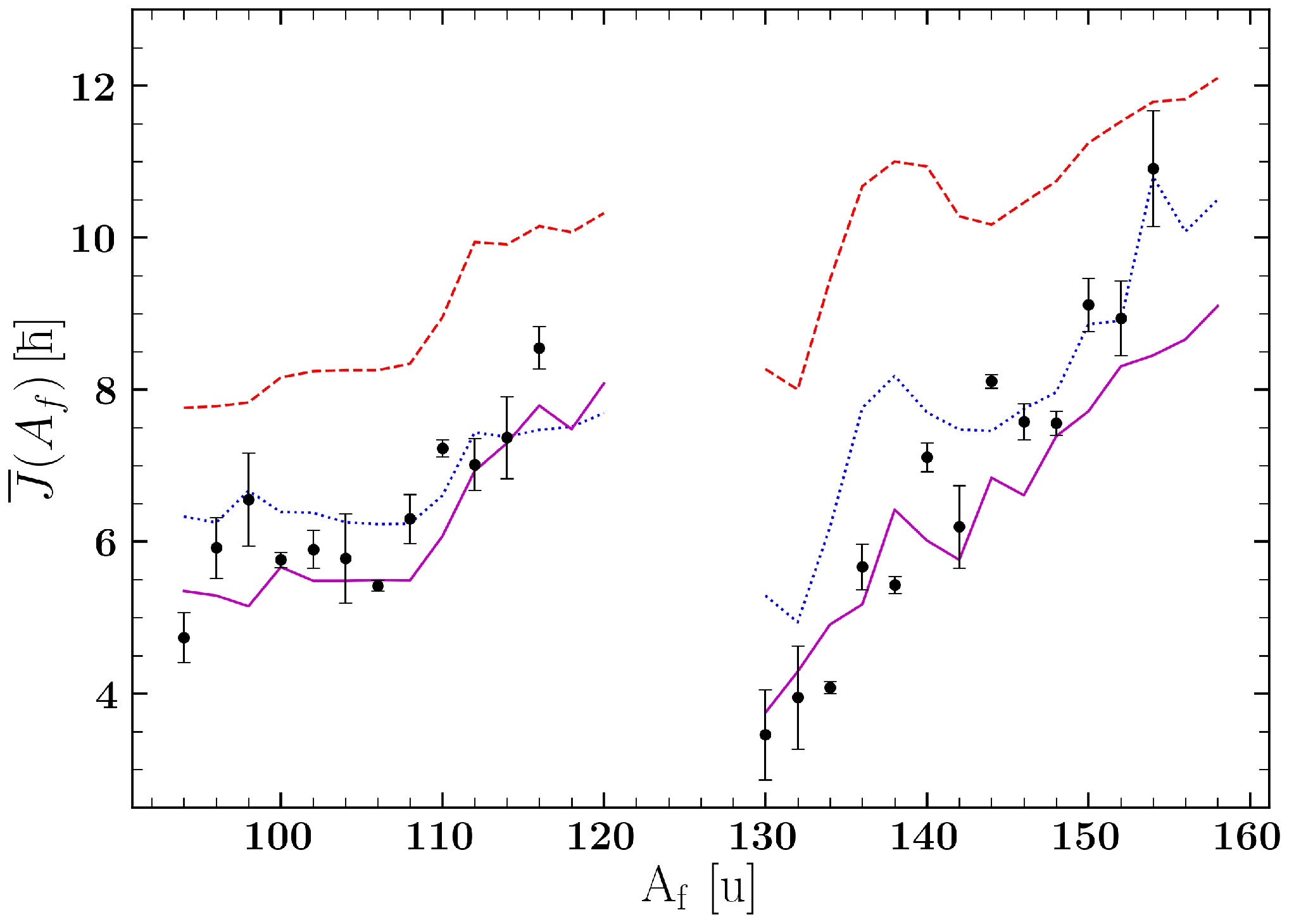
Figure 5. (color online) Mean spin of FFs as a function of their mass for the spontaneous fission
$ \rm ^{252}Cf $ , obtained using three estimates of the moments of inertia. For the superfluid approach, the mean spin is represented by the red dashed line in the case of an oscillatory potential; the blue dashed line represents the case of a rectangular potential for the hydrodynamic model. The magenta line represents experimental points extracted from [43].Comparing the obtained theoretical curves with the experimental data reported in [43], a qualitative agreement can be observed only for the magenta line, i.e., for estimates of the moments of inertia within the hydrodynamic model. By contrast, the mean spin values calculated following the superfluid approach in rectangular and oscillatory potentials (blue and red dashed lines) are in poor agreement, especially for the latter.
This apparently contradictory picture is extremely interesting, because it shows that, as long as the FFs have small quadrupole deformations slightly deviating from spherical symmetry, the Cooper pairing and superfluid nucleon-nucleon correlations work well. Therefore, the best results were obtained using a superfluid model with an oscillatory potential, as shown in Fig. 2. However, as soon as PFFs move into non-equilibrium deformations, where they reach abnormally large values (close to 1), the mean path length becomes smaller than the nucleon size. Thus, the hydrodynamic model begins to prevail and the collective motion of the nucleons becomes potential, as can be seen from the analysis shown in Fig. 5 and Table 2.
The analysis of pre-fragment moments of inertia at the rupture point has revealed that accurately describing these moments requires accounting for various factors, including changes in fragment states at different stages of fission. This underscores the complexity of the behavior of PFFs and highlights the limitations of relying on a single model to describe these processes. Furthermore, it emphasizes the need for a unified quantum fission theory capable of encompassing both the formation of PFF moments of inertia and their associated spins, thereby raising a more fundamental question about the mechanisms underlying nuclear fission.
Given that it is crucial to use the most complete and reliable experimental dataset, the spontaneously fissile nucleus
$ ^{252} $ Cf was chosen as the nucleus to study. In the following section, a detailed physical justification of why this isotope was chosen is provided. Moreover, we discuss the limitations associated with the availability of data for the other nuclei. -
Initially, this study was intended to be broader, encompassing additional actinide nuclei capable of undergoing spontaneous fission, such as
$ ^{238} $ U,$ ^{238-242} $ Pu,$ ^{244,248} $ Cm, and$ ^{252} $ Cf, in order to conduct a more comprehensive comparative analysis. However, we encountered the problem of limited experimental data.Note that, according to the methodology proposed in Sec. III, experimental data on multiplicities of instantaneous neutrons are required to perform the calculations. This immediately reduced the selection to three isotopes, namely
$ ^{244,248} $ Cm and$ ^{252} $ Cf, because the mentioned values were only found for them in the EXFOR [45] database; they are described in [41, 46]. Moreover, the comparison of the spin distributions calculated using our model requires the availability of analogous experimental distributions, which proved to be a challenging task.In addition to the previously discussed results for
$ ^{252} $ Cf, detailed in [43], analogous experimental data for heavy FFs were reported in [47]. However, the veracity of these data is questionable, mainly because the size of the spins was overestimated in that study. This discrepancy is evident in Fig. 6, which provides a visual representation of the comparison. Interestingly, there is a double excess of spin values within the mass interval of$ 128 \le A_f \le 142 $ , which indicates that this region is close to magic nuclei. As can be seen in Fig. 1, a clear contradiction arises: the fragments in this region are expected to have small moments of inertia, which determine the spin formation, as correctly noted in [2]. However, as$ A_f $ increases, the spin values begin to align with the experimental data presented in [43], in accordance with the prevailing theoretical understanding. The observed discrepancy underscores the necessity for employing only updated data for a valid comparison.
Figure 6. (color online) Comparison of the experimental values of mean spins as a function of the FF masses of spontaneous fission fragments of
$ ^{252} $ Cf. The results in red represent the findings of previous studies referenced in [47], while the results in blue represent the findings of more recent studies [43].With regard to the curium isotopes, we were unable to identify any recent distributions for these isotopes, despite their inclusion in previous studies [48, 49]. First, spin data for
$ ^{248} $ Cm were considered, wherein data are available for both light and heavy FFs [48]. The spin distributions for three models of FF moments of inertia were constructed using the method described above and subsequently compared with the experimental values presented in Fig. 7. As illustrated in this figure, there is a notable divergence between the hydrodynamical approach and the superfluid model with oscillatory potential in the near-magic region, that is,$ 136 \le A_f \le 142 $ . Only the rectangular potential model exhibits qualitative agreement, but this is limited to a specific region. All approaches maintain the sawtooth character, which is consistent with the results for the spontaneous fission of$ ^{252} $ Cf.
Figure 7. (color online) Mean spin values from the FF mass number of the spontaneous fission of the
$ ^{248} $ Cm nucleus. The red dashed line corresponds to the superfluid approach with an oscillatory potential; the blue dotted line represents the rectangular potential; the magenta line corresponds to the hydrodynamic approach. The black circles represent experimental points extracted from [46, 48].These results reveal a probable overestimation of the values in the previously used data. To illustrate this point, we compare the distributions in Fig. 8. As can be observed in the lower panel, the distributions for
$ ^{248} $ Cm, as reported in [48], are generally consistent with the behavior of$ ^{252} $ Cf, as reported in [43]. However, as these distributions approach the magic nuclei, a significant discrepancy emerges, similar to the overestimated data presented in [47]. It is important to note the discrepancy of more than$ \hbar $ in favor of$ ^{248} $ Cm, which is questionable. It seems unlikely that the addition of a few neutrons and protons would have a significant impact on the spin distribution. Accordingly, an examination of the experimental data for$ ^{244} $ Cm as presented in the upper panel of the referenced figure is not necessary, given that its behavior does not significantly differ from the previously discussed cases of$ ^{252} $ Cf.
Given that the data from [47−49] could not be corroborated by modern experiments [43], only the empirical outcomes have been employed to evaluate the models. The absence of contemporary and reliable data for other isotopes, including both
$ ^{244} $ Cm and$ ^{248} $ Cm, has thus limited our study of spontaneous fission of$ ^{252} $ Cf, for which experimental data are most reliable. -
In this study, a comprehensive and detailed examination of various theoretical models proposed for describing FF moments of inertia was conducted. Data analysis yielded several key conclusions.
The "direct" approach, described in Subsection II.B, based on a superfluid model of the nucleus with an oscillatory potential, shows the closest agreement with experimental results. This model is particularly effective when considering small quadrupole deformations near spherical symmetry, where residual interactions, such as Cooper pairing and superfluid nucleon-nucleon correlations, play a significant role. Under these conditions, the mean path length of nucleons is approximately equal to the size of the nucleus, thereby further validating the applicability of the model.
In contrast, the "indirect" approach, discussed in Subsection III.B, which compares models based on the average values of spins, was found to be less reliable. Agreement is only achieved when a hydrodynamic model is used, which becomes dominant under conditions of substantial quadrupole deformation. In this scenario, the mean path length of nucleons is smaller than the size of the nucleus, allowing the hydrodynamic model to more accurately capture the dynamics of fission.
These findings underscore the importance of employing diverse models in accordance with the prevailing nuclear deformation conditions. This distinction is pivotal not only for advancing theoretical understanding but also for practical applications, e.g., the development of computational tools such as
$ \mathrm{FREYA} $ . For instance, the authors of$ \mathrm{FREYA} $ used the "ad hoc" approximation for moments of inertia, which is less accurate than the approaches discussed in this study.The results presented in this article are unique in that they provide the first comparative analysis of FF moments of inertia using two distinct approaches. This study establishes a basis for further research that should extend these findings across a broader range of nuclei, thereby facilitating a more precise determination of the applicability of each model. Such endeavors will advance the frontiers of current quantum fission theory.
In terms of extending the scope, the analysis revealed significant discrepancies between the FF spin distributions obtained more than a few decades ago and modern data. The older data for the nuclei in question, namely
$ ^{244} $ Cm,$ ^{248} $ Cm, and$ ^{252} $ Cf, exhibit spin values exceeding the actual values, raising concerns about the precision of the data. The high spin values for the FF of the actinide nuclei in the near-magic region are in significant disagreement with modern concepts, whereas recent data for$ ^{252} $ Cf are in good agreement with current theoretical models. This highlights the necessity for further experimentation with other isotopes to resolve existing uncertainties and enhance the precision of theoretical models.This study emphasizes the critical importance of understanding the nature of FF moments of inertia and their role in nuclear fission, providing valuable insights to the field and creating opportunities for future research.
-
Authors are very grateful to Prof. S.G. Kadmensky for help and discussions on clarifying details on the "coldness" of the fissile nucleus. They are also very grateful to Prof. V.I. Furman for useful comments and interesting discussions on the present study.
Evaluation of fission fragment moments of inertia forspontaneous fission of CF-252
- Received Date: 2024-08-27
- Available Online: 2025-03-15
Abstract: In the present study, methods for estimating the moments of inertia of fission fragments resulting from the spontaneous fission of isotope Cf-252 were analyzed. In particular, two main approaches were examined: statistical and microscopic. The classical and superfluid approaches for calculating the moments of inertia were also examined, along with their implementations in a variety of nuclear models. In this context, the impact of diverse oscillation modes and nucleon exchange on the moments of inertia and spin distributions of fission fragments was assessed. This study emphasizes the need for a comparative analysis of theoretical predictions and experimental data, which would contribute to a more comprehensive understanding of the internal structure of nuclei and the mechanisms of fission.


 DownLoad: