SU(3) analysis for B(E2) anomaly

Understanding the deformations of nuclei and their changes, continuous or abrupt, is one of the fundamental problems in the field of nuclear structure. Quadrupole deformations are the most important. The geometrical model with deformation variables β and γ has given a good description, where β represents the degree of deviation from the spherical shape and γ presents the angle for describing the triaxial deformation. 50 years ago, the interacting boson model (IBM) was proposed [1, 2], which is an algebraic model for describing the collective excitations (deformations) in nuclear structure. For the simplest case, only the s and d bosons with angular momentum $ L = 0 $ and $ L = 2 $ respectively are considered to construct the Hamiltonian, which has the U(6) symmetry. Four dynamical symmetry limits exist: the U(5) symmetry limit (spherical shape), the SU(3) symmetry limit (prolate shape), the O(6) symmetry limit (γ-soft rotation) and the $ \overline{ {\rm{SU(3)}}} $ symmetry limit (oblate shape) [3]. Shape phase transitions between different shapes can be also studied by this model [4−18]. Thus, the IBM provides an efficient theoretical framework to describe various deformations of nuclei and their collective excitation behaviors, thus it has a broad impact in the field of nuclear structure.

Although previous IBM is self-consistent for describing various quadrupole deformations, some of the experimental anomalies seem to be indescribable by previous model hamiltonians, such as the B(E2) anomaly [19−22] and the Cd puzzle [23−28]. In the B(E2) anomaly, the ratio $ E_{4/2} = E_{4_{1}^{+}}/E_{2_{1}^{+}} $ of the energies of the $ 4_{1}^{+} $, $ 2_{1}^{+} $ states is larger than 2.0 (a feature for the collective excitations), but the ratio $ B_{4/2} = B(E2;4_{1}^{+}\rightarrow 2_{1}^{+})/B(E2;2_{1}^{+}\rightarrow 0_{1}^{+}) $ of the E2 transitions $ B(E2;4_{1}^{+}\rightarrow 2_{1}^{+}) $ and $ B(E2;2_{1}^{+}\rightarrow 0_{1}^{+}) $ can be much smaller than 1.0 (a traditional signal for the non-collective behaviors), which cannot possibly be explained by previous theories in nuclear structure [19−22]. In the Cd puzzle, the experimental data did not confirm the phonon excitations of the spherical nucleus [23−27], and questioned its existence [28]. Experimentally, the B(E2) anomaly and the Cd puzzle can occur in adjacent nuclei, such as $ ^{72-76} {\rm{Zn}}$ [29−31] and even in a single nucleus, such as $ ^{114} {\rm{Te}}$ [32, 33], so they may have a common origin.

Moreover, it was found that nuclei previously considered as prolate shape should be rigid triaxial [34−36], making previous IBM descriptions not particularly convenient. In previous IBM, the spectra of the prolate shape (the SU(3) symmetry limit) and the oblate shape (the $ \overline{ {\rm{SU(3)}}} $ symmetry limit) are the same [3], but this mirror symmetry can not be found in realistic nuclei [37].

Therefore, it is necessary to make further generalization based on the existing models. Recently an extension of the interacting boson model with SU(3) higher-order interactions (SU3-IBM) was proposed to resolve these various anomalies. In the SU3-IBM, by introducing the SU(3) third-order and fourth-order interactions, the SU(3) symmetry limit can describe not only prolate shape (SU(3) second Casimir operator $ -\hat{C}_{2}[ {\rm{SU(3)}}] $), but also oblate shape ($ \hat{C}_{3}[ {\rm{SU(3)}}] $) and various rigid triaxial shapes (combinations of $ -\hat{C}_{2}[ {\rm{SU(3)}}] $, $ \hat{C}_{3}[ {\rm{SU(3)}}] $ and $ \hat{C}_{2}^{2}[ {\rm{SU(3)}}] $), and even dynamical effects independent of the ground state. Thus the SU(3) symmetry plays a more important role.

Through detailed discussions, it was found that this model can better describe the collective behaviors of atomic nuclei. It can describe the B(E2) anomaly and the Cd puzzle [38, 39]. Although the B(E2) anomaly can not be described by previous nuclear theories [19−22], many possible explanations exist in the SU3-IBM and other extended IBM theories [40−48]. The spherical-like spectra for resolving the Cd puzzle were really found in $ ^{106} {\rm{Pd}}$ [49]. The SU3-IBM can be also used to explain the prolate-oblate shape asymmetric transitions in the Hf-Hg region [50−52], to describe the γ-soft behaviors in $ ^{196} {\rm{Pt}}$ at a better level [53], to describe the E(5)-like spectra in $ ^{82} {\rm{Kr}}$ [54], and to explain the unique boson number odd-even phenomenon in $ ^{196-204} {\rm{Hg}}$ [55] which was first found in [51]. Furthermore it can well describe the rigid triaxiality in $ ^{166} {\rm{Er}}$ [56]. Recently the shape phase transition from the new γ-soft phase to the prolate shape is also found and $ ^{108} {\rm{Pd}}$ is the critical nucleus [57]. These results have overturned our traditional understanding of nuclear structure, because it has captured almost all the shape patterns and given new collective patterns for describing various anomalous behaviors.

Based on previous results [40−48], we continue to discuss the mechanisms in the B(E2) anomaly. So far, many possible explanations have been found for the B(E2) anomaly. Some more fundamental discussions can make some key parts clearer. We introduce the concept “SU(3) analysis”, which is used to reanalyse the results obtained in these studies within the SU(3) symmetry limit. Remove the non-SU(3) symmetry parts of the Hamiltonian to discuss whether the remaining SU(3) symmetry part can have the B(E2) anomaly ($ B(E2;4_{1}^{+}\rightarrow 2_{1}^{+}) = 0 $). If it happens, it may be the reason for the emergence of the B(E2) anomaly in the original Hamiltonian. For the remaining SU(3) symmetry part, when the parameter in front of the SU(3) third-order interaction $ [L\times Q \times L]^{(0)} $ changes, the partial low-lying levels and the values of $ B(E2;2_{1}^{+}\rightarrow 0_{1}^{+}) $, $ B(E2;4_{1}^{+}\rightarrow 2_{1}^{+}) $ and $ B(E2;6_{1}^{+}\rightarrow 4_{1}^{+}) $ are discussed. We find three new results: (1) The interaction $ [L\times Q \times L]^{(0)} $ is critical for the SU(3) anomaly; (2) Level-crossing within the SU(3) symmetry limit is crucial for the SU(3) anomaly; (3) Not only the value of $ B(E2;4_{1}^{+}\rightarrow 2_{1}^{+}) $ but also the ones of $ B(E2;6_{1}^{+}\rightarrow 4_{1}^{+}) $ and $ B(E2;2_{1}^{+}\rightarrow 0_{1}^{+}) $ can be anomalous (these values can be 0). Thus the SU(3) analysis is a useful tool for identifying the real cause. We expect it can be used in future discussions on the B(E2) anomaly.

In the SU3-IBM, the U(5) symmetry limit and the SU(3) symmetry limit are included (some bias towards the O(6) symmetry may be also required). In the SU(3) symmetry limit, the SU(3) second-order Casimir operator $ -\hat{C}_{2}[ {\rm{SU(3)}}] $ can describe the prolate shape and the SU(3) third-order Casimir operator $ \hat{C}_{3}[ {\rm{SU(3)}}] $ can describe the oblate shape, which fundamentally distincts from previous IBM [52]. The rigid triaxial shape can be obtained by the combinations of the square of the SU(3) second-order Casimir operator $ \hat{C}_{2}^{2}[ {\rm{SU(3)}}] $ and the $ -\hat{C}_{2}[ {\rm{SU(3)}}] $, $ \hat{C}_{3}[ {\rm{SU(3)}}] $. Moreover, the SU(3) invariants $ [L\times Q \times L]^{(0)} $ and $ [(L \times Q)^{(1)}\times (L \times Q)^{(1)}]^{(0)} $ are necessary.

The Hamiltonian is as follows

where α, β, γ, δ, η, ζ and ξ are seven fitting parameters. $ \hat{n}_{d} = d^{\dagger}\cdot \tilde{d} $ is the d boson number operator. $ \hat{Q} = [d^{\dagger}\times\tilde{s}+s^{\dagger}\times \tilde{d}]^{(2)}-\frac{\sqrt{7}}{2}[d^{\dagger}\times \tilde{d}]^{(2)} $ is the SU(3) quadrupole operator and $ \hat{L} = \sqrt{10}[d^{\dagger}\times \tilde{d}]^{(1)} $ is the angular momentum operator. The first four interactions determine the quadrupole shapes of the ground state of the nucleus, and the positions of the $ 0^{+} $ states of the excited levels. The latter three ones are the dynamical interactions and can be used to change the features of the non-$ 0^{+} $ states.

The two SU(3) Casimir operators have relationships with the quadrupole second or third-order interactions as follows:

For a given SU(3) irreducible representation $ (\lambda,\mu) $,the eigenvalues of the two Casimir operators under the group chain $ {\rm{U(6)}} \supset {\rm{SU(3)}} \supset {\rm{O(3)}} $ are expressed as

The SU(3) irreducible representation $ (\lambda,\mu) $ can have relationships with the quadrupole deformation variables β and γ as follows

and

where $ \beta_{0} $ is a scale factor.

For understanding the B(E2) anomaly, the B(E2) values are necessary. The $ E2 $ operator is defined as

where q is the boson effective charge. The evolutions of $ B(E2; 2_{1}^{+}\rightarrow 0_{1}^{+}) $, $ B(E2; 4_{1}^{+}\rightarrow 2_{1}^{+}) $, $ B(E2; 6_{1}^{+}\rightarrow 4_{1}^{+}) $ values are discussed.

Although the B(E2) anomaly can not be explained by previous nuclear structure theories, in the extended IBM with higher-order interactions, it can be described by many ways [40−48]. A key problem is that whether these explanations are related to the SU(3) symmetry. Obviously, this needs to consider these explanations in the SU(3) symmetry limit. For explaining the B(E2) anomaly in the realistic nuclei, the boson number operator $ \hat{n}_{d} $ is needed in some descriptions or the SU(3) quadrupole operator $ \hat{Q} $ is replaced by the generalized quadrupole operator $ \hat{Q}_{\chi} = [d^{\dagger}\times\tilde{s}+s^{\dagger}\times \tilde{d}]^{(2)}+\chi[d^{\dagger}\times \tilde{d}]^{(2)} $ (some bias towards the O(6) symmetry means $ \chi\neq -\frac{\sqrt{7}}{2} $). Thus for SU(3) analysis, the $ \hat{n}_{d} $ interaction should be removed (here α = 0), and the $ \hat{Q}_{\chi} $ is replaced by the $ \hat{Q} $ again (here $ \chi = -\frac{\sqrt{7}}{2} $). The non-SU(3) symmetry parts are removed. If these operations are feasible, the SU(3) analysis exists, which is important for understanding the emergence of the B(E2) anomaly. This analysis has been ignored in previous studies, and in this paper, as we will see, it is very important.

B(E2) anomaly implies that $ B_{4/2}<1.0 $ while $ E_{4/2}\geq 2.0 $. These two quantities involve only $ 0_{1}^{+} $, $ 2_{1}^{+} $ and $ 4_{1}^{+} $ states, so they are important for the success of any nuclear structure theories. This point is similar to the magic number in atomic nuclei, which is only related to the $ 0_{1}^{+} $ and $ 2_{1}^{+} $ states. It should be noticed that this B(E2) anomaly was first observed theoretically in [60], but it is not consistent with the experimental data in [19−22], in which the $ B_{4/2} $ values are much smaller than 1.0, even reduces to 0.33. To date, we have realized that the B(E2) anomaly is an important phenomenon as the magic numbers. If a theory cannot explain the B(E2) anomaly, it is insufficient.

Through many careful calculations, we find that the SU(3) cubic interaction $ [L\times Q \times L]^{(0)} $ plays an important role in explaining the B(E2) anomaly. (Whether this relationship is unique is still unclear) Thus when discussing the problem, let the coefficient η of this interaction change, and we will see the characteristics of the B(E2) anomaly.

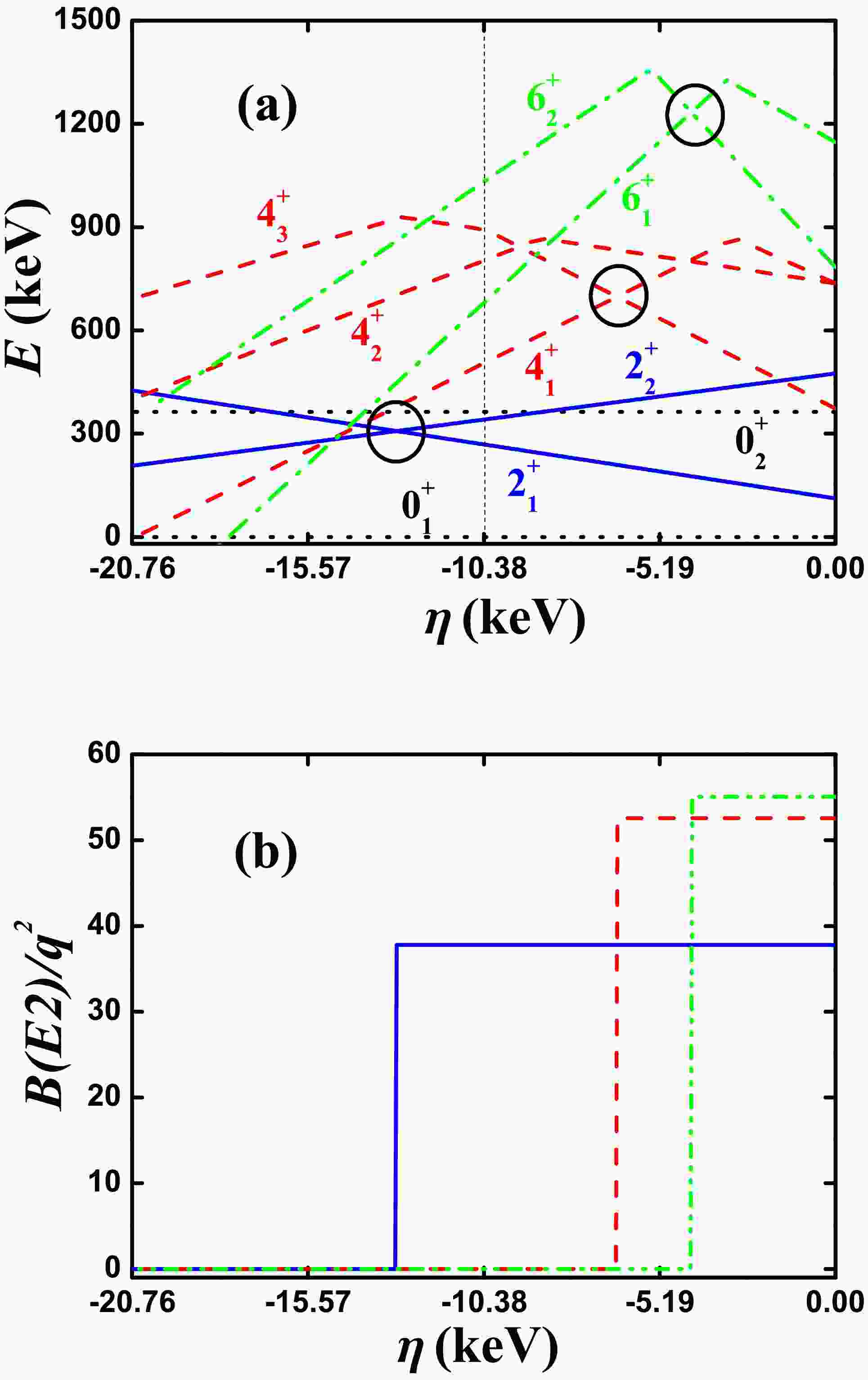
Now we discuss the first example using SU(3) analysis. Fig. 1(a) shows the evolutional behaviors of the partial low-lying levels as a function of η in the SU(3) symmetry limit in Ref. [40]. This is the first successful explanation for the B(E2) anomaly of realistic nucleus $ ^{170} {\rm{Os}}$. The boson number is $ N = 9 $. In [40], the parameters are $ \alpha = 302.4 $ keV, $ \beta = -30.09 $ keV, $ \gamma = 3.79 $ keV, $ \delta = 0.0 $ keV, $ \eta = -10.38 $ keV, $ \zeta = 0.0 $ keV and $ \xi = 18.66 $ keV. For SU(3) analysis, let $ \alpha = 0 $. The ground state is a prolate shape with SU(3) irrep (18,0). In that paper, the two SU(3) third-order interactions are considered, but the two four-order interactions are not. From Fig. 1(a), we can see, when η varies from 0 to -20.76 keV (the middle point $ \eta = -10.38 $ keV is the parameter used in [40]), the red dashed line of the $ 4_{1}^{+} $ state can intersect with the one of one other $ 4^{+} $ state at $ \eta = -6.45 $ keV (the crossover point is marked by the black circle, and the latter ones are also the same). In [40], it is known that the $ 4^{+} $ state in the SU(3) irrep (10,4) becomes lower than the $ 4^{+} $ state in the SU(3) irrep (18,0). In Fig. 1(a), we can also notice some new features that are not observed by previous studies. The $ 6_{1}^{+} $ state can intersect with one other $ 6^{+} $ state at $ \eta = -4.25 $ keV (the green dashed dotted lines) and importantly, the $ 2_{1}^{+} $ state can intersect with one other $ 2^{+} $ state at $ \eta = -12.97 $ keV (the blue real lines) (all marked by the black circles). Thus some new results are directly found.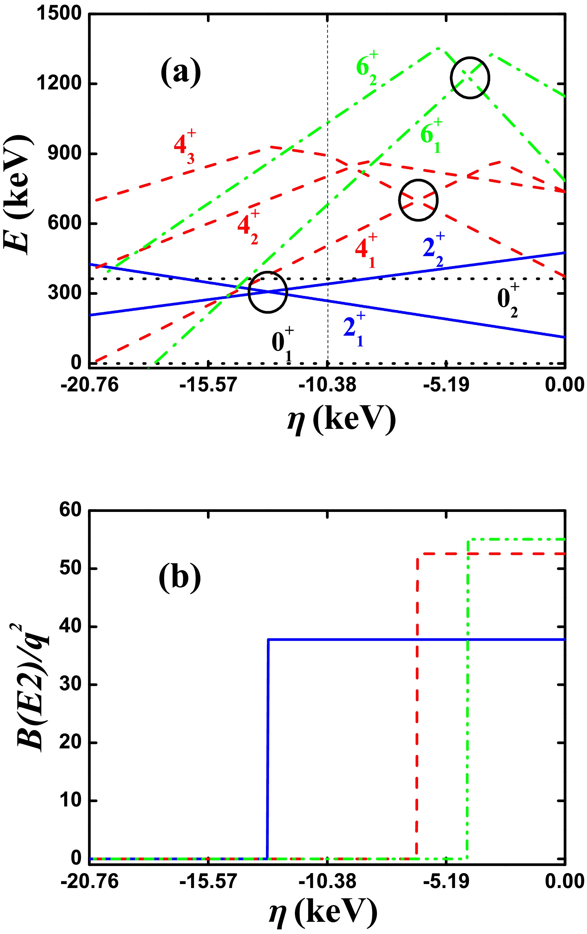

Figure 1.  (color online) (a) The evolutional behaviors of the partial low-lying levels as a function of η; (b) The evolutional behaviors of the $ B(E2; 2_{1}^{+}\rightarrow 0_{1}^{+}) $ (blue real line), $ B(E2; 4_{1}^{+}\rightarrow 2_{1}^{+}) $ (red dashed line), $ B(E2; 6_{1}^{+}\rightarrow 4_{1}^{+}) $ (green dashed dotted line) as a function of η. The parameters are deduced from [40].

A key question, which has been noticed but not highlighted in previous studies, is that the new energy spectra still appear to be in order and are very similar to the conventional ones. If put the four nuclei $ ^{172} {\rm{Pt}}$, $ ^{168,170} {\rm{Os}}$ and $ ^{166} {\rm{W}}$ with B(E2) anomaly into the entire isotopic evolutions, see [19−22], it looks very natural, but the B(E2) values suddenly change. An imperceptible change has occurred. Here we emphasize this point. At the thin dashed line in the middle ($ \eta = -10.38 $ keV) in Fig. 1(a) the energy spectra in the SU(3) symmetry limit discussed in Ref. [40] are presented. It can be seen that although level-crossing occurs, the positions of the energy levels does not change too much (compared with the ones at $ \eta = 0 $). Unless the selected parameter is too large, the energy levels are still in order. If the $ \hat{n}_{d} $ interaction is added, the changes can be more smaller. This approximate mirror effect is very interesting, and will be discussed in future.

In the SU(3) symmetry limit, if two states belong to different SU(3) irreps., the E2 transitions between them must be 0. In Fig. 1(b), the evolutional behaviors of the $ B(E2; 2_{1}^{+}\rightarrow 0_{1}^{+}) $, $ B(E2; 4_{1}^{+}\rightarrow 2_{1}^{+}) $, $ B(E2; 6_{1}^{+}\rightarrow 4_{1}^{+}) $ as a function of η are shown. We can see $ B(E2; 4_{1}^{+}\rightarrow 2_{1}^{+}) $ anomaly (here anomaly means the E2 transition is 0) can appear when $ \eta\leq -6.45 $ keV, and we can also notice that $ B(E2; 6_{1}^{+}\rightarrow 4_{1}^{+}) $ anomaly can happen when $ \eta\leq -4.25 $ keV and $ B(E2; 2_{1}^{+}\rightarrow 0_{1}^{+}) $ anomaly can occur when $ \eta\leq -12.97 $ keV. These anomalies are not mentioned in previous studies, and importantly we find they really exist in realistic nuclei, such as $ B(E2; 6_{1}^{+}\rightarrow 4_{1}^{+}) $ anomaly for $ ^{72} {\rm{Zn}}$ [29] and $ B(E2; 2_{1}^{+}\rightarrow 0_{1}^{+}) $ anomaly for $ ^{166} {\rm{Os}}$ [58]. We believe that the $ B(E2; 2_{1}^{+}\rightarrow 0_{1}^{+}) $ anomaly in $ ^{166} {\rm{Os}}$ is critical for understanding the reason of the B(E2) anomaly in realistic nuclei. The $ B(E2; 2_{1}^{+}\rightarrow 0_{1}^{+}) $ anomaly in $ ^{166} {\rm{Os}}$ has been discussed with a general explanatory framework [59].

Clearly SU(3) analysis is a powerful technique to understand the B(E2) anomaly. Due to within the SU(3) symmetry limit, the level-crossing phenomena can occur which is induced by the $ [L\times Q \times L]^{(0)} $ interaction. If the two levels belong to different SU(3) irrep., the E2 transition must be 0. This case is different from the SU(3) corresponding of the rigid triaxial description found in [60].

Ref. [41] continued the rigid triaxial description. Here we use $ ^{168} {\rm{Os}}$ for SU(3) analysis. The SU(3) corresponding of the rigid triaxial description was found in [61−63], then it was used in the IBM to remove the degeneracy of the β and γ bands [64] and to describe the rigid triaxial spectra [65]. A key step is that Ref. [50] discussed the extended cubic Q-consistent Hamiltonian and found a new evolutional path from the prolate shape to the oblate shape. This asymmetric shape evolution was also studied analytically in [51]. Ref. [60] first found the B(E2) anomaly theoretically in studying the rigid triaxial rotor. Unfortunately, they don't realize that realistic nuclei can really show such features in that paper. The feature in [60] is that, when the angular moment L in the ground band increases, the E2 transitional values $ B(E2; L_{1}^{+}\rightarrow (L-2)_{1}^{+}) $ really decrease, but at the beginning it decreases slowly, that $ B_{4/2}>0.5 $.

For $ ^{168} {\rm{Os}}$, the boson number is $ N = 8 $. The parameters in Fig. 2 deduced from [41] are $ \alpha = 22 $ keV, $ \beta = 96 $ keV, $ \gamma = 27 $ keV, $ \delta = 0.3 $ keV, $ \eta = 53 $ keV, $ \zeta = -45 $ keV and $ \xi = 94 $ keV. For SU(3) analysis, let $ \alpha = 0 $. Fig. 2(a) shows the evolutional behaviors of the partial low-lying levels as a function of η from 0 to 106 keV, and the middle point is the parameter in [41] ($ \eta = 53 $ keV). Obviously, the $ 4_{1}^{+} $ state really can not intersect with other $ 4^{+} $ states (the red dashed lines), but we can see that the $ 6_{1}^{+} $ state intersects with one other $ 6^{+} $ state (the green dashed dotted lines and see the black circle). As shown in Fig. 2(b), the $ B(E2; 4_{1}^{+}\rightarrow 2_{1}^{+}) $ value can be lower than the $ B(E2; 2_{1}^{+}\rightarrow 0_{1}^{+}) $ value, so the B(E2) anomaly exists and results from the rigid triaxial rotor effect. However this ratio $ B_{4/2} $ is 0.6 at the middle point, larger than the experimental value 0.34. Whether the rigid triaxial rotor effect can provide such a small $ B_{4/2} $ value is a problem, which should be studied in future. Clearly, the $ B(E2; 6_{1}^{+}\rightarrow 4_{1}^{+}) $ anomaly results from the level-crossing effect. Here the SU(3) irrep of the ground state is (4,6) ($ \gamma = 35.6^{\circ} $ according to equating (7)), thus the B(E2) values are smaller than the ones in Fig. 1(b) if they exist. Recently, Ref. [47, 48] found that, the small B(E2) anomaly can be found for the rigid triaxial rotor in the IBM-2 which distinguishes the protons and neutrons. In the SU3-IBM, the protons and neutrons can be also distinguished and more complicated mechanisms can be found for the B(E2) anomaly.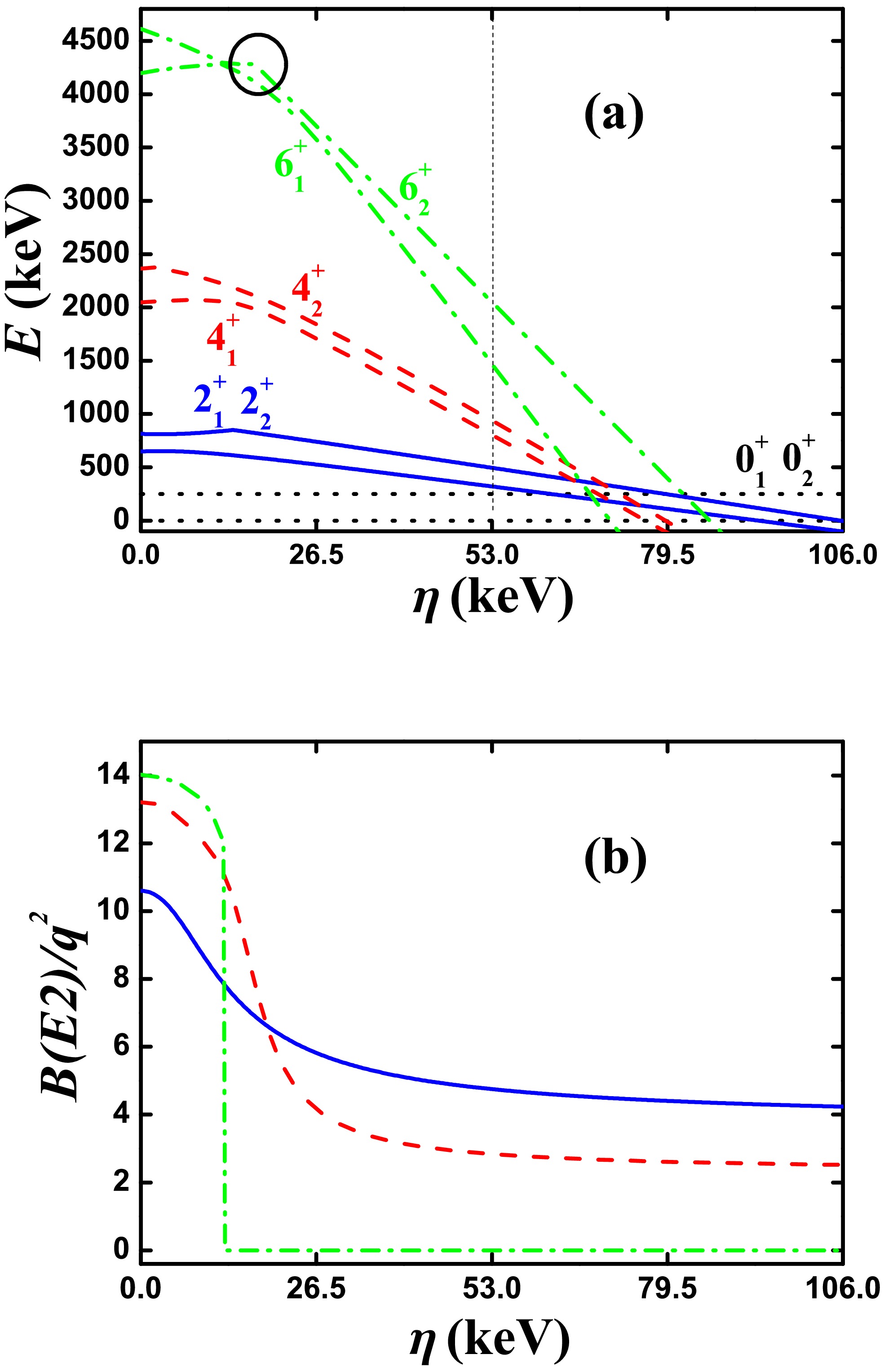

Figure 2.  (color online) (a) The evolutional behaviors of the partial low-lying levels as a function of η; (b) The evolutional behaviors of the $ B(E2; 2_{1}^{+}\rightarrow 0_{1}^{+}) $ (blue real line), $ B(E2; 4_{1}^{+}\rightarrow 2_{1}^{+}) $ (red dashed line), $ B(E2; 6_{1}^{+}\rightarrow 4_{1}^{+}) $ (green dashed dotted line) as a function of η. The parameters are deduced from [41].

In [41], there are another group of parameters for $ ^{168} {\rm{Os}}$, which are $ \alpha = 99 $ keV, $ \beta = 50.4 $ keV, $ \gamma = 3.5 $ keV, $ \delta = 0.55 $ keV, $ \eta = 43 $ keV, $ \zeta = -9.7 $ keV and $ \xi = 26 $ keV. For SU(3) analysis, let $ \alpha = 0 $. Fig. 3(a) shows the evolutional behaviors of the partial low-lying levels as a function of η from 0 to 86 keV, and the middle point is the parameter in [41] ($ \eta = 43 $ keV). Obviously, the $ 4_{1}^{+} $ state intersects with one other $ 4^{+} $ state at $ \eta = 23 $ keV (the red dashed lines) and the $ 6_{1}^{+} $ state intersects with one other $ 6^{+} $ state at $ \eta = 30.1 $ keV (the green dashed dotted lines), which is larger than the one of the $ 4^{+} $ states crossing point (see the two black circles). Thus this B(E2) anomaly results from level-crossing effect. However these crossing effects may be very complicated. Thus confirming the actual crossing effects of the experimental results requires more experimental data. If so, the emergence of the B(E2) anomaly may be an accidental effect. In Fig. 3(b) the $ B(E2; 4_{1}^{+}\rightarrow 2_{1}^{+}) $ anomaly and the $ B(E2; 6_{1}^{+}\rightarrow 4_{1}^{+}) $ anomaly can occur simultaneously. Here the SU(3) irrep of the ground state is (2,4) ($ \gamma = 35.8^{\circ} $ according to (7)), so the B(E2) values becomes smaller if they exist.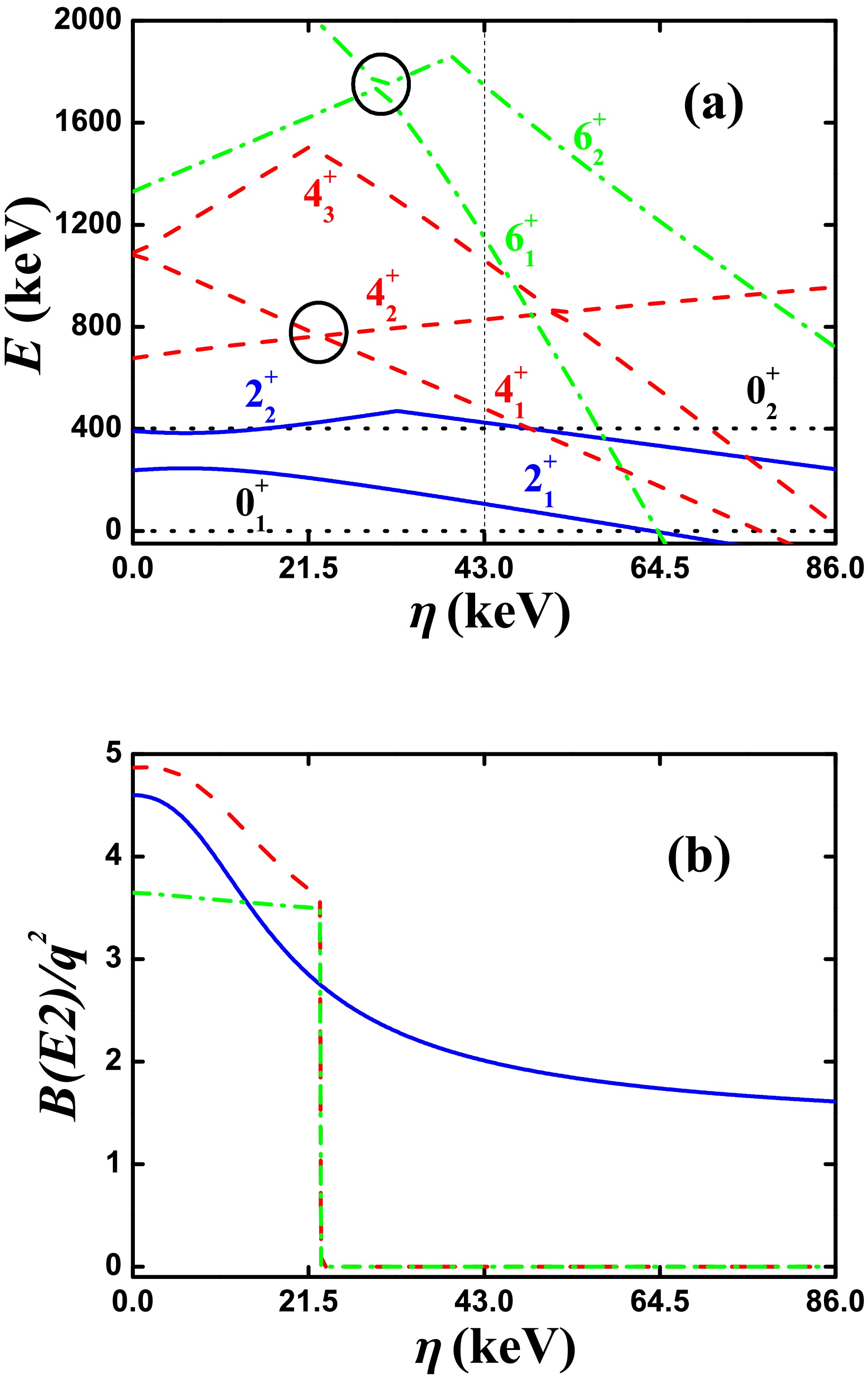

Figure 3.  (color online) (a) The evolutional behaviors of the partial low-lying levels as a function of η; (b) The evolutional behaviors of the $ B(E2; 2_{1}^{+}\rightarrow 0_{1}^{+}) $ (blue real line), $ B(E2; 4_{1}^{+}\rightarrow 2_{1}^{+}) $ (red dashed line), $ B(E2; 6_{1}^{+}\rightarrow 4_{1}^{+}) $ (green dashed dotted line) as a function of η. The parameters are deduced from [41].

When discussing the B(E2) anomaly, not only the ratio $ B_{4/2} $, but also the absolute value of $ B(E2;2_{1}^{+}\rightarrow 0_{1}^{+}) $ should be also considered. If place the four nuclei $ ^{172} {\rm{Pt}}$, $ ^{168,170} {\rm{Os}}$ and $ ^{166} {\rm{W}}$ with B(E2) anomaly in the isotopic evolutions [19−22], these results vary continuously. This is also the key for considering these spectra as the collective excitation. Too small $ B(E2;2_{1}^{+}\rightarrow 0_{1}^{+}) $ value implies a large effective charge q, which may not be very reasonable, see [52].

In previous IBM, O(5) symmetry exists when evolving from the U(5) limit to the O(6) limit, which results in the crossover of the $ 0_{2}^{+} $ and $ 0_{3}^{+} $ states. When the parameters deviate a little, significant energy level exclusion can occur [18]. No doubt this is important to confirm such phenomena. Recently in the SU3-IBM, similar result was also found in [54], which is a level-anticrossing phenomenon.

Some important new results has been obtained recently. In [44], the SU(3) quadrupole operator $ \hat{Q} $ is replaced by the generalised quadrupole operator $ \hat{Q}_{\chi} $. We also take the $ ^{168} {\rm{Os}}$ as an example, where $ \alpha = 0 $, and other parameters are $ \beta = -25.0 $ keV, $ \gamma = 0 $, $ \delta = 0 $, $ \eta = -26.9 $ keV, $ \zeta = 0 $ and $ \xi = 43.65 $ keV and $ \chi = -0.39 $. For SU(3) analysis, let $ \chi = -\frac{\sqrt{7}}{2} $. Here the SU(3) irrep of the ground state is (16,0) with the prolate shape. Fig. 4(a) shows the evolutional behaviors of the partial low-lying levels as a function of η from 0 to -53.8 keV, and the middle point is the parameter in [44] ($ \eta = -26.9 $ keV). Intuitively, this evolutional behavior is very similar to the ones in Fig. 1(a). The $ 4_{1}^{+} $ state intersects with one other $ 4^{+} $ state at $ \eta = -44.8 $ keV (the red dashed lines), and the $ 6_{1}^{+} $ state also intersects with one other $ 6^{+} $ state at $ \eta = -29.4 $ keV (the green dashed dotted lines). The two crossover points are marked by the black circles. It implies that this B(E2) anomaly is also related to the SU(3) symmetry.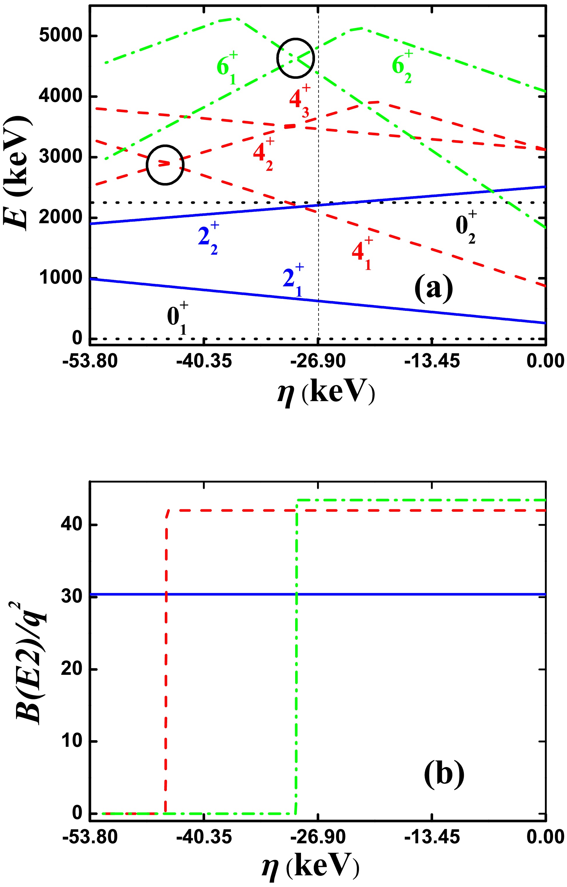

Figure 4.  (color online) (a) The evolutional behaviors of the partial low-lying levels as a function of η; (b) The evolutional behaviors of the $ B(E2; 2_{1}^{+}\rightarrow 0_{1}^{+}) $ (blue real line), $ B(E2; 4_{1}^{+}\rightarrow 2_{1}^{+}) $ (red dashed line), $ B(E2; 6_{1}^{+}\rightarrow 4_{1}^{+}) $ (green dashed dotted line) as a function of η. The parameters are deduced from [44].

We can notice that, the middle point shows a normal $ B_{4/2} $ value, but it is near the anomalous region. This is very interesting, and gives a new mechanism for B(E2) anomaly, which is related with the level-anticrossing phenomenon. In [66], this new new mechanism is discussed in detail, and it is found that the B(E2) anomaly in the SU(3) symmetry limit and the B(E2) anomaly along the transitional region from the SU(3) symmetry limit to the O(6) symmetry limit are closely related. These results can help us to further explain the anomalous small $ B(E2;2_{1}^{+}\rightarrow 0_{1}^{+}) $ value in $ ^{166} {\rm{Os}}$ [59].

A reasonable theory is not only to explain the small $ B_{4/2} $ values, but also to consider the normal $ B(E2;2_{1}^{+}\rightarrow 0_{1}^{+}) $ values in $ ^{172} {\rm{Pt}}$, $ ^{168,170} {\rm{Os}}$ and $ ^{166} {\rm{W}}$, and to explain the anomalous small $ B(E2;2_{1}^{+}\rightarrow 0_{1}^{+}) $ value in $ ^{166} {\rm{Os}}$ [58]. These will be discussed in [59].

Ref. [46] found a new mechanism at the oblate side. We also take $ ^{168} {\rm{Os}}$ for an example, where $ \alpha = 72.0 $ keV, $ \beta = -7.825 $ keV, $ \gamma = 2.636 $ keV, $ \delta = 0 $, $ \eta = 15.1 $ keV, $ \zeta = -1.09 $ keV and $ \xi = 36.87 $ keV. For SU(3) analysis, let $ \alpha = 0 $. Here the SU(3) irrep of the ground state is (0,8) with the oblate shape. Fig. 5(a) shows the evolutional behaviors of the partial low-lying levels as a function of η from 0 to 30.2 keV, and the middle point is the parameter in [46] ($ \eta = 15.1 $ keV). We can see that the $ 2_{1}^{+} $ and $ 2_{2}^{+} $ states intersects with each other at $ \eta = 12.1 $ keV (the blue real lines), the $ 4_{1}^{+} $ and $ 4_{2}^{+} $ states intersects with each other at $ \eta = 4.6 $ keV (the red dashed lines), and the $ 6_{1}^{+} $ and $ 6_{2}^{+} $ states at $ \eta = 2.5 $ keV (the green dashed dotted lines). The three crossover points are marked by the black circles. At the middle point, the $ B_{4/2} $ value is infinity. This is very interesting. We can also confirm that this B(E2) anomaly is related to the SU(3) symmetry. This new mechanism will be discussed in section V in detail.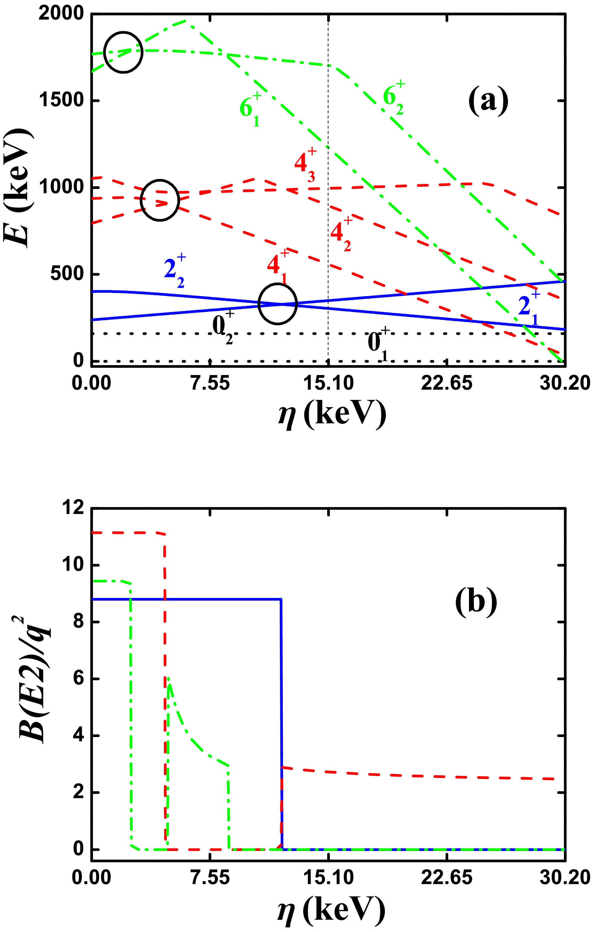

Figure 5.  (color online) (a) The evolutional behaviors of the partial low-lying levels as a function of η; (b) The evolutional behaviors of the $ B(E2; 2_{1}^{+}\rightarrow 0_{1}^{+}) $ (blue real line), $ B(E2; 4_{1}^{+}\rightarrow 2_{1}^{+}) $ (red dashed line), $ B(E2; 6_{1}^{+}\rightarrow 4_{1}^{+}) $ (green dashed dotted line) as a function of η. The parameters are deduced from [46].

These results in the five examples broaden our understanding of the B(E2) anomaly. Even the conditions, that (1) the $ B(E2; 2_{1}^{+}\rightarrow 0_{1}^{+}) $ value exists and (2) the $ B(E2; 4_{1}^{+}\rightarrow 2_{1}^{+}) $ is 0, are not satisfied in the SU(3) symmetry limit, the B(E2) anomaly can also appear.

If an explanation for B(E2) anomaly can have a SU(3) symmetry limit, the SU(3) analysis should be performed. From the above examples from [40−47], we can get many new results. There are some phenomena that seem to have nothing to do with the SU(3) symmetry, but are actually related to do with it. This may be a more complicated mechanism, which we need to further elaborate on in [66]. In the SU(3) analysis, if any level-crossing can not occur but the B(E2) anomaly can happen, it can be considered from the rigid triaxial rotor effect. If any B(E2) anomaly does not exist in the SU(3) analysis but the B(E2) anomaly can happen when the d boson number operator is added (this is almost impossible) or the $ \hat{Q} $ is replaced by the $ \hat{Q}_{\chi} $, this will be very important. A general discussion will be given in future with the extended Q-consistent Hamiltonian with up to fourth-order interactions. In a previous paper [38], it has been proved that, in this extended Hamiltonian, when $ \chi = 0 $, that is the O(6) symmetry limit, the B(E2) anomaly can not happen. Thus it is important to discuss the evolving region from the SU(3) symmetry limit to the O(6) symmetry limit.

For the first and fourth examples, the parameters η of the fourth-order interactions $ [(\hat{L}\times \hat{Q})^{(1)} \times (\hat{L} \times \hat{Q})^{(1)}]^{(0)} $ are 0. Thus the evolutional behaviors of the B(E2) values in Fig. 1(b) and 4(b) are simple. When this interactions is added, more complex evolutional behaviors can be observed, which is very interesting. Although this interaction has been studied in the rigid triaxial explanation [41, 46, 47, 60], many details are also inadequate. For the second and third examples, the sigh of η is negative, and the evolutional behaviors of the B(E2) values in Fig. 2(b) and 3(b) becomes more complex (the evolution lines become curved), but sill similar to the cases in Fig. 1(b) and Fig. 4(b). However for the fifth example, the sigh of η is positive, and the evolutional behaviors of the B(E2) values in Fig. 5(b) becomes more complex than the ones in Fig. 2(b) and Fig. 3(b). Thus further discussing the $ [(\hat{L}\times \hat{Q})^{(1)} \times (\hat{L} \times \hat{Q})^{(1)}]^{(0)} $ interaction is necessary to understand the more complex B(E2) anomaly, such as in $ ^{72,74} {\rm{Zn}}$ [29−31] and $ ^{114} {\rm{Te}}$ [32, 33].

In this section, we further discuss the new mechanism in Fig. 5 [46]. In Fig. 5(b), the changes of the values of $ B(E2; 2_{1}^{+}\rightarrow 0_{1}^{+}) $ (blue real line), $ B(E2; 4_{1}^{+}\rightarrow 2_{1}^{+}) $ (red dashed line), $ B(E2; 6_{1}^{+}\rightarrow 4_{1}^{+}) $ (green dashed dotted line) are similar to the ones in Fig. 1(b), but shows more complicated behaviors. The key for this is the introduction of the fourth-order interaction $ [(\hat{L}\times \hat{Q})^{(1)} \times (\hat{L} \times \hat{Q})^{(1)}]^{(0)} $. The effect of the SU(3) fourth-order interactions on the B(E2) anomaly is very complex, and the detailed discussion will be given in future. Here, just the parameters in [46] are used. We can see that the fourth-order interaction brings in some new features.

In Fig. 5(b), when $ \eta = 15.1 $ keV (the parameter used in [46]), $ B(E2; 2_{1}^{+}\rightarrow 0_{1}^{+}) = 0 $ while $ B(E2; 4_{1}^{+}\rightarrow 2_{1}^{+})\neq 0 $. Thus $ B_{4/2} = \infty $, which is a new result. When $ \eta = 11.325 $ keV, $ B(E2; 2_{1}^{+}\rightarrow 0_{1}^{+})\neq0 $ while $ B(E2; 4_{1}^{+}\rightarrow 2_{1}^{+}) = 0 $. Thus $ B_{4/2} = 0 $, which has been discovered before. For both cases, $ B(E2; 6_{1}^{+}\rightarrow 4_{1}^{+}) = 0 $. When $ \eta = 7.55 $ keV, $ B(E2; 2_{1}^{+}\rightarrow 0_{1}^{+})\neq 0 $, $ B(E2; 4_{1}^{+}\rightarrow 2_{1}^{+}) = 0 $ while $ B(E2; 6_{1}^{+}\rightarrow 4_{1}^{+})\neq 0 $. When the fourth-order interaction is introduced, any B(E2) results may be obtained.

Fig. 6 − 8(a) present the evolutional behaviors of the partial low-lying levels as a function of α from 0 to 200 keV when $ \eta = 15.1 $ keV, 11.325 keV and 7.55 keV. The evolutional trends are similar. Fig. 6 − 8(b) show the evolutional behaviors of the values of $ B(E2; 2_{1}^{+}\rightarrow 0_{1}^{+}) $, $ B(E2; 4_{1}^{+}\rightarrow 2_{1}^{+}) $, $ B(E2; 6_{1}^{+}\rightarrow 4_{1}^{+}) $ as a function of α when $ \eta = 15.1 $ keV, 11.325 keV and 7.55 keV. The evolutional trends look very different.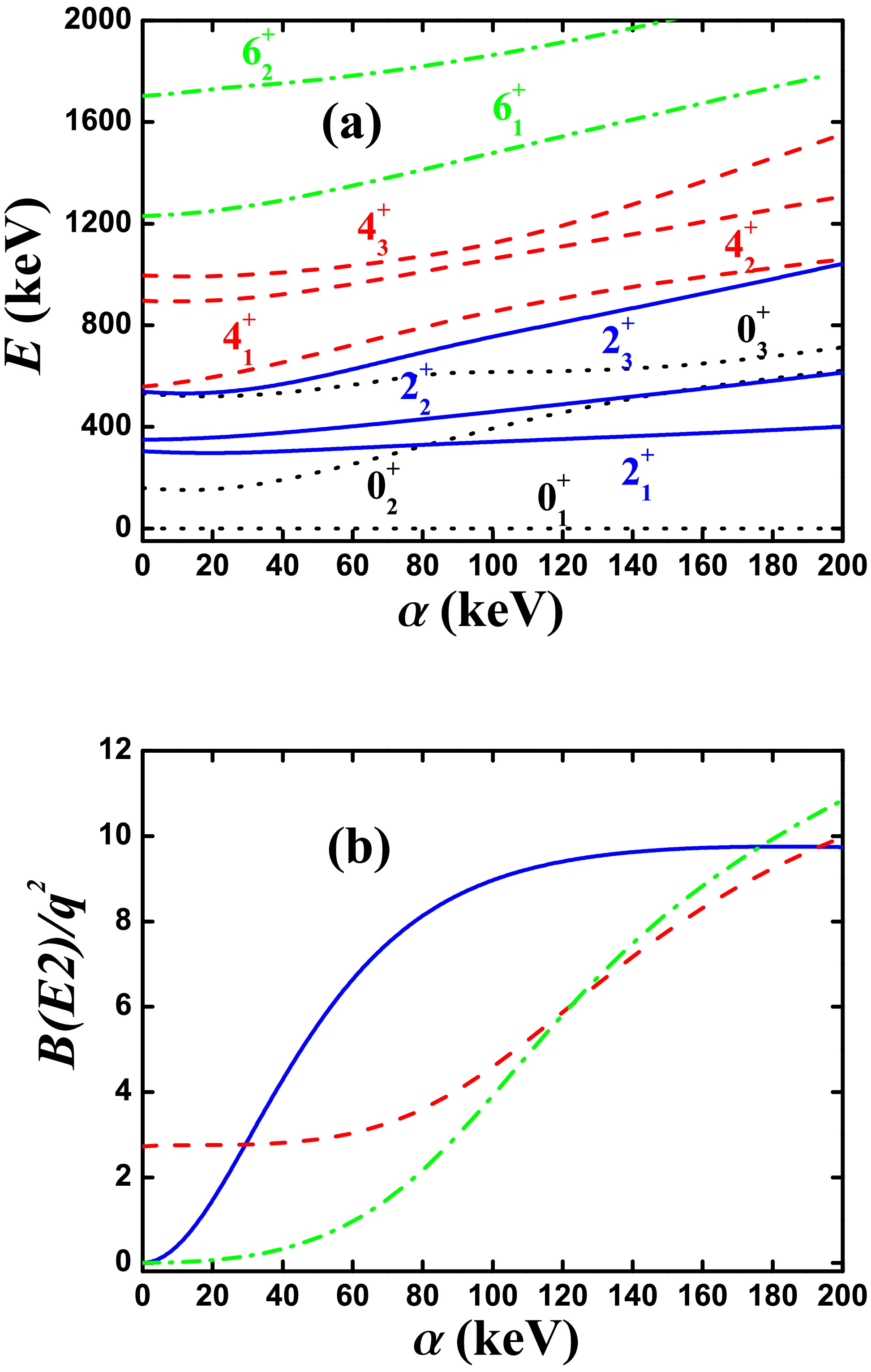

Figure 6.  (color online) (a) The evolutional behaviors of the partial low-lying levels as a function of α; (b) The evolutional behaviors of the $B(E2; 2_{1}^{+}\rightarrow 0_{1}^{+})$ (blue real line), $B(E2; 4_{1}^{+}\rightarrow 2_{1}^{+})$ (red dashed line), $B(E2; 6_{1}^{+}\rightarrow 4_{1}^{+})$ (green dashed dotted line) as a function of α. The parameters are deduced from [46] ($\eta=15.1$ keV).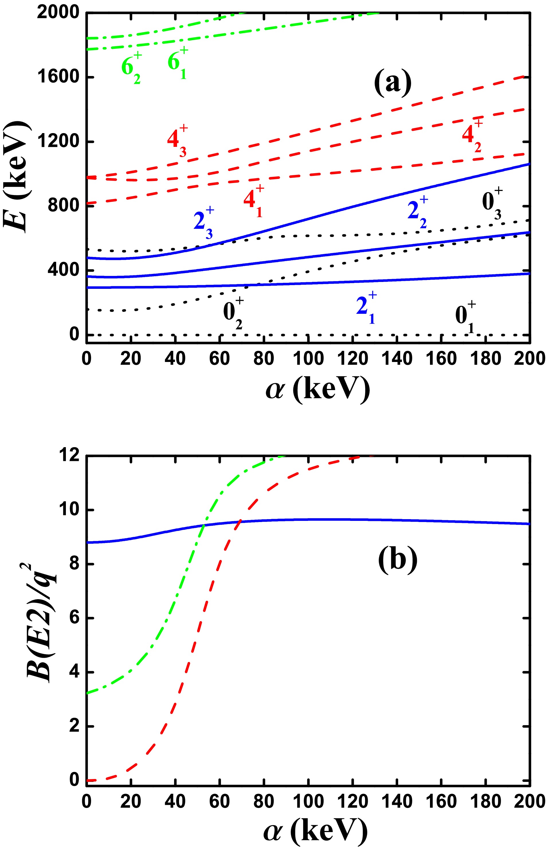

Figure 8.  (a) The evolutional behaviors of the partial low-lying levels as a function of α; (b) The evolutional behaviors of the $B(E2; 2_{1}^{+}\rightarrow 0_{1}^{+})$ (blue real line), $B(E2; 4_{1}^{+}\rightarrow 2_{1}^{+})$ (red dashed line), $B(E2; 6_{1}^{+}\rightarrow 4_{1}^{+})$ (green dashed dotted line) as a function of α. The parameters are deduced from [46] but $\eta=7.55$ keV.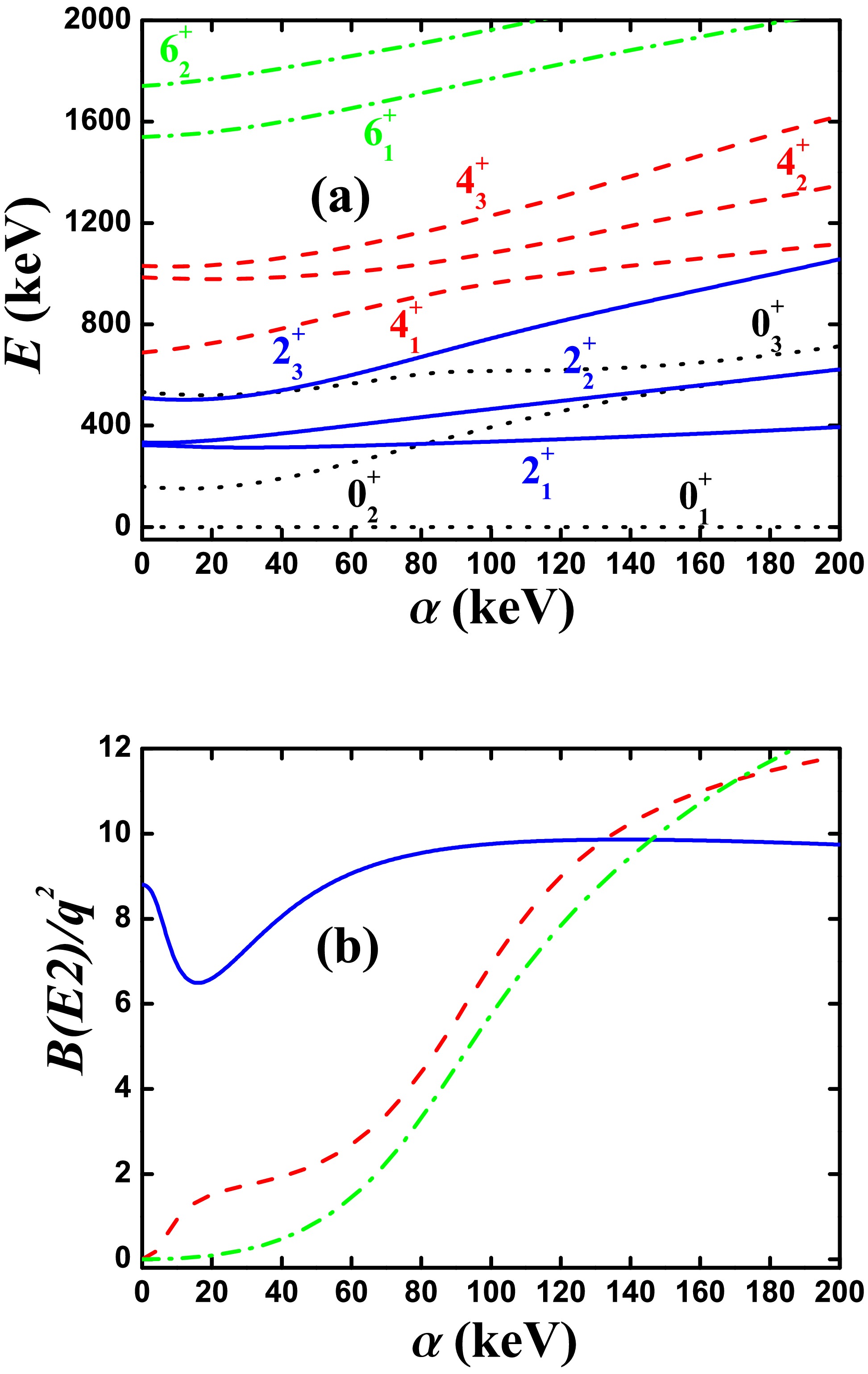

Figure 7.  (color online) (a) The evolutional behaviors of the partial low-lying levels as a function of α; (b) The evolutional behaviors of the $B(E2; 2_{1}^{+}\rightarrow 0_{1}^{+})$ (blue real line), $B(E2; 4_{1}^{+}\rightarrow 2_{1}^{+})$ (red dashed line), $B(E2; 6_{1}^{+}\rightarrow 4_{1}^{+})$ (green dashed dotted line) as a function of α. The parameters are deduced from [46] but $\eta=11.325$ keV.

Fig. 9 presents the evolutional behaviors of the $ B_{4/2} $ values as a function of α for $ \eta = 15.1 $ keV, $ \eta = 11.325 $ keV and $ \eta = 7.55 $ keV. Other parameters are deduced from [46]. In $ ^{168} {\rm{Os}}$, $ B_{4/2} = 0.34 $. For $ \eta = 15.1 $ keV, the smallest value is 0.45. In [46], $ B_{4/2} = 0.53 $ was used. In next section, $ B_{4/2} = 0.45 $ is used for result 1 (black point). For $ \eta = 11.325 $ keV and 7.55 keV, $ B_{4/2} = 0.34 $ exist (blue point and red point) and are used for result 2 and result 3. For comparison, $ B_{4/2} = 0 $ is also used for result 4 when $ \eta = 7.55 $ keV, which is just the SU(3) analysis of result 3.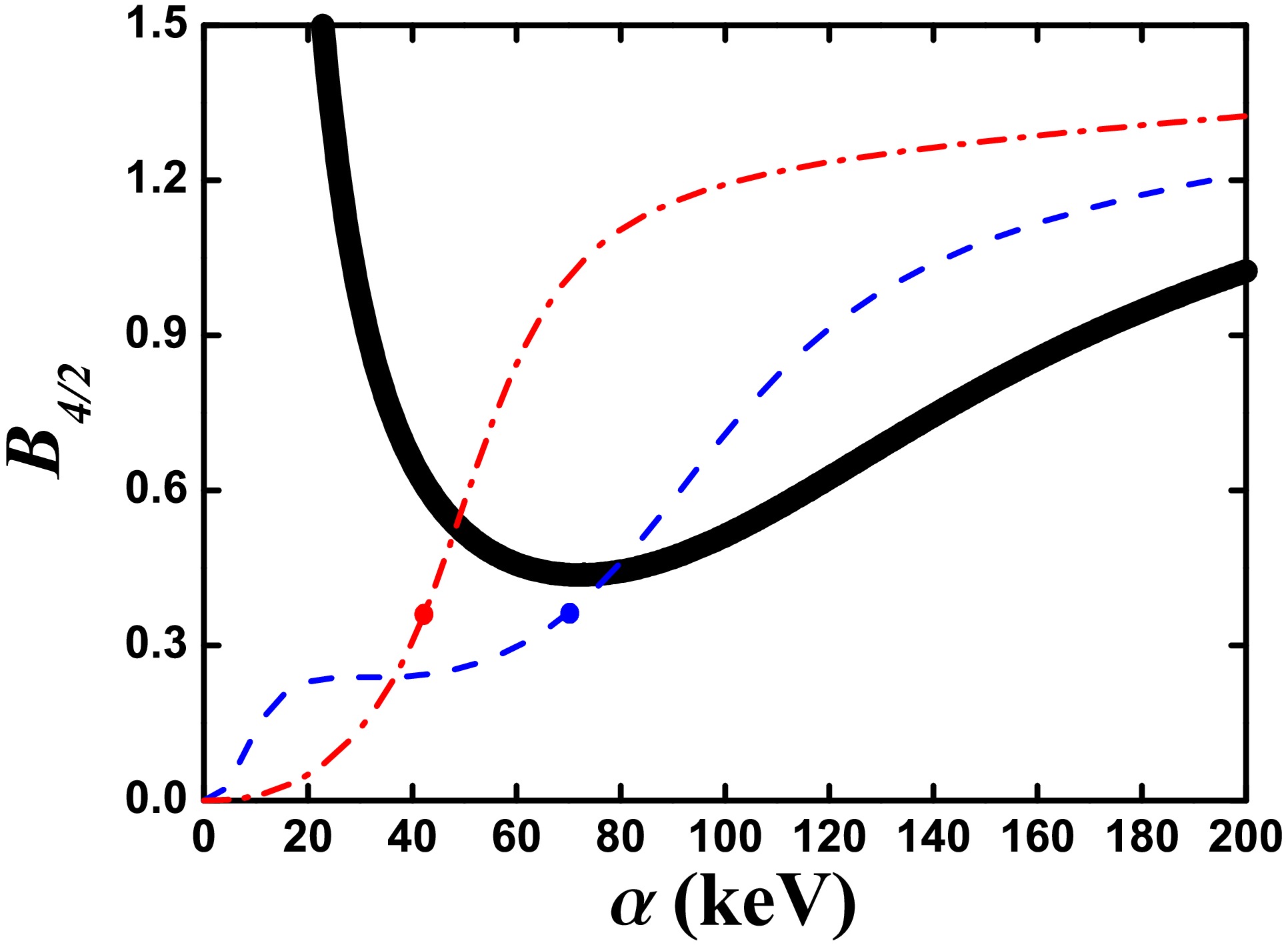

Figure 9.  The evolutional behaviors of the $ B_{4/2} $ values as a function of α for $ \eta = 15.1 $ keV (black real line), $ \eta = 11.325 $ keV (blue dashed dotted line) and $ \eta = 7.55 $ keV (red dashed dotted line). Other parameters are deduced from [46].

If the fourth-order interaction $ [(\hat{L}\times \hat{Q})^{(1)} \times (\hat{L} \times \hat{Q})^{(1)}]^{(0)} $ is not added, the B(E2) values of each energy level in the yrast band can gradually decrease as the angular momentum L increases [40, 60]. However when this interaction is added, this change can become more irregular. This is important for understanding some irregular B(E2) anomalies.

Result $ 1-3 $ correspond to the three points (black, blue and red) in Fig. 9. Result 4 corresponds to the $ \alpha = 0 $ point of the red line in Fig. 9. Let the energy of the $ 2_{1}^{+} $ state be equal to the experimental one in $ ^{168} {\rm{Os}}$. Parameters of the four results are shown in Table 1 and the fitting values are shown in Table 2. For result 1, 2 and 3, the energies of the $ 0_{2}^{+} $ state and $ 2_{2}^{+} $ state increase. For result 1 and 2, the values of $ B(E2; 8_{1}^{+}\rightarrow 6_{1}^{+}) $ are larger. For result 3, the value of $ B(E2; 6_{1}^{+}\rightarrow 4_{1}^{+}) $ is larger. Thus these B(E2) values are sensitive to the parameters. For result 4, the results of the SU(3) analysis are shown. The irregular B(E2) values are clear when L increases. When $ \hat{n}_{d} $ is added, the result 4 becomes the result 3, which has the better fitting effect. Level-crossing is indeed a possible reason for the emergence of the B(E2) anomaly. For a better understanding of the B(E2) anomaly in $ ^{168} {\rm{Os}}$, more experimental results are needed.

	Exp.	Res. 1	Res. 2	Res. 3	Res. 4
$ E_{2_{1}^{+}} $	341	341	341	341	341
$ E_{4_{1}^{+}} $	857	857	857	867	857
$ E_{6_{1}^{+}} $	1499	1607	1586	1642	1898
$ E_{8_{1}^{+}} $	2223	2342	2136	2103	2771
$ E_{10_{1}^{+}} $	2983	3522	3248	2960	4213
$ E_{0_{2}^{+}} $		261	380	521	276
$ E_{2_{2}^{+}} $		424	463	575	461
$ E_{3_{1}^{+}} $		778	821	962	841
$ E_{4_{2}^{+}} $		1057	1055	1064	1130
$ B(E2;2^{+}_{1}\rightarrow 0^{+}_{1}) $	74(13)	74	74	74	74
$ B(E2;4^{+}_{1}\rightarrow 2^{+}_{1}) $	25(13)	33	25	25	0
$ B(E2;6^{+}_{1}\rightarrow 4^{+}_{1}) $		16	16	50	27
$ B(E2;8^{+}_{1}\rightarrow 6^{+}_{1}) $		57	49	11	0
$ B(E2;10^{+}_{1}\rightarrow 8^{+}_{1}) $		2.8	2.8	22	14

Table 2.  Experimental values and fitting values of the four results for $ ^{168} $Os. The unit of the energy of the energy level is keV and the unit of the B(E2) value is W.u.. The effective charges of results 1-4 are 3.114 $ \sqrt{ \rm{W.u.}} $, 2.2825 $ \sqrt{ \rm{W.u.}} $, 2.823 $ \sqrt{ \rm{W.u.}} $ and 2.900 $ \sqrt{ \rm{W.u.}} $ respectively.

In this paper, we propose a powerful technique for understanding the B(E2) anomaly. It is the SU(3) analysis. From the discussions of the examples in [40−47], many new results are obtained. There are three of the most important ones. First, the SU(3) third-order interaction $ [L\times Q \times L]^{(0)} $ is critical for the SU(3) anomaly. Whether this relationship is unique requires further investigation. Second, when this interaction is added, various level-crossing phenomena can happen. The causes of the B(E2) anomaly in realistic experiments require more experimental researches to determine. Looking for more mechanisms for the B(E2) anomaly also seems to be needed. Third, not only the value of $ B(E2;4_{1}^{+}\rightarrow 2_{1}^{+}) $ but also the $ B(E2;6_{1}^{+}\rightarrow 4_{1}^{+}) $ and $ B(E2;2_{1}^{+}\rightarrow 0_{1}^{+}) $ can be anomalous. The B(E2) anomaly in $ ^{168} {\rm{Os}}$ is discussed. It is very important to find more and more B(E2) anomaly results in the experiments.