Thermal analysis and Joule-Thomson expansion of black hole exhibiting metric-affine gravity

One of the most attractive and challenging subjects of study is the geometrical structure of black hole (BH) in general relativity (GR) and modified theories of gravity [1]. The thermal characteristics of BHs and their behavior are analyzed by well-known four laws of BH mechanics [2, 3]. After that the work of Bekenstein, first-time Stephen Hawking presented the existence of BH radiations and formalized the tunneling process very near the BH horizon due to the vacuum fluctuations. It is observed that the small amount of heat quantity leads to the eccentricity of quantum mechanics [4, 5]. In the literature [6], it is noted that the BHs contain thermodynamic features like temperature and entropy. At the BH horizon, the Hawking temperature is proportional to its surface gravity due to BH behaves like a thermodynamical system. It is certified that results of [7] are useful to all classical BHs at thermodynamic equilibrium.

The Hawking temperature phase transition takes place after the justification of a phase structure isomorphic associated with the Van der Waals liquid-gas system in Kerr RN-AdS BH [8] and RN-AdS BH [8, 9]. Till then, in all BH thermodynamic studies, mass, volume, and pressure, the crucial thermodynamic variables were missing. The foundation of pressure to this field is completed through cosmological constant, which also has other basic implications such as the consistency of Smarr's relation with the first law [10]. The cosmological constant (Λ) is taken as the thermodynamic pressure and the respective first law of thermodynamics was simultaneously modified by the expansion of phase space with a $ PdV $ term, leading to a novel understanding of the BH mass [11]. The new perspective on mass with the cosmological constant in BH thermodynamics formulated phenomenal consequences in classical thermodynamics. Kubiznak et al. [12, 13] presented AdS BH as a van der Waals system and investigated the critical behavior of BH through $ P-v $ isotherm, Gibbs free energy, critical exponents and coincidence curves, which are all presented to be similar to the van der Waals case. Moreover, these similar features were obtained on various AdS BHs in Refs. [14−19]. Similarities to classical thermodynamics like holographic heat engines [20], Joule Thomson expansion, phase transitions and Clausius-Clapeyron equation are also studied in [21, 22]. Javed et al. [23] investigated the thermodynamics of charged and uncharged BHs in symmetric teleparallel gravity. They also studied the thermal fluctuations and phase transition of considered BHs. The dynamical configurations of thin-shell developed from BHs in metric affine gravity composed with scalar field are studied in [24]. Some interesting physical characteristics of various BH solutions are dicussed in [25−26].

In addition, Joule-Thomson expansion was investigated in AdS BHs by Ökcü and Aydiner [27], further it proceeds to the isenthalpic process by which gas expands through a porous plug from a high-pressure section to a low-pressure section. The researchers also analyzed the Joule-Thomson expansion phenomenon in Kerr-AdS black holes within the extended phase space [28]. They examined both isenthalpic and numerical inversion curves in the temperature-pressure plane, illustrating regions of cooling and heating for Kerr-AdS black holes. Additionally, they computed the ratio between the minimum inversion temperature and critical temperature for Kerr-AdS black holes [28]. This pioneering work was generalized to quintessence holographic superfluids of RN BHs in $ f(R) $ gravity [29−31]. More recently, we studied in detail the consequence of the dimensionality on the Joule-Thomson expansion in Ref. [31]. It was presented that in [31, 32], the ratio between critical temperature decreases and minimum inversion temperature with the dimensionality d while it retrieves the results when $ d=4 $. In this paper, we investigate the existence of metric-affine gravity should influence the Joule-Thomson expansion, which also is motivated by the progress in our understanding of metric-affine gravity. Here, we present that the chosen strategy is contextualized not only for the BH in Metric-Affine gravity but also for those in other alternative theories of gravity where new gravitational modes well developed.

This paper is devoted to explore the effects of metric-affine gravity on the phase transition of BH geometry and also study the Joule-Thomson expansion. The formation of the current paper is as written. In Sec. II, we study a brief review of our new class of BH in metric-affine gravity. In Sec. III, we formulate the thermodynamic quantities like temperature, pressure, Gibbs free energy, and heat engine. Next, in Sec. IV, we introduce a Joule-Thomson expansion for a classical physical quantity. Finally, we present a few closing remarks.

General relativity is the most successful and physically acceptable theory of gravity that precisely describe the gravitational interaction among the space-time geometry and the characteristics of matter via energy-momentum tensor. From a geometrical perspective, the Lorentzian metric tensor $ g_{\mu \nu} $ is considered to study the smooth manifold which is used to develop the Levi-Civita affine connection $ \Gamma^\lambda _{\mu \nu} $. To establish a model where the largest family of BH solutions with dynamical torsion and nonmetricity in metric affine gravity can be found, a propagating traceless nonmetricity tensor must be taken into account in the gravitational action of metric affine gravity. As a geometrical correction to GR, a quadratic parity-preserving action presenting a dynamical traceless nonmetricity tensor in this situation given as [33−37]:

where $ \tilde{R}^{(\lambda \rho) \mu \nu} $ and $ \tilde{R}_{(\mu\nu)} $ are the affine-connected form of Riemann and Ricci tensors. Here, R denotes the Ricci scalar, g is determinant of metric tensor, $ \mathcal{L}_{\mathrm{m}} $ depicts the matter Lagrangian and $ f_1 $, $ f_2 $ are Lagrangian coefficients. This solution can also be easily generalized to take into account the cosmological constant and Coulomb electromagnetic fields with electric charge ($ q_e $) and magnetic charge ($ q_m $), which are decoupled from torsion [38, 39]. This is supposing the minimal coupling principle.

these variations represent the third Bianchi of GR. By executing changes of above equations with respect to the co-frame field and the anholonomic interrelation, the following field equations are established $ Y 1_\mu^\nu =8 \pi \theta_\mu^\nu $ and $ Y 2^{\lambda \mu \nu} =4 \pi \Delta^{\lambda \mu \nu} $, where $ Y 1_\mu{ }^\nu $ and $ Y 2^{\lambda \mu \nu} $ are tensor quantities. Utilizing $ \Delta^{\lambda \mu \nu} $ and $ \theta_\mu{ }^\nu $ to study the hyper momentum density and canonical energy-momentum tensors of matter, expressed as

Therefore, both matter represents act as sources of the extended gravitational field. In this scenario metric-affine geometries utilizing the Lie algebra of the general linear group GL(4, R) in anholonomic interrelation. This hypermomentum present its proper decomposition into shear, spin and dilation currents [36, 37]. Furthermore, the effective gravitational action of the model provided in terms of these properties. The parameterizations of the spherically symmetric static spacetime is [39−43]

comparison with the standard case of GR, in emission process, a matter currents coupled to torsion and nonmetricity in general splitting of the energy levels will potentially affect this spectrum and efficiency. Interestingly, the performance of a perturbative interpretation on energy-momentum tensor in vacuum fluctuations of quantum field coupled to the torsion as well as nonmetricity tensors of the solution, in order to study the rate of dissipation obtain on its event horizon, which would also cover the further corrections with respect to the system of GR [44, 45]. The metric function (Reissner-Nordstr¨om-de Sitter-like) is defined as [37]

which represents the broadest family-charged BH models obtained in metric affine gravity with real constants $ e_1 $ and $ d_1 $. Here, $ \kappa_{\mathrm{sh}} $, $ \kappa_{\mathrm{s}} $ and $ \kappa_{\mathrm{d}} $ represent the shear, spin and dilation charges, respectively.

A cosmological constant is treated as a thermodynamic variable. After the thermodynamic pressure of the BH is putted into the laws of thermodynamics, the cosmological constant is considered as the pressure. From the equation of horizon $ \Psi(r)=0 $ and pressure $ P=-\dfrac{\Lambda}{8\pi} $ [29, 30], we can deduce the relation between the BH mass m and its event horizon radius $ r_h $, expression as follows

The Hawking temperature of BH related to surface gravity can be obtained as

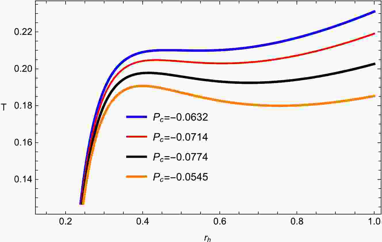
It has a peak as shown in Figs. 1 and 2 and that shifts to right (positive) and increases by increasing $ P_c $ and $ \kappa_{s} $. The temperature becomes the absence of the electric charge $ (q= 0) $. As, we increase the values of $ P_c $ and $ \kappa_{s} $, the the local maximum of the Hawking temperature increases in Figs. 1 and 2. Further, the temperature converges when the horizon radius shrinks to zero for the considered BH manifold. The general form of the first law of BH thermodynamics can be written as [29−32, 46, 47]

Figure 1.  (color online) Plot of temperature T with fixed $ q_{e}=0.28 $; $ q_m=0.08 $; $ d_1=0.004 $; $ f_1=0.313 $; $ \kappa _d =0.02 $; $ \kappa_s =0.8 $ and $ e_{1}=0.4 $.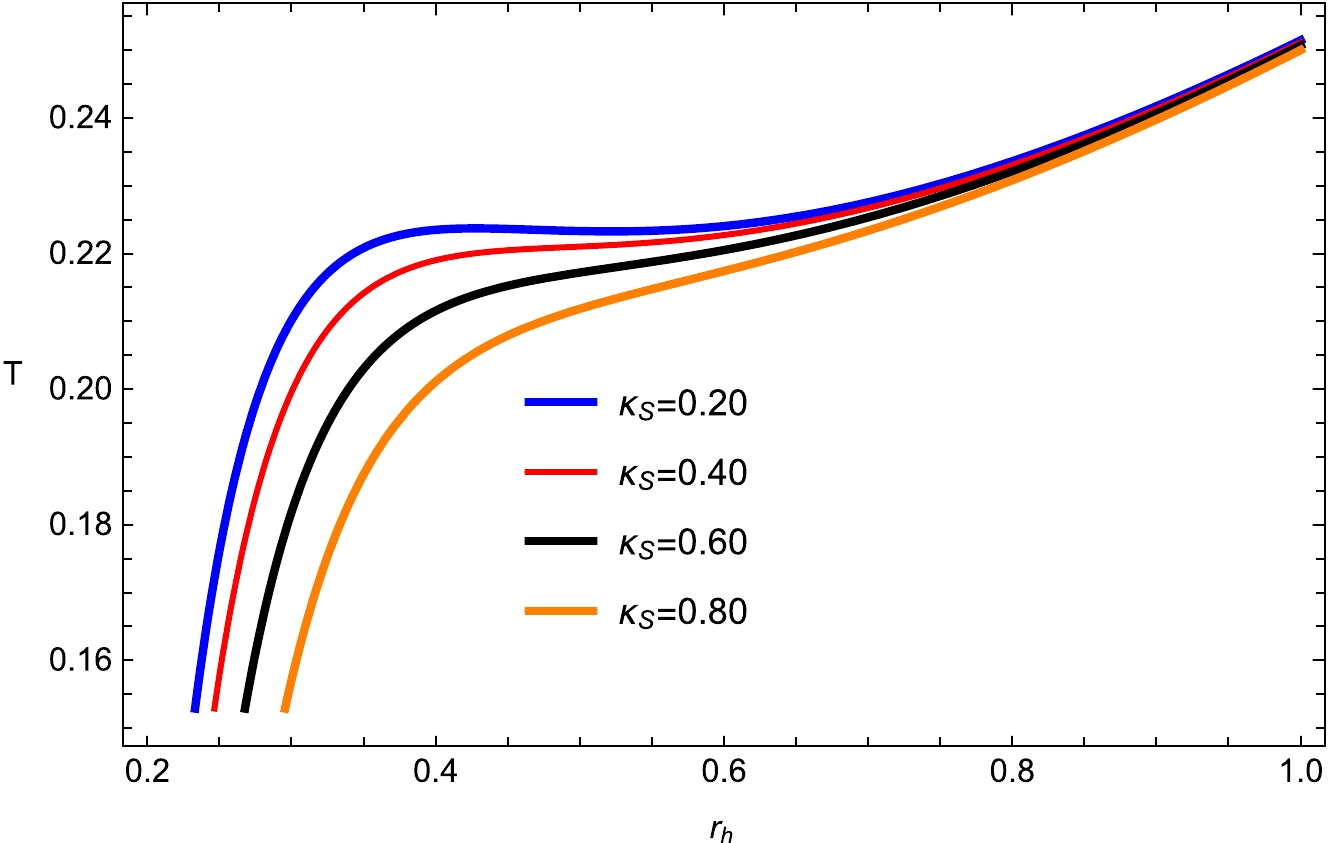

Figure 2.  (color online) Plot of temperature T with fixed $ q_{e }=0.28 $; $ q_m=0.08 $; $ d_1=0.004 $; $ f_1=0.313 $; $ \kappa_d =0.02 $ and $ e_1=0.4 $.

where M, S, V, P, Q, Φ and φ are the mass, entropy, volume, pressure, magnetic charge, and chemical potential of BH, they have been treated as thethermodynamic variables corresponding to the conjugating variables $ \Bbbk_{sh} $, $ \Bbbk_{s} $, $ \Bbbk_{d} $, $ E1 $ and $ d_1 $ respectively. The volume and chemical potential of BH are defined as

respectively. The BH entropy with the help of area is defined as [48−50]

From Eqs. (6) and (7), the equation of state for the BH can easily be expressed as

Red, blue, orange, and black colors indicate the divergence at pressures below the critical pressure. The oscillations of the isotherms at critical temperatures in the $ P - v_h $ diagram are equivalent to the unstable BHs that are presented by negative heat capacity in this section (Figs. 3 and 4). These divergences are the characteristics of the first-order phase transition that occurs between smaller and larger BHs that are stable and have a positive heat capacity. In response to changes in the value of the parameter $ T_c $, there is a corresponding shift in the horizontal axis; an increase in this parameter results in a reduction in the critical radius.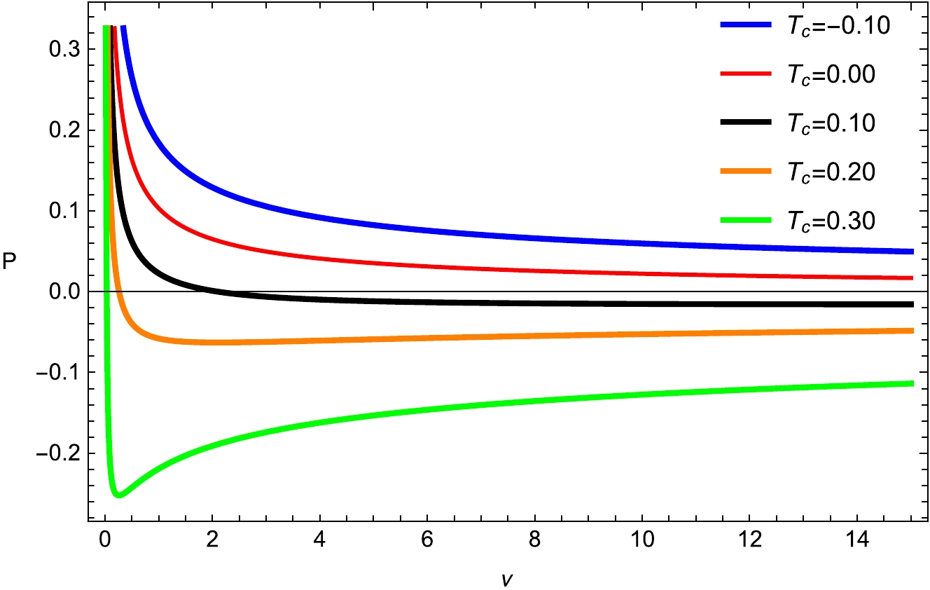

Figure 3.  (color online) Plot of temperature P with fixed $ q_m=0.0002 $; $ d_1=0.004 $; $ f_1=0.003 $; $ \kappa _d =0.01 $; $ \kappa _s =0.03 $ and $ e _1=0.4 $.

Figure 4.  (color online) Plot of temperature P with fixed $ q_m=0.0002 $; $ d_1=0.004 $; $ f_1=0.003 $; $ \kappa _d =0.01 $; $ \kappa _s =0.03 $ and $ e _1=0.4 $.

The thermodynamic variables V, Φ, φ and the conjugating quantities $ \Bbbk_{sh} $, $ \Bbbk_{s} $, $ \Bbbk_{d} $, $ E1 $ and $ d_1 $ are obtained from the first law as

The most important and basic thermodynamic quantity is Gibbs free of BH, it can be utilized to explore small/larger BH phase transition by studying $ G-r_h $ and $ G - T $ diagrams. In addition, Gibbs free energy also helps us to investigate the global stability of BH. It can be evaluated as [ 53, 54]

Using Eqs. (6) and (7) in (13), we get

We observe the graphical behavior of the phase transitions in $ G-r_{h} $ plane as shown in Figs. 5 and 6. It is noted that the Gibbs free energy decreases as the critical radius increases. To calculate the critical thermodynamic properties of BH one can use the following condition, given by [55]

Figure 5.  (color online) Plot of Gibbs free energy G with fixed $ q_m=0.003 $; $ d_1=0.200 $; $ f_1=0.050 $; $ \kappa _d =0.010 $ and $ e _1=0.050 $.

Figure 6.  (color online) Plot of Gibbs free energy G with fixed $ q_m=0.003 $; $ d_1=0.200 $; $ f_1=0.050 $; $ \kappa _d =0.010 $ and $ e _1=0.050 $.

Using Eq.(15), the critical temperature can be expressed as

From Eq. (15), the critical radius of BH, yields as

The critical pressure in terms of other parameters takes the following form

However, we employed numerical analysis because calculating the critical numbers analytically is not a simple operation.

To find more data about a phase transition, we study thermodynamic a quantity such as heat capacity. By applying the standard definition of heat capacity follows as [46, 56]

with little numerical calculations, one can get a dimensionless important relation for the amounts $ P_c $, $ T_c $ and $ v_c $. If provided expression $ (d_1 \kappa_{s}^2-2 f_1 \kappa_{\text{sh}}^2+q_e^2+q_m^2-4 \kappa_d ^2 e_{1})\rightarrow 1.327765310 $, then our solution satisfied the well-known condition as

which is similar results are studied in the context of the Van der Waals equation and in RN-AdS BH . Therefore, the negative heat capacity gives the temperamental (unstable) BH is also related to the critical temperature in $ P-\upsilon_{h} $ plane. By using expressions of volume and entropy of BH is studied in (7) and (10). From Eq. (19), we get

It has been discovered that the critical amounts classify the behavior of thermodynamic quantities close to the critical point. In Figs. 7 and 8, For thermodynamically stable BHs, we separate the two cases in which the heat capacity is positive ($ r _h <r_ c $) and the case in which it is negative ($ r_ h> r_ c $). The second-order phase transition is implied by the instability areas of BHs, where the heat capacity is discontinuous at the critical temperature $ r _h=r _c $ [51, 52]. It is noted that the heat capacity diverges at $ r_h = 0.50 $, when $ T_h $ reaches its maximum value as $ T_h=0.24 $ for $ r_h = 1.00 $, $ q_m=0.08 $, $ d_1=0.004 $, $ f_1=0.313 $, $ \kappa _d =0.02 $ and $ e _1=0.4 $. The critical points in alternate phase space are obtained by utilizing the standard definition, we reduced the thermodynamic variables as

Figure 7.  (color online) Plot of Heat capacity with fixed $ q_m=0.08 $; $ d_1=0.004 $; $ f_1=0.313 $; $ \kappa _d =0.02 $ and $ e _1=0.4 $.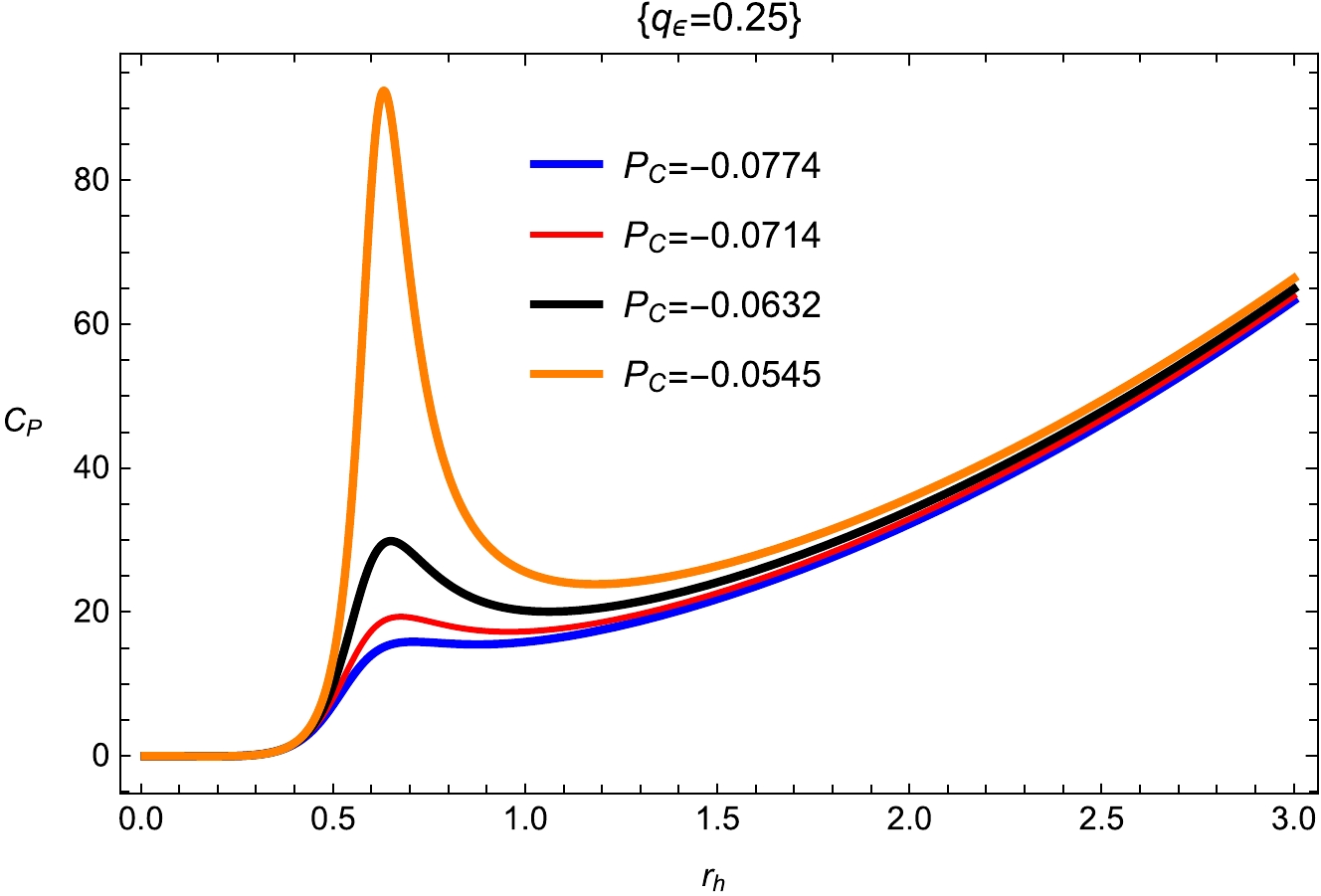

Figure 8.  (color online) Plot of Heat Capacity with fixed $ q_m=0.08 $; $ d_1=0.004 $; $ f_1=0.313 $; $ \kappa _d =0.02 $ and $ e _1=0.4 $.

The reduced variables can be written as

and volume can be obtained as

and pressure follows as

Two adiabatic and two isothermal processes combine to form the Carnot cycle is the hallmark of the most effective heat engine. The single most fundamental and critical feature of the Carnot cycle is that reservoir temperatures as a function of heat engine efficiency

As a reservoir can never be at zero temperature, the efficiency cannot be one since $ T_c $ is cold and $ T_h $ denotes hot reservoirs. Hence, we get

Now, we study the behavior of the heat engine efficiency η as a function of the the pressure P and entropy S matching to the heat cycle provided in Figs. 9 and 10, for the different values of metric-affine gravity parameters. From these figures, we distinguish that the nature of the heat engine efficiency is essentially relying on the metric-affine gravity parameters. In addition, for a given set of input values, the efficiency of the heat engine increases monotonically as the horizon's radius grows. Because of this, larger BHs should expect higher heat-engine efficiency. In other words, they allow for a maximum efficiency curve to be provided for a heat engine by varying only a few fixed parameters (BH works at the highest efficiency). Here, local stability is related to the system, but it can be great to the small changes in the values of thermodynamic parameters. Thus, the term heat capacity gives information on local stability. In [36], it is stated how the cosmological constant Λ can be studied by treating it as a scale parameter.

Figure 9.  (color online) Plot of Efficiency η with fixed $ q_m=0.08 $; $ d_1=0.004 $; $ f_1=0.313 $; $ \kappa _d =0.02 $ and $ e _1=0.4 $.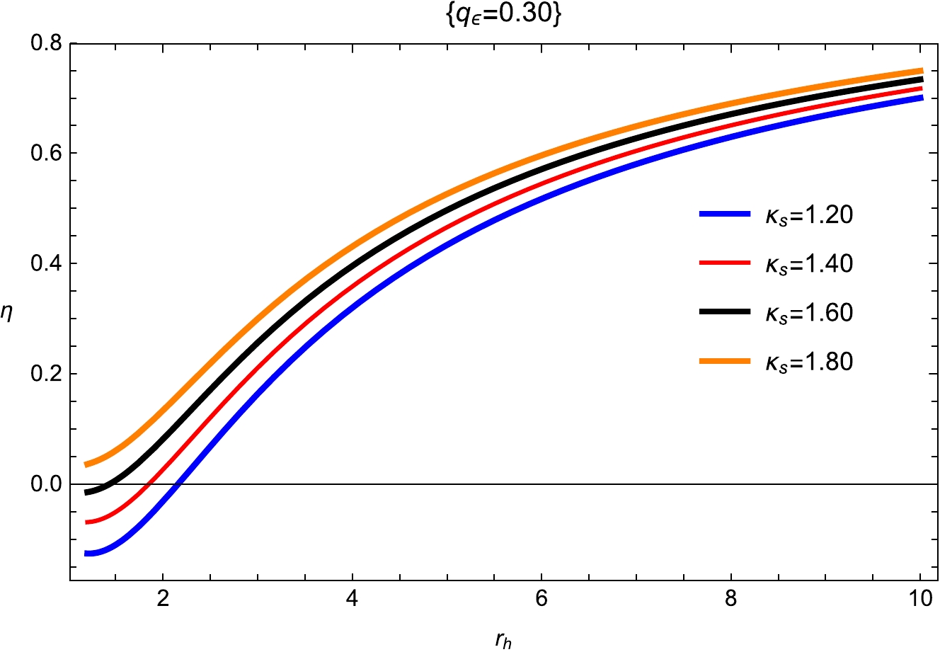

Figure 10.  (color online) Plot of Efficiency η with fixed $ q_m=0.08 $; $ d_1=0.004 $; $ f_1=0.313 $; $ \kappa _d =0.02 $ and $ e _1=0.4 $.

One of the most well-known and classical physical process to explain the change in the temperature of gas from a high-pressure section to reduced pressure through a porous plug is called Joule-Thomson expansion. The main focus is on the gas expansion process, which expresses the cold effect (when the temperature drops) and the heat effect (when the temperature increases), with the enthalpy remaining constant throughout the process. This change depends upon the coefficient of Joule-Thomson as [28, 57]

Using Eqs. (7), (9), (21) and (28) coefficient calculated as

The study of coefficient of Joule-Thomson versus the horizon $ r_h $ is shown in Figs. 11, 12, 13 and 14. We set $ d_1=0.004 $, $ f_1=0.313 $, $ \kappa _{sh} =0.05 $, $ \kappa _d =0.02 $, $ \kappa _s =0.8 $ and $ e _1=0.4 $ in the order. There exist both divergence points and zero points for different variations $ \kappa _d $, $ \kappa _s $, and $ \kappa _{sh} $ respectively. It is clear from a comparison of these figures that the zero point of the Hawking temperature and the divergence point of the coefficient of Joule-Thomson is the same. This point of divergence gives information on the Hawking temperature and corresponds to the most extreme BHs. From Eq. (29) utilizing the well known condition $ \mu_{JT}=0 $, the temperature inversion occurs as

Figure 11.  (color online) Joule-Thomson coefficient $ \mu_{JT} $ Plane with fixed $ d_1=0.03 $; $ f_1=0.01 $; $ \kappa _{d} =0.02 $; $ \kappa _s =0.10 $ and $ e _1=0.04 $.

Figure 12.  (color online) Joule-Thomson coefficient $ \mu_{JT} $ with fixed $ d_1=0.03 $; $ f_1=0.01 $; $ \kappa _{d} =0.02 $; $ \kappa _s =0.10 $ and $ e _1=0.04 $.

Figure 13.  (color online) Joule-Thomson coefficient $ \mu_{JT} $ with fixed $ d_1=0.03 $; $ f_1=0.01 $; $\kappa _{\rm sh} =0.10$; $ \kappa _d =0.02 $ and $ e _1=0.04 $.

Figure 14.  (color online) Joule-Thomson coefficient $ \mu_{JT} $ with fixed $ d_1=0.03 $; $ f_1=0.01 $; $\kappa _{\rm sh} =0.10$; $ \kappa _s =0.10 $ and $ e _1=0.04 $.

Since the Joule-Thomson expansion is an isenthalpic process, it is important to analyze the isenthalpic curves of BHs under metric-affine gravity that is depicted in Figs. 15−18. So, we study isenthalpic curves ($ T_i -P_i $- plane) by assuming different values of BH mass which investigated in Eq. (29) with a larger root of $ r_h $. We show the isenthalpic curves and the inversion curves of BH in metric-affine gravity and this result is consistent [58, 59, 66, 67]. Heating and cooling zones are characterized by the inversion curve, and isenthalpic curves possess positive slopes above the inversion curve. In contrast, the pressure always falls in a Joule-Thomson expansion and the slope changes sign when heating happens below the inversion curve. The heating process appears at higher temperatures, as indicated by the negative slope of the constant mass curves in the Joule-Thomson expansion. When temperatures drop, cooling begins, which is linked to the positive slope of the constant mass curves. From above equation, one can deduced the inversion pressure as

Figure 15.  (color online) Isenthalpic curves $ (T-P) $ Plane with fixed $ d_1=0.004 $; $ f_1=0.313 $; $\kappa _{\rm sh} =0.05$; $ \kappa _d =0.02 $; and $ e _1=0.4 $.

Figure 16.  (color online) Isenthalpic curves $ (T-P) $ Plane with fixed $ d_1=0.004 $; $ f_1=0.313 $; $ \kappa _d =0.02 $; $ \kappa _s =0.8 $ and $ e _1=0.4 $.

Figure 17.  (color online) Isenthalpic curves $ (T-P) $ Plane with fixed $ d_1=0.004 $; $ f_1=0.313 $; $\kappa _{\rm sh} =0.05$; $ \kappa _d =0.02 $; $ \kappa _s =0.8 $ and $ e _1=0.4 $.

Figure 18.  (color online) Isenthalpic curves $ {T-P} $ Plane with fixed $ d_1=0.004 $; $ f_1=0.313 $; $\kappa _{\rm sh} =0.05$; $ \kappa _d =0.02 $; $ \kappa _s =0.8 $ and $ e _1=0.4 $.

The inversion curves for different values $ d_1=0.004 $, $ f_1=0.313 $, $ \kappa _{sh} =0.05 $, $ \kappa _d =0.02 $ are shown in Figs. 19, 20, 21 and 22. The inversion temperature increases with variations of important parameters m, $ q_e $, $ \kappa _{sh} $ and $ \kappa _s $ respectively. We can go back to the case of BH in metric-affine gravity. Compared with the van der Waals fluids, we see from Figs. 19−22 that the inversion curve is not closed. From the above results, in $ Ti-Pi $-plan at low pressure, the inversion temperature $ T_i $ decreases with the increase of charge $ q_e $ and mass m, which shows the opposite behavior for higher pressure. It is also clear that, unlike the case with van der Waals fluids, the inversion temperature continues to rise monotonically with increasing inversion pressure, and hence inversion curves are not closed [66, 67].

Figure 19.  (color online) Inversion curves $ (Ti-Pi) $ with fixed $ d_1=0.004 $; $ f_1=0.313 $; $\kappa _{\rm sh} =0.05$; $ \kappa _d =0.02 $; $ \kappa _s =0.8 $ and $ e _1=0.4 $.

Figure 20.  (color online) Inversion curves $ (Ti-Pi) $ with fixed $ d_1=0.004 $; $ f_1=0.313 $; $\kappa _{\rm sh} =0.05$; $ \kappa _d =0.02 $; $ \kappa _s =0.8 $ and $ e _1=0.4 $.

Figure 21.  (color online) Inversion curves $ (Ti-Pi) $ Plane with fixed $ d_1=0.004 $; $ f_1=0.313 $; $ \kappa _d =0.02 $; $ \kappa _s =0.8 $ and $ e _1=0.4 $.

Figure 22.  (color online) Inversion curves $ (Ti-Pi) $ Plane with fixed $ d_1=0.004 $; $ f_1=0.313 $; $\kappa _{\rm sh} =0.05$; $ \kappa _d =0.02 $ and $ e _1=0.4 $.

In this paper, we have considered BH in metric-affine gravity and studied thermodynamics in presence of Bekinstien entropy, and examined the standard thermodynamics relations. In detail, we have thoroughly investigated thermodynamics to analytically obtain thermodynamical properties like the Hawking temperature, entropy, specific heat, and free energy associated with BH in metric-affine gravity with a focus on the stability of the system. The heat capacity blows at $ r_c $, which is a double horizon, and local maxima of the Hawking temperature also occur at $ r_c $. It is shown that the heat capacity is positive for $ r_h < r_c $ providing the stability of small BHs close-up to perturbations in the region, and at critical radius phase transition exists. While the BH is unstable for $ r_h > r_c $ with negative heat capacity. The global analysis of the stability of BH is also discussed by calculating free energy $ G_h $. For negative free energy $ G_h < 0 $ and positive heat capacity $ C_p > 0 $, it is noted that smaller BHs are globally stable, and also these results are used in Refs. [14−19]. We calculated the inverse temperature, inverse pressure and mass parameter, which investigated the Joule-Thomson process of the system. The negative cosmological constant in metric-affine gravity is investigated to phase transitions of BHs. Above the inversion curves, we examined the cooling region, while below the inversion curve it leads to the heating one. The corresponding results can be summarized as: both the inversion temperature and pressure are become greater with the increasing of BH in metric-affine gravity while they are decreasing with the charge $ q_e $. The physical consequences was analogous with the holography, where BHs would being a system as well as dual to conformal field theories. The BH in metric-affine gravity is studied and identical to the thermodynamics of usual systems and their thermodynamical analysis become more complete. Our results show a characteristic of Joule-Thomson coefficient is independent of the shear, spin and dilation charges indicating that the Joule-Thomson expansion we consider here is universal. In particular, we find a novel isenthalpic curves in which the inversion temperature of the Joule-Thomson expansion, rather than the extreme one reported by previous work separates the analogues to heating-cooling phase [60−62]. Therefore, our inversion curves separates the allowable along with forbidden regions for the Joule-Thomson effect to be observed, where the Joule-Thomson coefficient is the essential quantity to discriminate between the cooling and heating regimes of the system. It is worth noting that when amplify a thermal system with a temperature so that pressure always decreases yielding a negative sign to $ \partial P $.

Our analysis of inversion curves in the plane revealed that the influence of the parameters a BH may be more evident in space-time. We analyzed the BH in metric-affine gravity characteristics on the inversion curve; these included the the shear, spin and dilation charges. In these figures, we observed that the inversion curves be compatible with the extreme point of a specific isenthalpic curves, and the cooling as well as heating regions are identified. In other words, the boundary between the heating-cooling regions of the BH in metric-affine gravity influence on the inversion curves. We also discovered that both the maximum expansion points of cooling-heating regimes like [63−65]. For the BH heat engine, we investigated the analytical expression for the efficiency in terms of horizon radius, pressures and temperatures in various limits. We have also studied the Joule-Thomson expansion, isenthalpic curves and inversion curves of the considered BH in metric affine gravity as given below:

● We have examined the Joule-Thomson expansion for BH in metric-affine gravity, where the cosmological constant is taken as a pressure. We mainly focused on BH mass is considered enthalpy, it is the mass that does not change during the expansion. The Joule-Thomson coefficient $ \mu_{JT} $ in terms of horizon $ r_h $ is shown in Figs. 11−14. There exist both divergence points and zero points with $ d_1=0.004 $, $ f_1=0.313 $, $\kappa _{\rm sh} =0.05$, $ \kappa _d =0.02 $, $ \kappa _s =0.8 $ and $ e _1=0.4 $. The zero point of the Hawking temperature, which is related to the most distant BHs, agrees with the divergence point of the Joule-Thomson coefficient, which is depicted in a consistent manner [66, 67].

● We also presented the isenthalpic curves such results are presented in higher dimensions as demonstrated in Figs. 15−18. It is very interesting to explain that the positive slopes of the inversion curve are found as mentioned in the literature [28, 57]. This indicates that with the expansion of a metric-affine universe, BH always cools above the inversion curve.

● To determine the temperature gradients between the cooling and heating zones for various values of $ d_1 $, $ f_1 $, $ \kappa _{sh} $ and $ \kappa _d $, we have analyzed the inversion curve (Figs. 19−22).

It is concluded that the considered BH in metric affine gravity meets the results in the literature and also this work is beneficial for future research.

The authors declare that they have no known competing financial interests or personal relationships that could have appeared to influence the work reported in this paper.

This manuscript has no associated data, or the data will not be deposited. (There is no observational data related to this article. The necessary calculations and graphic discussion can be made available on request.)