Pair production of the isosinglet vector-like leptons at the ${\boldsymbol e^{\bf +}\boldsymbol e^{\bf -}}$ colliders

Vector-like leptons (VLLs) constitute a particularly well-motivated extension of the Standard Model (SM), emerging naturally in diverse beyond-Standard-Model (BSM) scenarios that address several theoretical challenges. These include resolving the hierarchy problem through modified Higgs sector dynamics [1], providing viable dark matter candidates [2−5], stabilizing the electroweak vacuum [6, 7], and explaining precision anomalies such as the muon's anomalous magnetic moment [8−12] and observed discrepancies in the W boson mass [13, 14]. The theoretical appeal of VLLs is further enhanced by their natural incorporation into broader frameworks, including extra-dimensional models [15, 16], supersymmetric extensions [17−21], and various other SM extensions [22−25]. Unlike the chiral SM fermions, VLLs possess left- and right-handed components with identical gauge transformations, enabling gauge-invariant mass terms independent of the Higgs mechanism. This distinctive property renders them less constrained than additional chiral fermions by both electroweak precision tests [26, 27] and Higgs boson measurements [28−30], while offering rich phenomenology (for example see [31−53]).

Current experimental searches by ATLAS and CMS primarily investigate VLL pair production with subsequent decays to Standard Model bosons and tau leptons [54−59]. For doublet VLLs, these searches exclude masses in the range 130-900 GeV (ATLAS, 139 fb⁻¹ at 13 TeV) [55] and up to 1045 GeV (CMS, 138 fb⁻¹ at 13 TeV) [57], while singlet VLLs remain less constrained with current limits below 150 GeV. A specialized CMS analysis using 77.4 fb⁻¹ of 13 TeV LHC data has further excluded flavor-specific $ S U(2)_{L} $ singlet VLLs up to approximately 300 GeV and doublet VLLs to about 800 GeV [60].

As shown in Ref. [61], weak-isosinglet VLLs present significant detection challenges at hadron colliders due to overwhelming QCD backgrounds. Future high-energy $ e^+e^- $ colliders, such as the International Linear Collider (ILC) [62, 63] and Compact Linear Collider (CLIC) [64, 65], provide a cleaner environment for VLL searches [66−71]. In this work, we investigate a weak isosinglet VLL ($ \tau' $) that mixes minimally with the SM tau lepton. We analyze $ \tau^{\prime+}\tau^{\prime-} $ pair production via $ e^+e^- \to \tau^{\prime+}\tau^{\prime-} $ at center-of-mass (c.m.) energies of $ \sqrt{s} = 1 $ TeV (ILC) and 1.5 TeV (CLIC), focusing on the dominant decay channels $ \tau'\to W\nu_\tau $, $ Z\tau $, and $ h\tau $. Through detailed signal-background analyses, we derive $ 2\sigma $ exclusion sensitivity and $ 5\sigma $ discovery reach as functions of integrated luminosity. Our results demonstrate that future $ e^+e^- $ colliders can probe singlet VLL masses substantially beyond current LHC constrains, extending nearly up to the kinematic threshold.

This paper is organized as follows: In Section II, we present the theoretical framework of the singlet VLL model, including its couplings to Standard Model particles. We derive the pair production cross sections for VLLs at future high-energy $ e^+e^- $ colliders, with particular emphasis on polarization and initial-state radiation effects. In section III, we perform a detailed collider analysis of the relevant signals and backgrounds for two type of final states. Finally, we give a summary in Sec. IV.

The singlet VLL model introduces a pair of charged $ \tau'^{\pm} $ fermions that transform under the SM gauge group $ S U(3)_C \times S U(2)_L \times U(1)_Y $ as two-component fermions:

The relevant mass terms and mixing with SM leptons are described by the Lagrangian [41]:

where H denotes the SM Higgs complex doublet scalar field, $ L = (\tau, \nu_\tau) $ represents the third-generation lepton doublet in the gauge basis, $ y_\tau $ is the SM tau Yukawa coupling, and $ \epsilon $ parameterizes the small mixing between $ \tau' $ and SM leptons.

In the gauge eigenbasis $ (\tau, \tau') $, the mass matrix takes the form:

where $ v \approx 174 $ GeV is the Higgs vacuum expectation value and M is the large mass parameter. The diagonalization of the mass matrix reveals the physical mass eigenvalues:

At leading order in the $ \epsilon $ expansion, the mass eigenstates correspond to: a SM-like τ lepton with mass $ m_\tau = y_\tau v [1 + \mathcal{O}(\epsilon^2)] $, and a predominantly gauge-singlet $ \tau' $ state with mass $ m_{\tau'} = M [1 + \mathcal{O}(\epsilon^2)] $, where the $ \mathcal{O}(\epsilon^2) $ corrections represent the small mixing-induced mass shifts.

Current experimental constraints, particularly from $ Z \to \tau^+\tau^- $ decays and leptonic tau decays [69], require the mixing angle $ \theta_L $ to satisfy: $ \sin \theta_L=\dfrac{\epsilon v}{m_{\tau'}}\lesssim 0.029 $. Throughout our analysis, we assume $ \epsilon $ is sufficiently small to treat mixing effects perturbatively, while remaining large enough ($ \epsilon \gtrsim 2\times10^{-7} $) to ensure prompt $ \tau' $ decays within detector volumes [41]. For smaller mixing values leading to displaced decays, dedicated searches for long-lived charged particles would become relevant [50, 72].

The partial decay widths of $ \tau' $ to SM final states are given by:

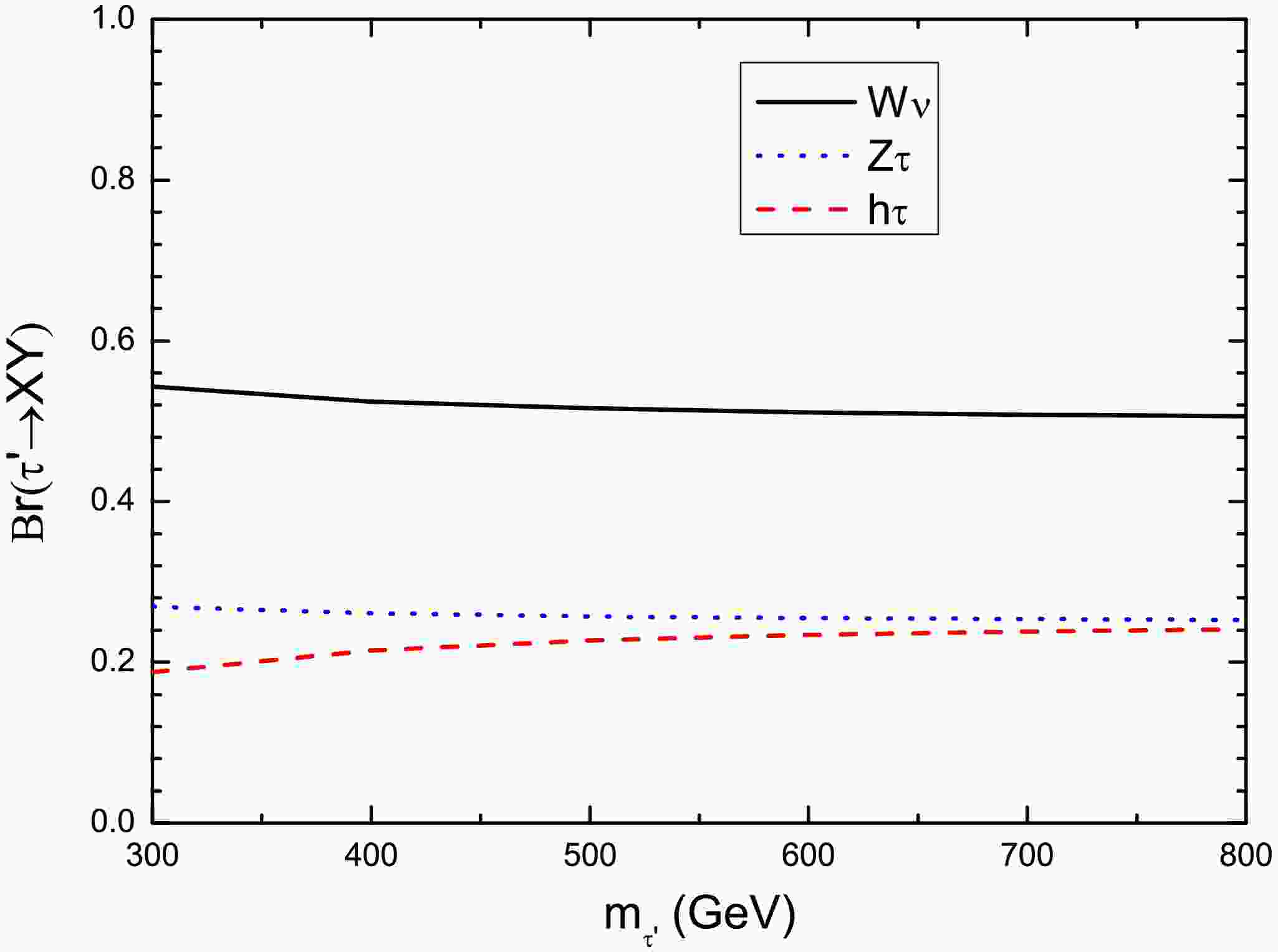
where $ r_X = m_X^2/m_{\tau'}^2 $ for $ X = W, Z, h $. In the heavy $ \tau' $ limit ($ m_{\tau'}\gg m_{W,Z,h}) $, the branching ratios asymptotically approach the characteristic pattern:

as demonstrated in Figure 1, which shows the mass dependence of these branching fractions.

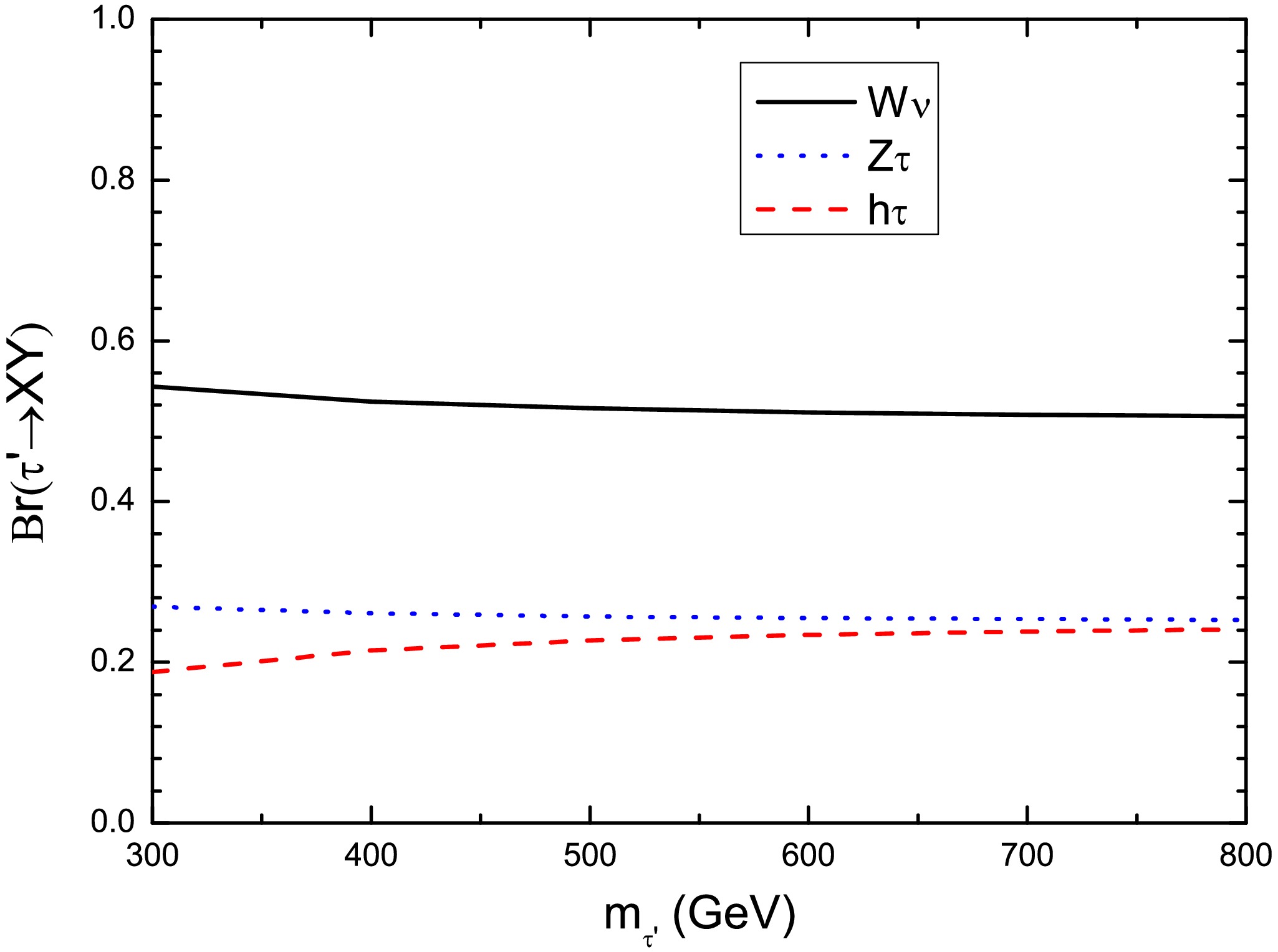
Figure 1.  (color online) Branching ratios of weak isosinglet vector-like leptons $ \tau' $ as functions of $ m_{\tau'} $.

The pair production of VLLs is primarily mediated through their flavor-diagonal couplings to electroweak gauge bosons. In the two-component fermion formalism (with metric signature -+++), the leading-order interaction Lagrangian for the singlet VLL model, retaining terms up to $ \mathcal{O}(\epsilon) $, reads:

where e denotes the electromagnetic coupling, g is the $ SU(2)_L $ gauge coupling, $ \theta_{W} $ is the Weinberg angle, and $ s_W \equiv \sin\theta_W $, $ c_W \equiv \cos\theta_W $ are the weak mixing angle with $ e = g s_W $.

For polarized $ e^+e^- $ collisions with beam polarizations $ P_{e^-} $ and $ P_{e^+} $, the partonic cross-section takes the form:

with the chiral amplitude coefficients:

where $ \hat{s} $ represents the effective c.m. energy accounting for beam energy spread ($ \hat{s} < s $). The production cross-section is maximized when $ P_{e^-} $ is positive and $ P_{e^+} $ is negative, owing to the hierarchy $ |a_L| < |a_R| $ for $ \sqrt{\hat s} > 93 $ GeV.

Our analysis considers three collider scenarios:

● ILC: $ \sqrt{s} = 1 $ TeV with $ (P_{e^+}, P_{e^-}) = (-0.2, 0.8) $ (20% left-handed positrons, 80% right-handed electrons),

● CLIC: $ \sqrt{s} = 1.5 $ and 3 TeV with $ (P_{e^+}, P_{e^-}) = (0, 0.8) $ (unpolarized positrons, 80% right-handed electrons),

as motivated by technical feasibility studies [62]. Polarization values follow the convention where $ P = +1 $ ($ -1 $) denotes fully right-handed (left-handed) particles. Certainly, these choices would maximize the cross-sections for the signal at ILC and CLIC designs, respectively.

In our collider analysis, we adopt the leading-order approximation $ m_{\tau^{\prime}} \approx M $, which remains valid because the physical mass correction $ \delta m_{\tau^{\prime}} = \mathcal{O}(\epsilon^2) $ becomes negligible when $ \epsilon \ll 1 $, as confirmed by recent benchmark studies [52]. Importantly, both the $ \tau^{\prime} $ branching ratios (Eqs. (6)-(8)) and production cross section (Eq. (11)) show no dependence on $ \epsilon $. This allows us to focus our investigation on discovery potential through systematic $ m_{\tau^{\prime\pm}} $ scans, providing a completely model-independent approach to studying $ \tau^{\prime} $ phenomenology at future $ e^+e^- $ colliders that requires no assumptions about the $ \epsilon $ parameter space.

Figure 2 presents the $ \tau^{\prime+}\tau^{\prime-} $ pair production cross sections $ \sigma(e^+e^-\rightarrow \tau^{\prime+}\tau^{\prime-}) $ as a function of $ m_{\tau^\prime} $, including both initial state radiation (ISR) and beam polarization effects. Note that these effects are calculated at leading order (LO) by using $ \mathtt{MADGRAPH5_AMC@NLO} $ [73] where some commands in the run_card file are given in Appendix A. One can see that, for $ \sqrt{s}=1 $ TeV ($ m_{\tau^\prime}\in[200,490] $ GeV), ISR modifies the cross sections by factors ranging from 1.1 to 0.66, while for $ \sqrt{s}=1.5 $ TeV ($ m_{\tau^\prime}\in[500,740] $ GeV) and $ \sqrt{s}=3 $ TeV ($ m_{\tau^\prime}\in[800,1490] $ GeV), the corresponding ISR correction factors vary between 0.91–0.61 and 0.64–1.57, respectively, demonstrating the significant impact of ISR that must be accounted for in precision calculations at future $ e^+e^- $ colliders. This is because the ISR effect modifies the effective c.m. energy $ \sqrt{s'} $, leading to a slight enhancement of the cross-section in the low-mass region due to resonant enhancement and soft-photon dominance, while strongly suppressing the cross-section in the high-mass region through phase-space suppression and threshold effects. On the other hand, the implementation of beam polarization yields particularly enhanced production rates, with cross sections reaching approximately 94 fb (450 GeV at 1 TeV), 27.8 fb (700 GeV at 1.5 TeV), and 5.9 fb (1400 GeV at 3 TeV), underscoring the substantial benefits achievable through polarized beams in high-mass regimes.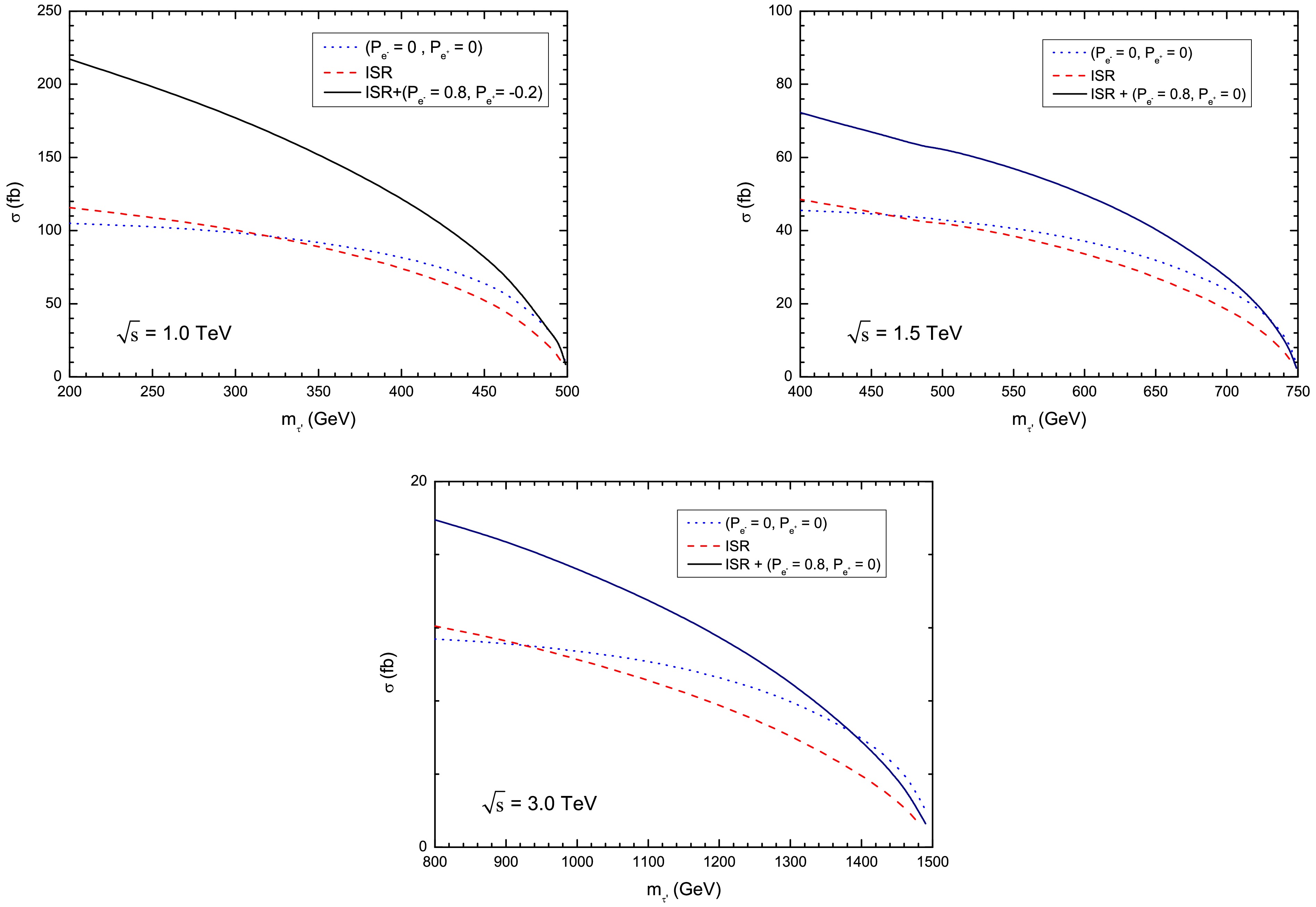

Figure 2.  (color online) Production cross-sections for $ e^+e^-\to \tau^{\prime +}\tau^{\prime -} $ including ISR and polarization effects. The beam polarization configurations are: $ (P_{e^+}, P_{e^-}) = (-0.2, 0.8) $ for $ \sqrt{s} = 1.0 $ TeV, $ (P_{e^+}, P_{e^-}) = (0, 0.8) $ for $ \sqrt{s} = 1.5 $ and 3 TeV, respectively.

We analyze the discovery potential through Monte Carlo simulations of signal and background events, investigating the sensitivity to single VLLs via the decay channels $ \tau'^{\pm}\to W^{\pm}\nu_{\tau} $, $ \tau'^{\pm}\to Z\tau^{\pm} $, and $ \tau'^{\pm}\to h\tau^{\pm} $. Considering the subsequent decays $ W^{\pm}\to jj $, $ Z\to \ell^{+}\ell^{-} $, $ W^{\pm}\to \ell^{\pm}\nu_{\ell} $, and $ h\to b\bar{b} $, we focus on two characteristic final states:

● Case 1: $ e^{+}e^{-}\to \tau'^{+}\tau'^{-}\to Z\tau^{\pm}W^{\mp}\nu_{\tau}\to 2\ell+2j + 1\tau + \not {E}_{T} $,

● Case 2: $ e^{+}e^{-}\to \tau'^{+}\tau'^{-}\to h W^\pm \tau^\mp\nu_{\tau}\to 1\ell+2b +1\tau + \not {E}_{T} $,

where $ \ell = e,\mu $, j refers to a non-b jet, and $ \not{E}_{T} $ denotes the missing energy. The corresponding Feynman diagrams for the production and decay chains are shown in Fig. 3.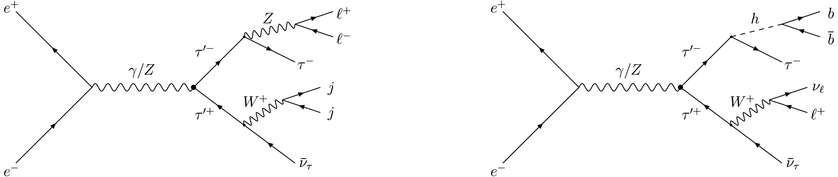

Figure 3.  Representative Feynman diagrams for case 1 and case 2.

We generate signal and SM background events at leading order using $ \mathtt{MADGRAPH5} $ [73], with subsequent showering and fragmentation handled by $ \mathtt{PYTHIA} $ 8.20 [74]. Detector effects are simulated with $ \mathtt{DELPHES} $ 3.4.2 [75], with the ILD detector configuration for ILC studies and the CLIC detector configuration ($ \mathrm{delphes{\_}card{\_}CLICdet{\_}Stage3{\_}fcal.tcl}$) [76] for CLIC analyses. Jet clustering is performed with the Valencia Linear Collider (VLC) algorithm [77, 78] with parameters: $ R = 0.5 $, $ \beta = 1 $, $ \gamma = 1 $ (see [78] for details), and the b-tagging efficiency and misidentification rates are taken as the medium working points (WP) with a b-tagging efficiency of 70%. Finally, event analysis is performed with $ \mathtt{MADANALYSIS5} $ [79].

The dominant SM backgrounds include: $ ZW^{\pm}\tau^{\mp}\nu_{\tau} $ from $ ZW^{+}W^{-} $ production (including t-channel diagrams and off-shell contributions) for Case 1, and $ hW^{\pm}\tau^{\mp}\nu_{\tau} $ production for Case 2. Additional backgrounds from $ t\bar{t}Z $ and $ t\bar{t} $ are considered for both cases, while other processes like $ Zh $, $ Zhh $, $ ZZh $, and $ t\bar{t}h $ are neglected due to their negligible cross sections after selection cuts. We list their production cross sections with the ISR and polarization effects at $ e^+e^- $ colliders in Table 1. The values in parentheses show the cross-section ratio $ \sigma_{\text{pol}}/\sigma_{\text{unpol}} $, characterizing the polarization effect magnitude. Our results demonstrate that the selected polarization configuration effectively suppresses SM background cross-sections.

Process	Cross section (fb)
	$ \sqrt{s} = 1.0 $ TeV	$ \sqrt{s} = 1.5 $ TeV	$ \sqrt{s} = 3 $ TeV
$ e^{+}e^{-}\to ZW^{\pm}\tau^{\mp}\nu_{\tau} $	2.06 (0.18)	2.05 (0.21)	1.22 (0.21)
$ e^{+}e^{-}\to t\bar{t}Z $	2.65 (0.59)	1.95 (0.54)	1.0 (0.53)
$ e^{+}e^{-}\to hW^{\pm}\tau^{\mp}\nu_{\tau} $	0.19 (0.23)	0.14 (0.26)	0.062 (0.27)
$ e^{+}e^{-}\to t\bar{t} $	144 (0.78)	62.5 (0.70)	28.7 (0.70)

Table 1.  SM background cross sections with ISR and beam polarization effects. The beam polarization configurations are: $ (P_{e^+}, P_{e^-}) = (-0.2, 0.8) $ for $ \sqrt{s} = 1.0 $ TeV, $ (P_{e^+}, P_{e^-}) = (0, 0.8) $ for $ \sqrt{s} = 1.5 $ and 3 TeV, respectively. The values in parentheses are the cross-section ratio $ \sigma_{\text{pol}}/\sigma_{\text{unpol}} $.

Object identification employs the following basic criteria:

where $ \Delta R = \sqrt{\Delta\phi^{2} + \Delta\eta^{2}} $ is the particle separation in the rapidity (η)-azimuth (ϕ) plane and x, y indicate different final particles ($ \ell $, j).

For the signal $ 2\ell+2j +1\tau + \not E_{T} $, the dominant SM backgrounds come from the SM processes $ e^{+}e^{-}\to ZW^{\pm}\tau^{\mp}\nu_{\tau} $ and $ e^{+}e^{-}\to t\bar{t}Z $. For the signal, the leptons $ \ell_{1} $ and $ \ell_{2} $ are two opposite-sign same-flavor leptons that are assumed to be the product of the Z boson decay, and at least two jets are assumed to be the product of the W decay. Meanwhile, for the decay channels $ \tau'^{\pm}\to W^{\pm}\nu_{\tau} $ and $ \tau'^{\pm}\to Z\tau^{\pm} $, one can reconstruct the mass peaks by using the transverse mass ¹ $ M_{T}(j_{1}j_{2}) $, and the invariant mass $ M_{\ell_{1}\ell_{2}\tau} $. According to the characteristics of the signal and backgrounds, in Fig. 4, we plot differential distributions for signals (with $ m_{\tau^\prime}=300 $, 400,450 GeV for $ \sqrt{s}=1.0 $ TeV, and $ m_{\tau^\prime}=500 $, 600,700 GeV for $ \sqrt{s}=1.5 $ TeV) and relevant SM backgrounds, including the invariant mass distribution for the Z boson ($ M_{\ell_{1}\ell_{2}} $), W boson ($ M_{j_{1}j_{2}} $), the invariant mass distribution for the $ \tau' $ ($ M_{\ell_{1}\ell_{2}\tau} $), and the transverse mass distribution for the $ M_{T}(j_{1}j_{2}) $ system. Based on these kinematic distributions, we can impose the following set of cuts: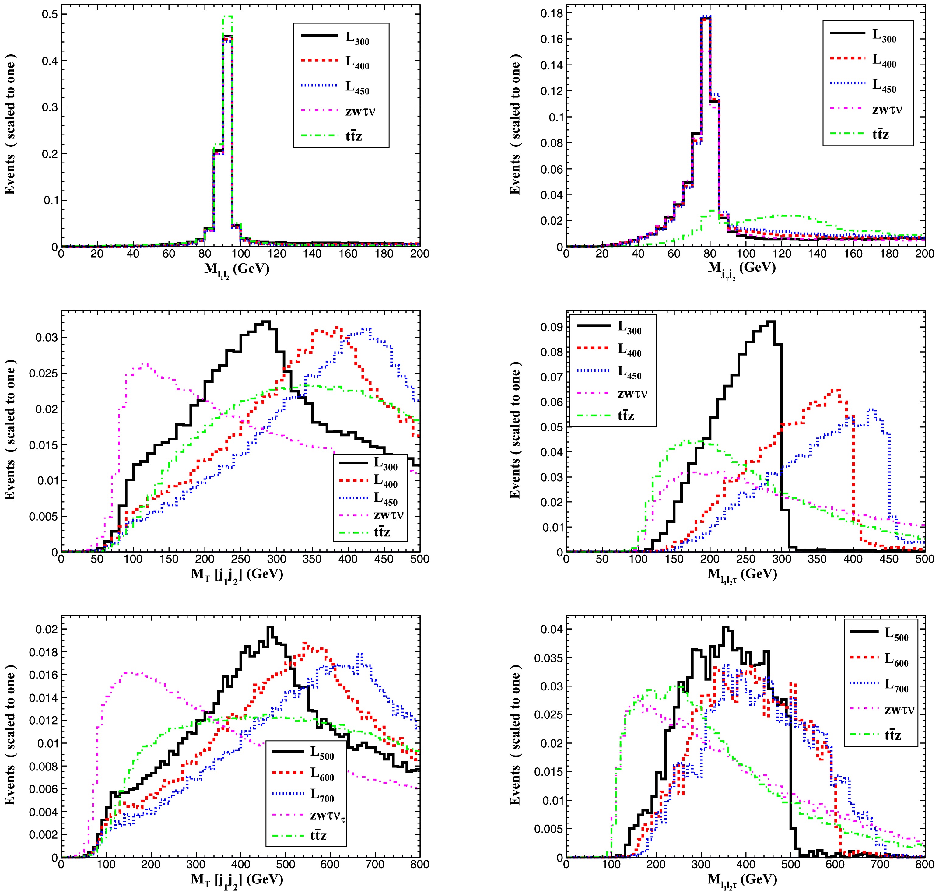

Figure 4.  (color online) Normalized distributions for the signals and relevant SM backgrounds for Case 1.

Cut-1: Object multiplicity:

Exactly two isolated leptons ($ N(\ell)=2 $, $ \ell = e,\mu $)

At least two jets ($ N(j)\geq 2 $)

One τ-tagged jet ($ N(\tau)=1 $)

Cut-2: Invariant mass requirements:

Z mass window: $ |M_{\ell_1\ell_2}-m_Z| < 10\; \text{GeV} $

W mass window: $ 55 < M_{j_1j_2} < 105\; \text{GeV} $

$ \tau' $ candidate: $ M_{\ell_1\ell_2\tau} > 180 $ (300) GeV at $ \sqrt{s}=1.0 $ (1.5) TeV

Cut-3: Transverse mass cuts:

$ M_T(j_1j_2) > 180 $ (300) GeV at $ \sqrt{s}=1.0 $ (1.5) TeV

We report the measured cross sections for signal processes at three benchmark mass points and their corresponding SM backgrounds following the application of sequential selection cuts, as detailed in Tables 2 ($ \sqrt{s}=1.0 $ TeV) and 3 ($ \sqrt{s}=1.5 $ TeV). Note that the cross sections for signal and SM backgrounds are calculated by $ \sigma_{\text{after cut}} = \sigma_0 \times \epsilon_{\text{cut}} $, where $ \sigma_0 $ is the initial cross-section and $ \epsilon_{\text{cut}} $ the cumulative efficiency. Thus the efficiency of each cut can be determined by the ratio of the two adjacent cross-sections. The values in parentheses represent the efficiency after the corresponding cut is applied.

Cuts	Signals				Backgrounds
	300 GeV	400 GeV	450 GeV		$ ZW^{\pm}\tau^{\mp}\nu_{\tau} $	$ t\bar{t}Z $
Basic	2.1	1.46	1.01		0.087	0.023
Cut-1	0.23 (11%)	0.17 (11%)	0.12 (12%)		0.0064 (7%)	0.0027 (11%)
Cut-2	0.19 (8.2%)	0.16 (9.7%)	0.114 (10%)		0.0049 (4.9%)	0.0018 (1.9%)
Cut-3	0.149 (6.9%)	0.134 (8.9%)	0.10 (9.6%)		0.003 (3.3%)	0.0003 (1.45%)

Table 2.  Cut flow of the cross sections (in fb) for signals and backgrounds in Case 1 at $ \sqrt{s}=1.0 $ TeV. The values in parentheses represent the efficiency after the corresponding cut is applied.

Cuts	Signals				Backgrounds
	500 GeV	600 GeV	700 GeV		$ ZW^{\pm}\tau^{\mp}\nu_{\tau} $	$ t\bar{t}Z $
Basic	0.66	0.51	0.28		0.084	0.016
Cut-1	0.058 (8.4%)	0.047 (8.7%)	0.026 (8.8%)		0.0048 (5.2%)	0.0022 (12%)
Cut-2	0.052 (7.1%)	0.043 (7.4%)	0.024 (7.7%)		0.0038 (3.8%)	0.0016 (1.5%)
Cut-3	0.034 (4.9%)	0.031 (5.7%)	0.019 (6.4%)		0.0014 (1.5%)	0.0001 (0.6%)

Table 3.  Cut flow of the cross sections (in fb) for the signals with three typical VLL masses and SM backgrounds for case 1 with $ \sqrt{s}=1.5 $ TeV. The values in parentheses represent the efficiency after the corresponding cut is applied.

For the $ \sqrt{s}=3.0 $ TeV case, we observe similar distributions for both signal and background processes as in the 1.5 TeV analysis, and therefore apply identical selection criteria while omitting the detailed cut flow table for brevity. Our cut flow analysis achieves exceptional background suppression, reducing SM contributions to $ \mathcal{O}(10^{-3}) $ fb while preserving significant signal efficiency. After all selection cuts, the total SM background cross sections are measured to be: $ 3.3\times 10^{-3} $ fb at $ \sqrt{s}=1 $ TeV, $ 1.5\times 10^{-3} $ fb at $ \sqrt{s}=1.5 $ TeV, and $ 0.9\times 10^{-3} $ fb at $ \sqrt{s}=3 $ TeV, respectively.

The signal events are characterized by: exactly one isolated lepton (e or μ), one τ-tagged jet, and at least two b-tagged jets, the dominant SM backgrounds originate from:

● $ e^{+}e^{-}\to hW^{\pm}\tau^{\mp}\nu_{\tau} $ with $ h\to b\bar{b} $ and $ W\to \ell\nu $,

● $ e^{+}e^{-}\to t\bar{t} $ with $ t\to W^{+}b $, where W decays via $ W\to \ell\nu $ or $ W\to \tau \nu_{\tau} $.

To optimize background suppression, we analyzed the normalized distributions of: the invariant mass $ M_{b_{1}b_{2}\tau} $ and the transverse mass $ M_{T}(\ell) $ for signal benchmarks ($ m_{\tau^\prime} = 300 $, 400,450 GeV at $ \sqrt{s} = 1.0 $ TeV; $ m_{\tau^\prime} = 500 $, 600,700 GeV at $ \sqrt{s} = 1.5 $ TeV) and SM backgrounds, as shown in Fig. 5. Based on these kinematic studies, we implement the following selection criteria: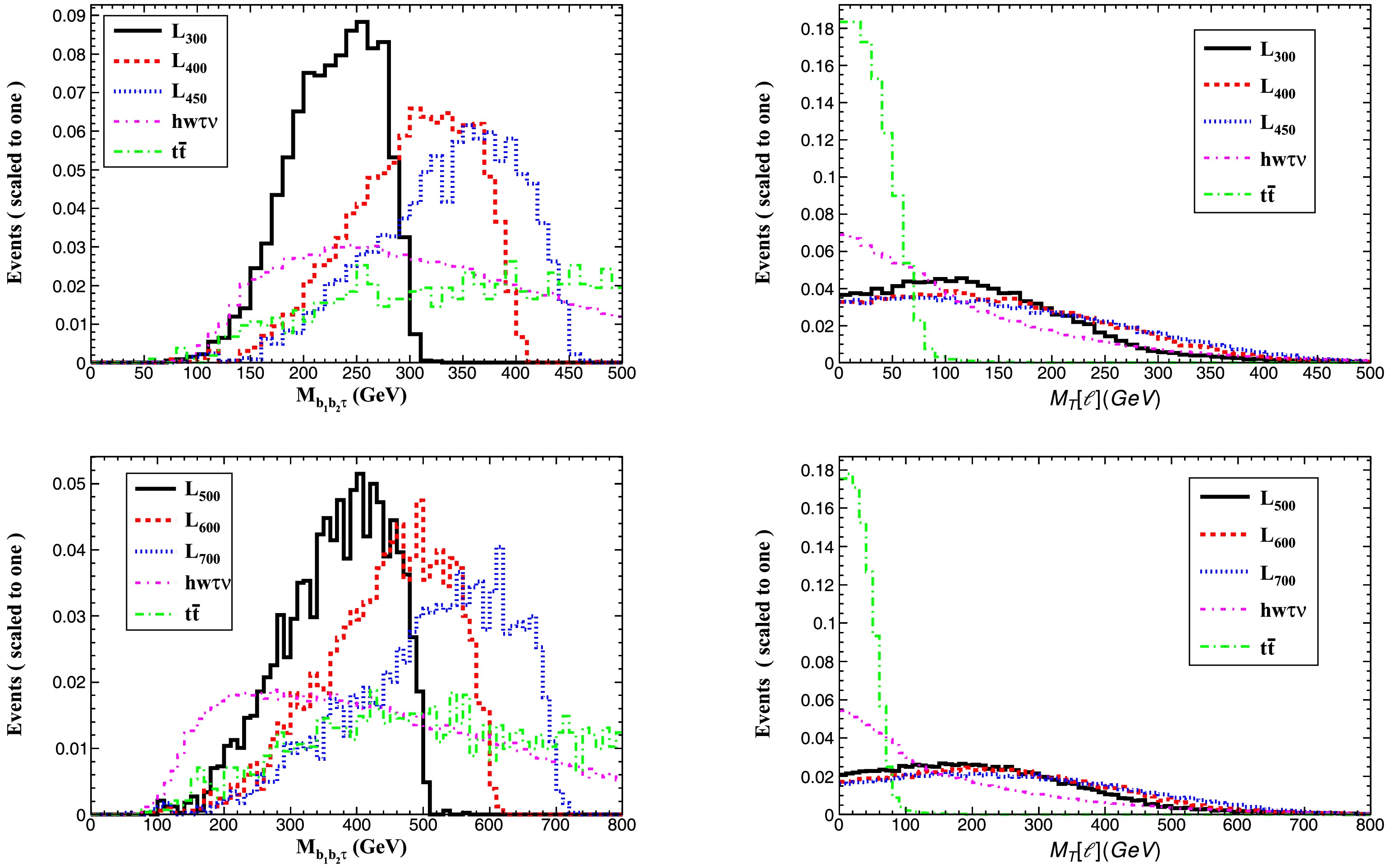

Figure 5.  (color online) Normalized distributions of the $b\bar{b}\tau$ invariant mass ($M_{b_1b_2\tau}$, left panels) and lepton transverse mass ($M_T(\ell)$, right panels) for $\tau'$ signal and SM backgrounds in Case 2. Top row: $m_{\tau'} = \{300,400,450\}$ GeV at $\sqrt{s} = 1.0$ TeV; Bottom row: $m_{\tau'} = \{500,600,700\}$ GeV at $\sqrt{s} = 1.5$ TeV.

Cut-1: Lepton and jet multiplicity:

Exactly one isolated lepton ($ N(\ell)=1 $, with $ \ell = e, \mu $)

Two b-tagged jets ($ N(b)=2 $)

One τ-tagged jet ($ N(\tau)=1 $)

Cut-2: Invariant mass requirements:

Higgs mass window: $ 90\; \mathrm{GeV} < M_{b_{1}b_{2}} < 140\; \mathrm{GeV} $

$ \tau^\prime $ candidate mass: $ M_{b_{1}b_{2}\tau} > 180\; \mathrm{GeV} $ ($ \sqrt{s}=1.0\; \mathrm{TeV} $) or $ >300\; \mathrm{GeV} $ ($ \sqrt{s}=1.5\; \mathrm{TeV} $)

Cut-3: Transverse mass cut:

$ M_{T}(\ell) > 50\; \mathrm{GeV} $ ($ \sqrt{s}=1.0\; \mathrm{TeV} $) or $ >100\; \mathrm{GeV} $ ($ \sqrt{s}=1.5\; \mathrm{TeV} $)

We report the cross sections for signal processes with three representative mass points and the corresponding SM backgrounds after applying the selection cuts detailed in Tables 4 and 5 for c.m. energies of $ \sqrt{s}=1.0 $ TeV and $ \sqrt{s}=1.5 $ TeV, respectively. The analysis demonstrates that while the SM backgrounds are efficiently suppressed by several orders of magnitude, the signal processes maintain substantial efficiency throughout the cut flow. The total background cross section is reduced to approximately $ 1.52\times 10^{-3} $ ($ 4.7\times10^{-4} $) fb at $ \sqrt{s}=1.0\; (1.5) $ TeV.

Cuts	Signals				Backgrounds
	300 GeV	400 GeV	450 GeV		$ hW^{\pm}\tau^{\mp}\nu_{\tau} $	$ t\bar{t} $
Basic	6.19	4.99	3.49		0.028	3.27
Cut-1	0.43 (6.1%)	0.37 (6.4%)	0.26 (6.4%)		0.0019 (5.6%)	0.012 (0.064%)
Cut-2	0.32 (4.4%)	0.29 (5.2%)	0.21 (5.1%)		0.0014 (4.2%)	0.0025 (0.013%)
Cut-3	0.26 (3.6%)	0.25 (4.4%)	0.19 (4.5%)		0.001 (3.3%)	0.0005 (0.003%)

Table 4.  Cut flow of the cross sections (in fb) for the signals with three typical VLL masses and SM backgrounds for case 2 with $ \sqrt{s}=1.0 $ TeV. The values in parentheses represent the efficiency after the corresponding cut is applied

Cuts	Signals				Backgrounds
	500 GeV	600 GeV	700 GeV		$ hW^{\pm}\tau^{\mp}\nu_{\tau} $	$ t\bar{t} $
Basic	2.48	1.97	1.09		0.02	1.05
Cut-1	0.18 (6.5%)	0.15 (6.5%)	0.09 (6.8%)		0.001 (4.3%)	0.004 (0.05%)
Cut-2	0.15 (5.2%)	0.13 (5.4%)	0.074 (5.8%)		0.0007 (3%)	0.0006 ($ 6.7\times 10^{-5} $)
Cut-3	0.11 (3.8%)	0.1 (4.3%)	0.063 (4.9%)		0.00047 (1.9%)	$ 1.7\times 10^{-6} $ ($ 2\times 10^{-7} $)

Table 5.  Cut flow of the cross sections (in fb) for the signals with three typical VLL masses and SM backgrounds for case 2 with $ \sqrt{s}=1.5 $ TeV

Given the similarity in kinematic distributions between the $ \sqrt{s}=1.5 $ TeV and $ 3.0 $ TeV cases, we omit detailed results for the higher-energy scenario. Applying the same selection criteria to the $ 3.0 $ TeV data as used in the $ 1.5 $ TeV analysis, we observe exceptional background suppression in Case 2, with the total cross section reduced to just $ 8.6\times10^{-5} $ fb at $ \sqrt{s}=3.0 $ TeV.

The discovery ($ \mathcal{Z}_{\text{disc}} $) and exclusion ($ \mathcal{Z}_{\text{excl}} $) significances are computed using [81]:

where s and b denote the expected number of signal and background events, respectively, for a given integrated luminosity.

In Fig. 6, we present the 2σ and $ 5\sigma $ sensitivity reaches for the integral luminosity as a function of $ m_{\tau^\prime} $, considering above two final states with c.m. energies of $ \sqrt{s}=1 $ TeV, 1.5 TeV, and 3 TeV. As shown, the required integrated luminosity increases with $ m_{\tau^\prime} $ and exhibits a sharp rise as $ m_{\tau^\prime} $ approaches the threshold value. This behavior stems from the rapid decrease in the signal cross section with increasing $ m_{\tau^\prime} $. Furthermore, the final states in case 1 require higher integrated luminosity than those in Case 2 for both exclusion and discovery of the singlet vectorlike lepton. The $ 1\ell+2b+1\tau+\not{E}_T $ channel proves particularly promising for probing singlet vectorlike leptons at future $ e^+e^- $ colliders. At $ \sqrt{s}=1.0 $ TeV, a mass reach of $ m_{\tau'}\lesssim 490 $ GeV can be achieved with an integrated luminosity of 50 fb^-1. For $ \sqrt{s}=1.5 $ TeV, the probe extends to $ m_{\tau'}\lesssim 740 $ GeV with 160 fb⁻¹, while at $ \sqrt{s}=3.0 $ TeV, the reach extends to $ m_{\tau'}\lesssim 1440 $ GeV with 1000 fb⁻¹.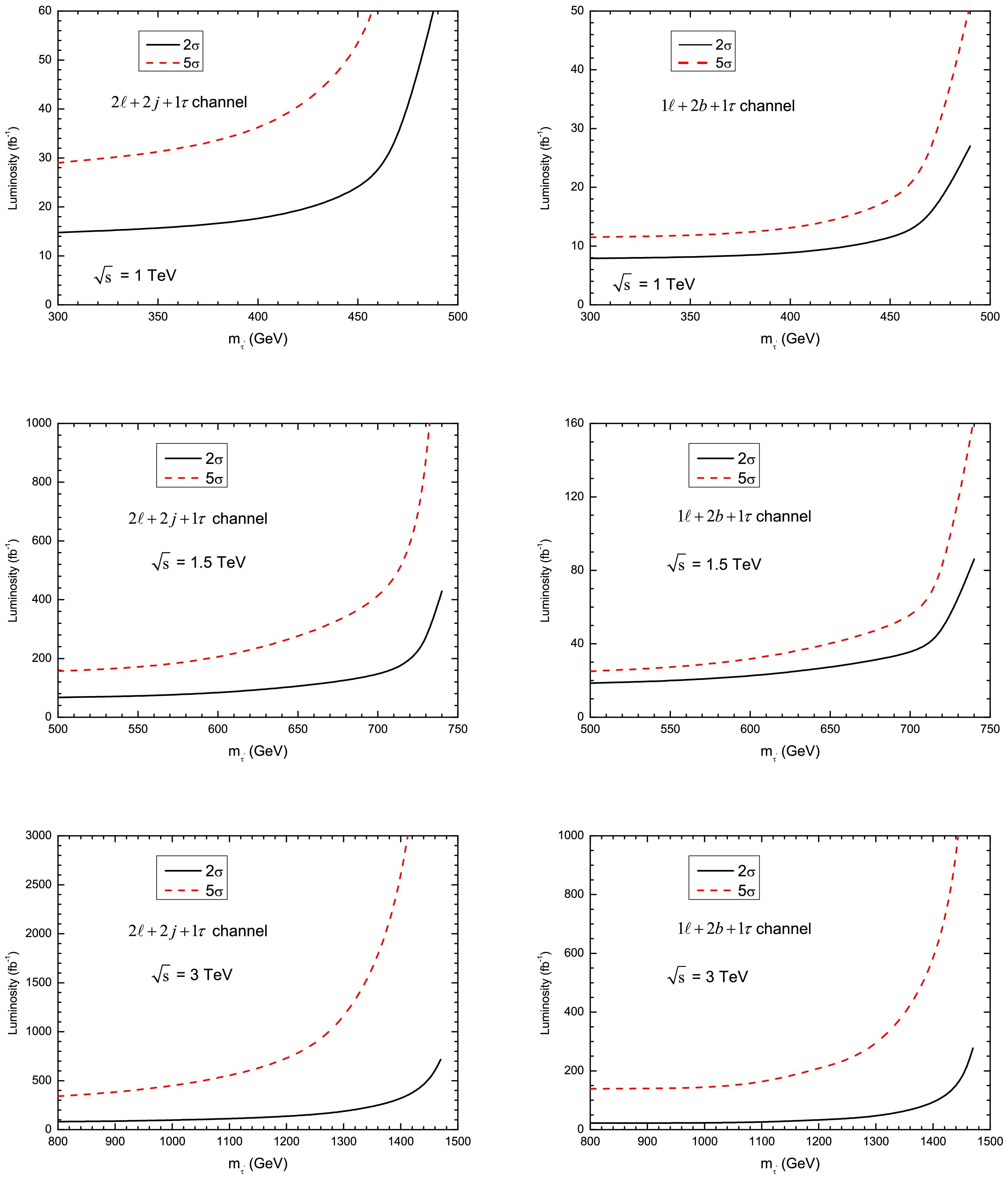

Figure 6.  (color online) 2σ exclusion limit and $ 5\sigma $ discovery prospects contour plots for case 1 (left) and case 2 (right) with c.m. energies of $ \sqrt{s}=1 $ TeV, 1.5 TeV, and 3 TeV.

In this work, we present a comprehensive study of the production and detection of weak isosinglet vector-like leptons (VLLs) at future high-energy $ e^+e^- $ colliders. Our analysis focuses on center-of-mass energies of $ \sqrt{s} = 1\; \mathrm{TeV} $, $ 1.5\; \mathrm{TeV} $, and $ 3\; \mathrm{TeV} $, leveraging polarized beams to maximize discovery potential.

A detailed investigation of the $ 2\ell+2j+1\tau+\not{E}_T $ and $ 1\ell+2b+1\tau+\not{E}_T $ final states demonstrates that optimized selection criteria can suppress SM backgrounds to $ \mathcal{O}(10^{-3}-10^{-4}) $ fb while preserving signal efficiency. Notably, the $ 1\ell+2b+1\tau+\not{E}_T $ channel emerges as the most promising signature for both exclusion and discovery of singlet VLLs at $ e^+e^- $ colliders, owing to its enhanced production cross sections and significantly reduced SM background contamination.

The projected $ 5\sigma $ discovery reaches are:

● $ m_{\tau^\prime} \lesssim 490\; \mathrm{GeV} $ at $ \sqrt{s} = 1\; \mathrm{TeV} $ with $ 50\; \mathrm{fb}^{-1} $

● $ m_{\tau^\prime} \lesssim 740\; \mathrm{GeV} $ at $ \sqrt{s} = 1.5\; \mathrm{TeV} $ with $ 160\; \mathrm{fb}^{-1} $

● $ m_{\tau^\prime} \lesssim 1440\; \mathrm{GeV} $ at $ \sqrt{s} = 3\; \mathrm{TeV} $ with $ 1000\; \mathrm{fb}^{-1} $

These limits substantially exceed the current LHC sensitivity of $ m_{\tau^\prime} \sim 150\; \mathrm{GeV} $ for singlet VLLs. Our results underscore the unique capability of $ e^+e^- $ colliders as precision instruments for BSM physics searches, particularly for VLL studies, where their clean experimental environment and beam polarization provide unparalleled advantages over hadron colliders.

While the hadronic decays of boosted objects (e.g., $ W \to jj $ and $ h \to b\bar{b} $) produce highly collimated jets that can merge into single fat jets, this analysis specifically focuses on resolved two-jet topologies. A comprehensive investigation of the extreme boost regime, employing dedicated fat jet algorithms with large resolution parameters ($ R \geq 1.0 $) and substructure techniques, will be systematically examined in a subsequent study. On the other hand, in the regime of sufficiently small mixing parameters $ \epsilon $, the singlet vector-like leptons (VLLs) may exhibit long-lived particle characteristics due to their suppressed decay widths, as demonstrated in recent LHC studies [50, 51]. The investigation of this long-lived $ \tau' $ scenario, involving displaced vertex signatures and time-dependent detection methods at the future CLIC is beyond the scope of this work and will be discussed in more detail in future studies.

Take the case for $\sqrt{s}=1$ TeV, the effects of initial state radiation (ISR) and beam polarization are considered in MadGraph5_aMC_v3.3.2 by adding the following commands in the run_card:

set lpp1 +3

set lpp2 -3

set pdlabel isronlyll

set polbeam1 +80

set polbeam2 -20

where the beam polarization is set from -100 (left-handed) to 100 (right-handed). For $\sqrt{s}=3$ TeV at the CLIC, the following commands are added in the run_card:

set lpp1 +3

set lpp2 -3

set pdlabel clic3000ll

set polbeam1 +80

set polbeam2 0