


 Abstract
 HTML
HTML Reference
 Related
 PDF
PDF


-
In the past couple of decades, a growing number of new hadron states have been observed experimentally, and investigations of the nature of these new states have become one of the most intriguing topics in hadron physics. Among these new hadron states, some are difficult to assign as conventional mesons or baryons, and they are thus considered good candidates for QCD exotic states, such as hadronic molecular states, compact multiquark states, and hybrid states (for recent reviews, we refer to Refs. [1-11]).
Very recently, the LHCb collaboration observed two new states,
$ X_0(2900) $ and$ X_1(2900) $ , in the$ K^+D^- $ invariant mass distribution of$ B^+ \to D^+ D^- K^+ $ . The resonance parameters of these two states are reported to be [12]:$ \begin{aligned}[b] m_{X_0(2900)} =& (2866\pm 7) \ \mathrm{MeV}, \\ \Gamma_{X_0(2900)} =& (57.2 \pm 12.9) \ \mathrm{MeV}, \\ m_{X_1(2900)} =& (2904\pm 5) \ \mathrm{MeV}, \\ \Gamma_{X_1(2900)} =& (110.3 \pm 11.5) \ \mathrm{MeV}. \end{aligned} $

(1) The
$ J^P $ quantum numbers of$ X_0(2900) $ and$ X_1(2900) $ are$ 0^+ $ and$ 1^- $ , respectively [12].Since
$ X_0(2900) $ and$ X_1(2900) $ are observed in the$ K^+D^- $ channel, the only possible quark components of these states are$ u d \bar{c} \bar{s} $ , which indicates that they are composed of quarks with four different flavors. Such states are particularly interesting since they obviously cannot be assigned as a conventional hadron. In 2016, another similar structure,$ X(5568) $ , was reported by the D0 collaboration in the$ B_s \pi $ invariant mass distribution, which is also a fully open flavor state [13]. However, after the observation of the D0 collaboration, the LHCb, CMS, CDF, and ATLAS collaborations negated the existence of$ X(5568) $ [14-17]. Thus, the present observation of$ X_0(2900) $ and$ X_1(2900) $ has brought attention back to the existence of fully open flavor states.Considering four different flavor quark components of
$ X_0(2900) $ and$ X_1(2900) $ , one can naturally consider these states as tetraquark candidates. In Ref. [18], the mass spectrum of exotic tetraquark states with four different flavors is investigated by using a color-magnetic interaction model, and the masses of states with$ I(J^P) = 1(0^+) $ are reported as 2607 and 3129 MeV, while those with$ I(J^P) = 0(0^+) $ are 2320 and 2850 MeV. After the observation of$ X_0(2900) $ and$ X_1(2900) $ , the authors of Refs. [19, 20] indicated that the$ X_0(2900) $ can be an isosinglet compact tetraquark state, while the estimations in Ref. [21] indicate that the$ X_0(2900) $ should be a radial excited tetraquark with$ J^P = 0^+ $ . As for$ X_0(2900) $ , the investigations in Refs. [21, 22] support that the$ X_1(2900) $ can be assigned as a$ P$ -wave compact diquark-antidiquark tetraquark state. However, the calculations in an extended relativized quark model indicate that the predicted mass of$ 0^+ $ $ ud\bar{s}\bar{c} $ is different from that of the$ X_0(2900) $ , which disfavors the assignment of the$ X_0(2900) $ as a compact tetraquark [23].It should be noticed that in the vicinity of 2900 MeV, there are abundant thresholds of charmed and strange mesons, such as
$ K^\ast D^\ast $ ,$ KD_1 $ , and$ KD_0 $ . In Refs. [24, 25], the possible molecular states composed of (anti-)charmed and strange mesons have been investigated. Considering the$ J^P $ quantum numbers of$ X_0(2900) $ and$ X_1(2900) $ , the former can result from the$ K^\ast \bar{D}^\ast $ interaction, while the latter can result from the$ K\bar{D}_1 $ interaction. In Ref. [26], the structure corresponding to$ X_0(2900) $ and$ X_1(2900) $ can be interpreted as the triangle singularity. In Ref. [27], the estimation from the one-boson exchange model indicates that the interactions of$ K^\ast \bar{D}^\ast $ are strong enough to form a molecular state. Thus,$ X_0(2900) $ can be interpreted as a$ K^\ast \bar{D}^\ast $ molecular state. Such an interpretation is also supported by the estimations in Refs. [22, 28].In molecular interpretations, we construct the one-boson-exchange potential of
$ K^\ast \bar{D}^\ast $ and$ K\bar{D}_1 $ interactions. The scattering amplitude can be obtained with the help of the quasipotential Bethe-Salpeter equation (qBSE) from the interaction potentials, and the poles of the scattering amplitudes are searched for in the complex energy plane. In the current work, both bound and virtual states will be considered in the calculation to discuss the relation between the experimentally observed states$ X_0(2900)/ $ $ X_1(2900) $ and the$ K^\ast \bar{D}^\ast/K\bar{D}_1 $ interactions.This work is organized as follows. We present the formalism used in the present estimation in the following section. The numerical results and related discussions are given in Section III, and the last section is devoted to a short summary.
-
In the current work, we will consider two interactions, the
$ K^*\bar{D}^* $ and$ K\bar{D}_1 $ interactions. The possible isospins of the states composed by$ K^*\bar{D}^* $ and$ K\bar{D}_1 $ could be 0 and 1, and the corresponding flavor functions are$ \begin{aligned}[b] | K^\ast \bar{D}^{\ast}, I = 0 \rangle =& \frac{1}{\sqrt{2}} \left[ K^{\ast+} D^{\ast -} - K^{\ast 0} \bar{D}^{\ast 0}\right],\\ | K^\ast \bar{D}^{\ast}, I = 1 \rangle =& \frac{1}{\sqrt{2}} \left[ K^{\ast+} D^{\ast -} + K^{\ast 0} \bar{D}^{\ast 0}\right] , \\ | K \bar{D}_1, I = 0 \rangle =& \frac{1}{\sqrt{2}} \left[ K^+ D_1^- - K^{0} \bar{D}_1^{ 0}\right],\\ | K \bar{D}_1, I = 1 \rangle =& \frac{1}{\sqrt{2}} \left[ K^+ D_1^- + K^{0} \bar{D}_1^{ 0}\right].\end{aligned} $

(2) In the one-boson-exchange model, the
$ K^* $ meson and$ \bar{D}^* $ meson interact by exchanging$ \pi $ ,$ \eta $ ,$ \rho $ , and$ \omega $ mesons. For the$ K\bar{D}_1 $ interaction, the$ \pi $ and$ \eta $ exchanges are forbidden, and only vector exchanges are allowed. Here, the vector exchanges are included explicitly, so we do not consider the contact terms as discussed in Refs. [29-33]. To describe the interaction, we need the effective Lagrangians at two vertices. For the charmed meson part, the effective Lagrangians can be written with the help of heavy quark and chiral symmetries as [34-38]$ \begin{aligned}[b] \mathcal{L}_{\mathcal{P}^*\mathcal{P}^*\mathbb{P}} =& \frac{2g}{f_\pi}\epsilon_{\mu\nu\alpha\beta} \tilde{\mathcal{P}}^{*\mu}_a\tilde{\mathcal{P}}^{*\nu\dagger}_bv^\alpha \partial^\beta\mathbb{P}_{ba},\\ \mathcal{L}_{\mathcal{P}^*\mathcal{P}^*\mathbb{V}} =& -\sqrt{2}\beta g_V \tilde{\mathcal{P}}^*_a\cdot\tilde{\mathcal{P}}_b^{*\dagger}\; v\cdot\mathbb{V}_{ba}\\& +{\rm i}2\sqrt{2}\lambda g_V \tilde{\mathcal{P}}^{*\mu}_a\tilde{\mathcal{P}}^{*\nu\dagger}_b(\partial_\mu\mathbb{V}_\nu-\partial_\nu\mathbb{V}_\mu)_{ba}, \\ \mathcal{L}_{\mathcal{P}_1\mathcal{P}_1\mathbb{V}} =& -\sqrt{2}\beta_2 g_V \tilde{\mathcal{P}}_{1a}\cdot \tilde{\mathcal{P}}^{\dagger}_{1b}\; v\cdot \mathbb{V}_{ba}\\ & -\frac{5\sqrt{2}{\rm i}\lambda_2 g_V}{3}\tilde{\mathcal{P}}^\mu_{1a}\tilde{\mathcal{P}}^{\nu\dagger}_{1b}(\partial _\mu\mathbb{V}_{\nu}-\partial_\nu\mathbb{V}_\mu)_{ba},\end{aligned} $

(3) where the velocity
$ v $ should be replaced by$ {\rm i}\overleftrightarrow{\partial}/\sqrt{m_im_f} $ , with$ m_{i,f} $ being the mass of the initial or final heavy meson.$ \tilde{\mathcal{P}} = (\bar{D}^0,D^-,D_s^-) $ and$ \tilde{\mathcal{P}}^* = (\bar{D}^{*0},D^{*-},D_s^{*-}) $ satisfy the normalization relations$ \langle 0|\tilde{\mathcal{P}}|\bar{Q}{q}(0^-)\rangle = \sqrt{M_{\tilde{\mathcal{P}}}} $ and$ \langle 0|\tilde{\mathcal{P}}^*_\mu|\bar{Q}{q}(1^-)\rangle = \epsilon_\mu\sqrt{M_{\tilde{\mathcal{P}}^*}} $ .$ \mathbb P $ and$ \mathbb V $ are the pseudoscalar and vector matrices:$\begin{aligned}[b] {\mathbb P} =& \left(\begin{array}{*{20}{c}} \dfrac{\sqrt{3}\pi^0+\eta}{\sqrt{6}}&\pi^+&K^+\\ \pi^-&\dfrac{-\sqrt{3}\pi^0+\eta}{\sqrt{6}}&K^0\\ K^-&\bar{K}^0&-\dfrac{2\eta}{\sqrt{6}} \end{array}\right),\\ \mathbb{V} =& \left(\begin{array}{*{20}{c}} \dfrac{\rho^0+\omega}{\sqrt{2}}&\rho^+&K^{*+}\\ \rho^-&\dfrac{-\rho^{0}+\omega}{\sqrt{2}}&K^{*0}\\ K^{*-}&\bar{K}^{*0}&\phi\end{array} \right),\end{aligned} $

(4) which correspond to
$ (\bar{D}^0,D^-,D_s^-) $ . The coupling constants have been determined in the literature with the heavy quark symmetry and available experimental data:$ g = 0.59 $ ,$ \beta = 0.9 $ ,$ \lambda = 0.56 $ ,$ \beta_2 = 1.1 $ , and$ \lambda_2 = -0.6 $ , with$ g_V = 5.9 $ and$ f_\pi = 0.132 $ GeV [39-44].To describe the couplings of the
$ K^{(*)} $ meson with exchanged pseudoscalar and/or vector mesons, the effective Lagrangians used are:$ \begin{aligned}[b] {\cal L}_{KKV} = &-{\rm i}g_{KKV} \; KV^\mu \partial_\mu K+{\rm H.c.},\\ {\cal L}_{K^*K^*V} =& {\rm i}\frac{g_{K^*K^*V}}{2}( K^{*\mu\dagger}{V}_{\mu\nu}K^{*\nu}+K^{*\mu\nu\dagger}{V}_{\mu}K^{*\nu}\\&+K^{*\mu\dagger}{V}_{\nu}K^{*\nu\mu}),\end{aligned} $

$ \begin{aligned}[b] {\cal L}_{K^*K^*P} =& g_{K^*K^*P}\epsilon^{\mu\nu\sigma\tau}\partial^\mu K^{*\nu} \partial_\sigma P K^{*\tau}+{\rm H.c.}, \end{aligned} $

(5) where
$ K^{*\mu\nu} = \partial^\mu K^{*\nu}-\partial^\nu K^{*\mu} $ . The flavor structures are$ K^{*\dagger}{\mathit{\boldsymbol{A}}}\cdot { \tau} K^* $ for an isovector A ($ = \pi $ or$ \rho $ ) meson, and$ K^{*\dagger} K^* B $ for an isoscalar B ($ = \eta $ ,$ \omega $ ) meson. With the help of the SU(3) symmetry, the coupling constants can be obtained from the$ \rho\rho\rho $ and$ \rho\omega\pi $ couplings.$ g_{\rho\rho\rho} $ is suggested to be equivalent to$ g_{\pi\pi\rho} = 6.2 $ , and$ g_{\omega\pi\rho} = 11.2 $ GeV$ ^{-1} $ [45-47]. The SU(3) symmetry suggests$ g_{K^*K^*\rho} = g_{K^*K^*\omega} = $ $ g_{\rho\rho\rho}/(2\alpha) $ , and$ g_{K^*K^*\pi} = g_{K^*K^*\eta}/[-\sqrt{1/3}(1-4\alpha)] = g_{\omega\rho\pi}/(2\alpha) $ with$ \alpha = 1 $ [48-51].In fact, the above vertices have been applied to study many XYZ particles and hidden-strange molecular states [44, 49-54]. Hence, in the current work, we only need to reconstruct the vertices
$ \Gamma_{1,2} $ for charmed or strange mesons to the potential considered here as$ {\cal V}_{\mathbb{P}} = I_{\mathbb{P}}\Gamma_1\Gamma_2 P_{\mathbb{P}}f_\mathbb{P}^2(q^2),\;\;\ \ {\cal V}_{\mathbb{V}} = I_{\mathbb{V}}\Gamma_{1\mu}\Gamma_{2\nu} P^{\mu\nu}_{\mathbb{V}}f_\mathbb{V}^2(q^2), $

(6) where the propagators are defined as usual as
$ P_{\mathbb{P}} = \frac{\rm i}{q^2-m_{\mathbb{P}}^2},\;\;\ \ P^{\mu\nu}_\mathbb{V} = {\rm i}\frac{-g^{\mu\nu}+q^\mu q^\nu/m^2_{\mathbb{V}}}{q^2-m_\mathbb{V}^2}, $

(7) and we adopt a form factor
$ f_{\mathbb{P},\mathbb{V}}(q^2) $ to compensate the off-shell effect of the exchanged meson as$ f_e(q^2) = $ $ {\rm e}^{-(m_e^2-q^2)^2/\Lambda_e^2} $ , with$ m_e $ being$ m_{\mathbb{P},\mathbb{V}} $ and q being the momentum of the exchanged meson. This treatment also reflects the non-pointlike nature of the constituent mesons. The cutoff is rewritten in the form of$ \Lambda_e = m_e+\alpha_e\; \Lambda_{\rm QCD} $ , with$ \Lambda_{\rm QCD} $ being the scale of QCD and taken as 0.22 GeV [55]. The flavor factors$ I_{\mathbb{P},\mathbb{V}} $ for certain meson exchange and total isospin are presented in Table 1.$ I_\pi $ 

$ I_\eta $ 

$ I_\rho $ 

$ I_\omega $ 

$ I=0 $ 

$ -3\sqrt{2}/2 $ 

$ {1}/{\sqrt{6}} $ 

$ -3\sqrt{2}/2 $ 

$ {1}{\sqrt{2}} $ 

$ I=1 $ 

$ \sqrt{2}/2 $ 

$ {1}/{\sqrt{6}} $ 

$ \sqrt{2}/2 $ 

$ {1}/{\sqrt{2}} $ 

Table 1. Flavor factors
$ I_{\mathbb{P},\mathbb{V}} $ for certain meson exchange and total isospin. The$ \pi $ and$ \eta $ exchanges are forbidden for the$ K\bar{D}_1 $ interaction.With the potential, the scattering amplitude can be obtained with the qBSE [56-58]. The qBSE with fixed spin-parity
$ J^P $ is written as [29, 50, 59]$ \begin{aligned}[b] {\rm i}{\cal M}^{J^P}_{\lambda'\lambda}({p}',{p}) =\;& {\rm i}{\cal V}^{J^P}_{\lambda',\lambda}({p}',{ p})+\sum_{\lambda''}\int\frac{{ p}''^2{\rm d}{p}''}{(2\pi)^3}\\ &\times{\rm i}{\cal V}^{J^P}_{\lambda'\lambda''}({p}',{p}'') G_0({p}''){\rm i}{\cal M}^{J^P}_{\lambda''\lambda}({p}'',{p}), \end{aligned} $

(8) where the sum extends only over nonnegative helicity
$ \lambda'' $ .$ G_0({p}'') $ is reduced from the 4-dimensional propagator by the spectator approximation, and in the center-of-mass frame with$ P = (W,{ 0}) $ it reads$ G_0({p}'') = \frac{1}{2E_h({p''})[(W-E_h({ p}''))^2-E_l^{2}({p}'')]}. $

(9) Here, as required by the spectator approximation, the heavier meson (
$ h = \bar{D}^*,\bar{D}_1 $ ) is on-shell, which satisfies$ p''^0_h = E_{h}({p}'') = \sqrt{ m_{h}^{\; 2}+ p''^2} $ .$ p''^0_l $ for the lighter meson ($ l = K^*, K $ ) is then$ W-E_{h}({ p}'') $ . A definition of$ {p} = |{ p}| $ is adopted here. The partial-wave potential is defined with the potential of the interaction obtained above as$ \begin{aligned}[b]{\cal V}_{\lambda'\lambda}^{J^P}({p}',{p}) =& \;2\pi\int {\rm d}\cos\theta \; [{ d}^{J}_{\lambda\lambda'}(\theta) {\cal V}_{\lambda'\lambda}({ p}',{ p})\\& +\eta { d}^{J}_{-\lambda\lambda'}(\theta) {\cal V}_{\lambda'-\lambda}({ p}',{ p})],\end{aligned} $

(10) where
$ \eta = PP_1P_2(-1)^{J-J_1-J_2} $ , with P and J being parity and spin for the system,$ K^*/K $ meson or$ \bar{D}^*/\bar{D}_1 $ meson. The initial and final relative momenta are chosen as$ { p} = (0,0,{p}) $ and$ { p}' = ({p}'\sin\theta,0,{p}'\cos\theta) $ .$ d^J_{\lambda\lambda'}(\theta) $ is the Wigner d-matrix. In the qBSE approach, a form factor is introduced into the propagator to reflect the off-shell effect as an exponential regularization,$ G_{0}(p)\rightarrow G_{0}(p) $ $ [{\rm e}^{-(k^{2}_{1}-m^{2}_{1})^{2}/\Lambda^{4}_{r}}]^{2}, $ where$ k_{1} $ and$ m_{1} $ are the momentum and mass of the strange meson, respectively. The cutoff$ \Lambda_{r} $ is also parameterized as in the$ \Lambda_{e} $ case.$ \alpha_e $ and$ \alpha_r $ play analogous roles in the calculation of the binding energy. Hence, we take these two parameters as one parameter$ \alpha $ for simplicity [44]. This parameter is also used to absorb the uncertainties of our model, such as the inaccuracy of heavy quark and SU(3) symmetries in the Lagrangians. -
The scattering amplitude obtained above includes the variation of the energy of the system, W. After continuation of W to a complex energy z, the pole can be searched for in the complex energy z plane. The bound state corresponds to a pole at the real axis under threshold in the first Riemann sheet. If the attraction becomes weaker, the pole will move to the real axis under threshold in the second Riemann sheet, which corresponds to a virtual state [60]. In the current work, we will consider both bound and virtual states from the
$ K^*\bar{D}^* $ and$ K\bar{D}_1 $ interactions. -
In the current work, we will consider six states from the
$ K^*\bar{D}^* $ interaction with isospin$ I = (0, 1) $ , spin$ J = (0, 1, 2) $ , and parity$ P = + $ , which can be obtained in the S wave. In our model, the only free parameter is$ \alpha $ in the cutoff. Usually, a small value of$ \alpha $ should be chosen. For a cutoff$ \Lambda $ smaller than 3 GeV,$ \alpha $ should be smaller than 10. In the following, we present the results with$ \alpha $ in a larger range, from 1 to 20, for discussion. The results with very large$ \alpha $ are unreliable because it corresponds to a very small radius of the constituent hadrons. The results for the states from the$ K^*\bar{D}^* $ interaction are presented and compared with the experimentally observed$ X_0(2900) $ in Fig. 1 (here we use the term "virtual energy" to denote the deviation between the pole of a virtual state and the threshold).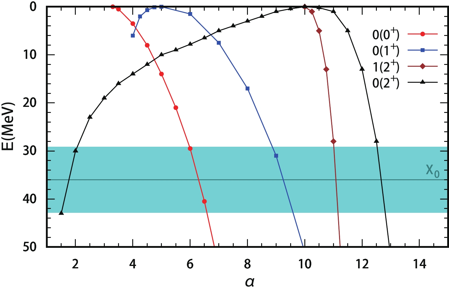
Figure 1. (color online) Binding or virtual energy E of bound or virtual states from the
$ K^*\bar{D}^* $ interaction with the variation of$ \alpha $ . Here$ E = M_{th}-W $ , with$ M_{th} $ and W being the threshold and mass of the state respectively. The circle, square, diamond, and triangle are for the states with$ I(J^P) = 0(0^+) $ ,$ 0(1^+) $ ,$ 1(2^+) $ , and$ 0(2^+) $ , respectively. The lines with the cyan bar are for the experimental mass and uncertainty, respectively, of the$ X_0(2900) $ state.Among the six states considered in the current work, four bound states can be produced from the
$ K^*\bar{D}^* $ interaction in the large range of$ \alpha $ considered here. The bound states with$ I(J^P) = 0(0^+) $ and$ 0(1^+) $ appear at small$ \alpha $ , about 4, and two bound states with$ 2^+ $ are found at$ \alpha $ larger than 10. Usually, a larger cutoff corresponds to a stronger interaction, which leads to larger binding energy for a bound state. The binding energies of the four bound states increase with increasing$ \alpha $ .Here, we also consider the possible virtual states from the interaction. Different from bound states, a virtual state leaves the threshold further with decreasing
$ \alpha $ and weakening of attraction. The bound state with$ I(J^P) = 0(2^+) $ appears at$ \alpha $ about 10, and the energy increases rapidly with the increase of$ \alpha $ . However, if we reduce$ \alpha $ , a pole can be found at the second Riemann sheet, and leaves the threshold with the decrease of$ \alpha $ . The pole moves to a position about 40 MeV below the threshold at$ \alpha $ about 2, and disappears there. No virtual state can be found for the case with$ 0(0^+) $ and$ 1(2^+) $ if we reduce$ \alpha $ . For the$ 0(1^+) $ case, a virtual state is also found, but it disappears very rapidly with the decrease of$ \alpha $ .Among the four bound states produced from the
$ K^*\bar{D}^* $ interaction, two bound states with$ 0(0^+) $ and$ 0(1^+) $ require a small value of$ \alpha $ . For the$ 0(2^+) $ state, only a virtual state can be produced with small$ \alpha $ . Since the$ X_{0}(2900) $ and$ X_1(2900) $ were observed in the$ K^+D^- $ channel, the allowed quantum numbers are$ 0^+ $ and$ 1^- $ . Hence, the current results support the assignment of the$ X_0(2900) $ observed at LHCb as a$ 0(0^+) $ state from the$ K^*\bar{D}^* $ interaction. As shown in Fig. 1, the experimental mass of the$ X_0(2900) $ can be reproduced at$ \alpha $ about 6. With such a value of$ \alpha $ , a bound state with$ 0(1^+) $ and a virtual state with$ 0(2^+) $ can be also produced from the$ K^*\bar{D}^* $ interaction. -
The
$ X_1(2900) $ state cannot be reproduced from the$ K^*\bar{D}^* $ interaction in the S wave. Here we consider another system with a threshold close to the mass of$ X_1(2900) $ , the$ K\bar{D}_1 $ interaction. We will consider two states from the$ K\bar{D}_1 $ interaction with$ I = (0, 1) $ and$ J^P = 1^- $ , which can be obtained in the S wave. The results are presented in Fig. 2.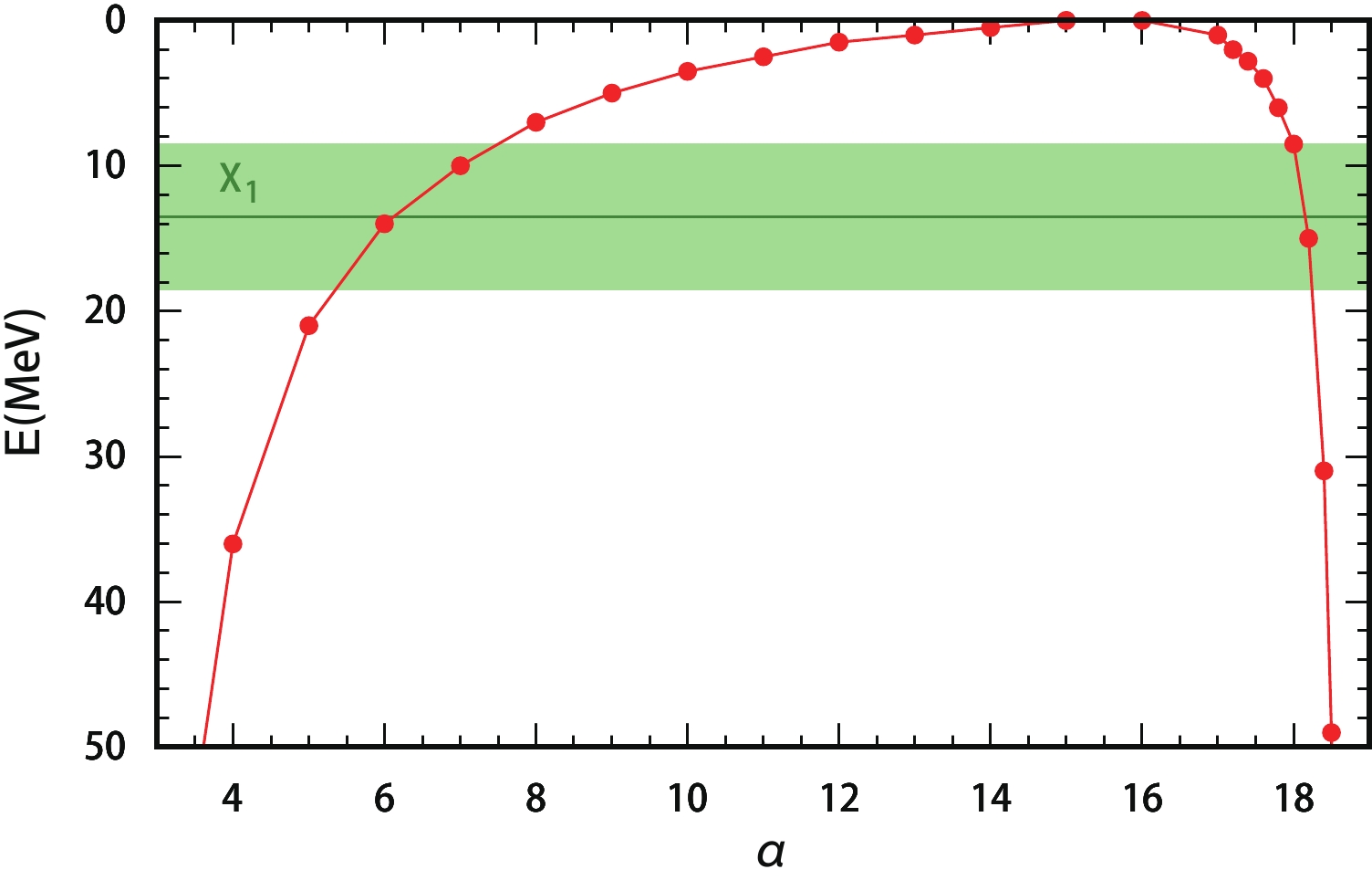
Figure 2. (color online) Virtual or binding energy E of the bound or virtual state from the
$ K\bar{D}_1 $ interaction with the variation of$ \alpha $ . The circles indicate the state with$ I(J^P) = 0(1^-) $ . The lines with the light green bar are for the experimental mass and uncertainty, respectively, of the$ X_1(2900) $ state. Other conventions are the same as in Fig. 1.Among these two states, only the isoscalar interaction is attractive. However, the bound state with
$ 0(1^-) $ appears at a very large$ \alpha $ value, about 16, which corresponds to a large cutoff$ \Lambda $ of about 4 GeV. It is unreliable to assign the$ X_1(2900) $ as a bound state. As with the$ 0(2^+) $ state of the$ K^*D^* $ interaction, if we decrease$ \alpha $ , a virtual state with$ 0(1^-) $ from the$ K\bar{D}_1 $ interaction can be found in a large range of$ \alpha $ , from about 4 to 16. Such a state can be related to the experimentally observed$ X_1(2900) $ . To reproduce the experimental mass of$ X_1(2900) $ , the value of$ \alpha $ should be chosen as about 6, which is also the value to reproduce the$ X_0(2900) $ . -
In the current work, inspired by the newly observed
$ X_{0,1}(2900) $ at LHCb, the$ K^*\bar{D}^* $ and$ K\bar{D}_1 $ interactions, which have thresholds about 2900 MeV, are studied in the qBSE approach. The bound and virtual states from the interaction are searched for as poles in the complex energy plane of the scattering amplitude, which is obtained from the one-boson-exchange potential.A bound state with
$ 0(0^+) $ is produced from the$ K^*\bar{D}^* $ interaction. The radius R of the bound state can be estimated as$ R\sim1/\sqrt{2\mu E_B} $ , with$ \mu $ and$ E_B $ being the reduced mass and binding energy [7]. The experimental binding energy, about 35 MeV, leads to a radius of about 1 fm for the$ K^*\bar{D}^* $ bound state. Considering that the constituent mesons have radii of about 0.5 fm, this supports the assignment of$ X_0(2900) $ as a$ K^*\bar{D}^* $ molecular state. The state with$ 0(0^+) $ from the$ K^*\bar{D}^* $ interaction has been suggested in many different approaches [22, 27, 28, 61].A virtual state with
$ 0(1^-) $ is also produced from the$ K\bar{D}_1 $ interaction, with a reasonable choice of parameter. Different from the assignment of$ X_0(2900) $ as a$ K^*\bar{D}^* $ state with$ 0(0^+) $ , the interpretation of$ X_1(2900) $ is under debate in the literature. In Ref. [62], a molecular state can be produced from the$ K\bar{D}_1 $ interaction by solving the Bethe-Salpeter equation. In Ref. [22], the$ X_1(2900) $ was interpreted as the P-wave$ \bar{c}\bar{s}ud $ compact tetraquark state with$ 1^- $ . In Ref. [27], the$ X_1(2900) $ cannot be explained as a molecular state from the interaction considered.These two states can decay into the
$ K^+D^- $ channel in S and P waves, so can be related to the$ X_{0}(2900) $ and$ X_1(2900) $ observed at LHCb, respectively. The$ X_0(2900) $ state, as an$ K^*\bar{D}^* $ molecular state, should be prone to separate to$ K^* $ and$ \bar{D}^* $ mesons. Considering that$ K^* $ and$ \bar{D}^* $ have decay widths of about 50 and$ <2 $ MeV, this gives the$ X_0(2900) $ , which is quite close to the experimental value. For the$ X_1(2900) $ states, the current study suggests that it is a virtual state. The virtual state is in the second Riemann sheet, which leads to a cusp at threshold, which may correspond to a larger width if we assume it is a resonance, which is also consistent with the experimental value larger than 100 MeV.Besides these two states, a bound state with
$ 0(1^+) $ and a virtual state with$ 0(2^+) $ are produced from the$ K^*\bar{D}^* $ interaction with a small$ \alpha $ value, about 6, which is also the value to reproduce the$ X_{0,1}(2900) $ . The mass order of the$ 0(0^+) $ and$ 0(1^+) $ states predicted in Ref. [27] is consistent with our results, and in both models, very large cutoff is required to produce a$ 0(2^+) $ bound state. In Ref. [28], masses of 2.722 and 2.866 GeV for the$ 0(1^+) $ state, and of 2.866 GeV for the$ 0(2^+) $ state, were predicted with the$ X_0(2900) $ as input. In Ref. [61], a different mass order was predicted: 2866,$ 2861 $ , and 2775 MeV for$ 0(0^+) $ ,$ 0(1^+) $ , and$ 0(2^+) $ , respectively, which follows their previous work in Ref. [25]. The low mass of the$ 2^+ $ state was also found in studies of$ f_J $ and$ D_J $ mesons [63, 64]. Such an explicit difference in the mass order may be from the explicit form and treatment of the interaction. More theoretical research and experimental searches for such states, especially the mass order of these states, will be helpful to understand the$ X(2900) $ .
Molecular picture for X0(2900) and X1(2900)
- Received Date: 2021-01-06
- Available Online: 2021-06-15
Abstract: Inspired by the newly observed


 DownLoad: