


 Abstract
 HTML
HTML Reference
 Related
 PDF
PDF


-
Matter-antimatter asymmetry [1] is a primary issue in the standard cosmology model. According to the Big Bang theory [2], matter and antimatter in the universe should be produced equally and exist in equal amounts. However, observations show that the number of baryons in the universe is
$ 10^9-10^{10} $ [3] times that of antibaryons. Sakharov proposed the three conditions to understand this puzzle [4], the first of which is that the baryon number conservation must be violated. Consequently, several baryon number violation (BNV) searches have been conducted at collider experiments and specially designed non-collider experiments, such as proton decay experiments; however, no positive results have been obtained. Many theories [5, 6] pointed out that if BNV occurs, the lepton number should also be violated (LNV). This provides another perspective on exploring the asymmetry between matter and antimatter in the universe.Conversely, neutrino oscillation experiments [7−10] show that neutrinos have tiny masses, which proves that the Standard Model (SM) cannot fully describe the neutrino sector. Some of the SM extensions believe that neutrinos may have majorana components whose particle and antiparticle are identical [11]. This may lead to LNV processes with
$ \Delta L=2 $ , such as neutrinoless double beta decay ($ 0\nu2\beta $ ) [12]. Although hadrons comprising first generation quarks have been well explored in$ 0\nu2\beta $ , constraints on the LNV process [13−18] suggest that searching for LNV with non-first generation quark decays at collider experiments would be necessary.Many recent collider experiments, such as NA62 [19], E865 [20], LHCb [21], CMS [22], ATLAS [23], CLEO [24] and BESIII [25], have searched for LNV processes. Among them, references [19, 20] reported LNV with second generation quark decays in K mesons. However, no significant evidence of a possible LNV effect has been observed yet. Complementary to those measurements, the study of LNV using ϕ decays is distinctive owing to the different phase space (PHSP) it explores. In this study, we analyze the
$ (1.0087\pm0.0044)\times10^{10} $ $ J/\psi $ data sample collected with the BESIII detector [26] operating at the BEPCII storage ring [27] to search for the SM forbidden LNV decay of$ \phi\to\pi^+\pi^+e^-e^- $ . The charge conjugate channel is always implied throughout this study. -
The BESIII detector [26] records symmetric
$ e^+e^- $ collisions provided by the BEPCII storage ring [27] in the center-of-mass energy range from 1.85 to 4.95 GeV, with a peak luminosity of$ 1.1 \times 10^{33}\;\text{cm}^{-2}\text{s}^{-1} $ achieved at$ \sqrt{s} = 3.773\;\text{GeV} $ . BESIII has collected large data samples in this energy region [28]. The cylindrical core of the BESIII detector covers 93% of the full solid angle and comprises a helium-based multilayer drift chamber (MDC), a plastic scintillator time-of-flight system (TOF), and a CsI(Tl) electromagnetic calorimeter (EMC), all enclosed in a superconducting solenoidal magnet providing a 1.0 T magnetic field. The magnetic field was 0.9 T in 2012, which affects 11% of the total$ J/\psi $ data. The solenoid is supported by an octagonal flux-return yoke with resistive plate counter muon identification modules interleaved with steel. The charged-particle momentum resolution at$ 1\; {\rm GeV}/c $ is 0.5%, and the specific ionization energy loss (dE/dx) resolution is 6% for electrons from Bhabha scattering. The EMC measures photon energies with a resolution of 2.5% (5%) at 1 GeV in the barrel (end cap) region. The time resolution in the TOF barrel region is 68 ps, while that in the end cap region is 110 ps. The end cap TOF system was upgraded in 2015 using multigap resistive plate chamber technology, providing a time resolution of 60 ps, which benefits 87% of the data used in this analysis [29].Simulated Monte Carlo (MC) samples produced with GEANT4-based [30] software, which includes the geometric description of the BESIII detector [31] and the detector response, are used to determine the detection efficiency and to estimate the background contributions. The simulation includes the beam-energy spread and initial-state radiation (ISR) in the
$ e^+e^- $ annihilation modeled with the generator KKMC [32, 33]. The inclusive MC simulation sample includes the production of the$ J/\psi $ resonance and the continuum processes incorporated in KKMC [32, 33]. The known decay modes are modeled with EVTGEN [34, 35] using world averaged branching fraction values [36], and the remaining unknown decays from the charmonium states with LUNDCHARM [37, 38]. Final-state radiation from charged final-state particles is incorporated with PHOTOS [39]. -
In this analysis, we search for the decay
$ \phi\to\pi^+\pi^+e^-e^- $ via$ J/\psi\to\phi\eta, \eta\to\gamma\gamma $ . In order to avoid the large uncertainty from$ {\cal{B}}(J/\psi\to\phi\eta) $ [36], which is approximately 11%, we measure the branching fraction of the signal decay$ \phi\to\pi^+\pi^+e^-e^- $ relative to that of the reference channel$ \phi\to K^+K^- $ via$ J/\psi\to\phi\eta $ .The branching fractions of
$ \phi\to \pi^+\pi^+ e^-e^- $ and$\phi\to K^+K^-$ can be written as$ \begin{aligned} \begin{split} {\cal{B}}(\phi \to\pi^+\pi^+e^-e^-)=\frac{N_{\pi^+\pi^+e^-e^-}^{\rm{net}}/\varepsilon_{\pi^+\pi^+e^-e^-}}{N^{\rm{tot}}\times {\cal{B}}(J/\psi\to\phi\eta)\times{\cal{B}}(\eta\to\gamma\gamma)}, \end{split} \end{aligned} $

(1) and
$ \begin{aligned} {\cal{B}}(\phi \to K^+K^-)= \frac{N_{K^+K^-}^{\rm{net}}/\varepsilon_{K^+K^-}}{N^{\rm{tot}}\times {\cal{B}}(J/\psi\to\phi\eta)\times{\cal{B}}(\eta\to\gamma\gamma)}, \end{aligned} $

(2) respectively, where
$ N_{\pi^+\pi^+e^-e^-}^{\rm{net}} $ and$ N_{ K^+K^-}^{\rm{net}} $ are the signal yields,$ N^{\rm{tot}} $ is the total number of$ J/\psi $ events, and$ \varepsilon_{\pi^+\pi^+e^-e^-} $ and$ \varepsilon_{K^+K^-} $ are the detection efficiencies for the$ J/\psi\to\eta\phi, \eta\to\gamma\gamma,\phi\to\pi^+\pi^+e^-e^- $ and$ J/\psi\to\eta\phi,\eta\to\gamma\gamma,\phi\to K^+K^- $ , respectively.$ {\cal{B}}(J/\psi\to\phi\eta) $ and$ {\cal{B}}(\eta\to\gamma\gamma) $ are the branching fractions of$ J/\psi\to\phi\eta $ and$ \eta\to\gamma\gamma $ . Using the two equations above, the branching fraction of$ \phi\to \pi^+\pi^+ e^-e^- $ can be determined by$ \begin{aligned} {\cal{B}}(\phi \to\pi^+\pi^+ e^-e^-)={\cal{B}}(\phi\to K^+K^-) \times\frac{N_{\pi^+\pi^+e^-e^-}^{\rm{net}}/\varepsilon_{\pi^+\pi^+e^-e^-}}{N_{K^+K^-}^{\rm{net}}/\varepsilon_{K^+K^-}}, \end{aligned} $

(3) where
$ {\cal{B}}(\phi\to K^+K^-)=(49.2\pm0.5) $ % [36]. The total systematic uncertainty can be reduced significantly because the uncertainty of the input$ {\cal{B}}(\phi\to K^+K^-) $ is only 1.0%. -
The reference decay
$ J/\psi\to \phi\eta $ is reconstructed with$ \eta\to\gamma\gamma $ and$ \phi\to K^+K^- $ . In each event, at least two charged tracks and two neutral candidates are required.Charged tracks detected in the MDC are required to be within a polar angle (θ) range of
$ |{\rm{cos}}\theta|<0.93 $ , where θ is defined with respect to the z-axis, which is the symmetry axis of the MDC. The distance of closest approach to the interaction point (IP) must be less than 10 cm along the z-axis,$ |V_{z}| $ , and less than 1 cm in the transverse plane,$ |V_{xy}| $ . Events with exactly two good charged tracks with zero net charge are kept for further analysis. For charged particle identification (PID), we use a combination of the$ {\rm d}E/{\rm d}x $ in the MDC, and the time of flight in the TOF to calculate the Confidence Level (CL) for pion and kaon hypotheses ($ CL_{\pi} $ and$ CL_K $ ). For kaon candidates, they are required to satisfy$ CL_K>0.001 $ and$ CL_K>CL_{\pi} $ to avoid contamination from pions and to suppress background.The photon candidates are selected from isolated EMC clusters. The clusters are required to start within 700 ns after the event start time and fall outside a cone angle of
$ 20^\circ $ around the nearest extrapolated good charged track to suppress electronic noise and beam related background. The minimum energy of each EMC cluster is required to be greater than 25 MeV in the barrel region ($ |\cos\theta|<0.80 $ ) or 50 MeV in the end-cap regions ($ 0.86<|\cos\theta|<0.92 $ ). The η candidate is reconstructed by$ \eta \to \gamma \gamma $ , where the invariant mass of the$ \gamma \gamma $ pair is required to satisfy 0.45 GeV/$ {c}^2 $ $ < M_{\gamma \gamma} < $ 0.65 GeV/$ {c}^2 $ . A kinematic fit is performed to reduce backgrounds and improve mass resolution by constraining the total four momentum (4C) to that of the initial$ e^+e^- $ beams under the hypothesis of$ e^+e^-\to K^+K^-\gamma\gamma $ . All good photons are looped over together with the two tracks in the kinematic fit, and the candidate with the least$ \chi^2 $ is retained for further analysis.To obtain the signal yield of
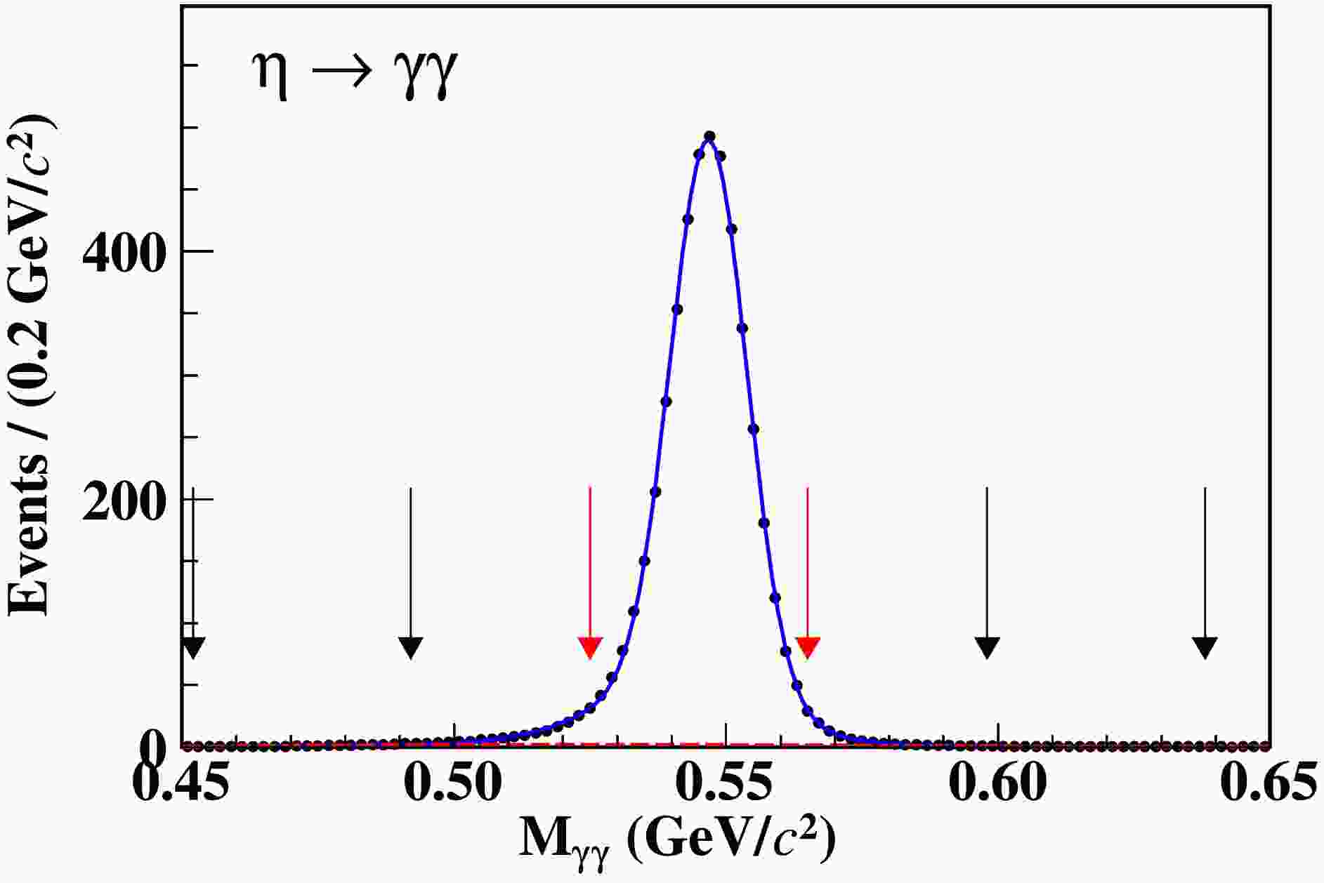
$ \phi\to K^+K^- $ , we fit the$ M_{K^+K^-} $ distribution of the accepted candidate events in the η signal region ([0.525,0.565] GeV/$ {c}^2 $ ) and in the η sideband region ([0.452,0.492] GeV/$ {c}^2 $ or [0.598,0.638] GeV/$ {c}^2 $ ). The signal region is determined by$ [\mu-3\sigma, \mu+3\sigma] $ ; the sideband region is outside the signal region and the distance between the two intervals is 5σ, where μ and σ are the mean and standard deviation obtained from a Gaussian fit to the$ M_{\gamma\gamma} $ distribution, as shown in Fig. 1. In the fits to the$ M_{K^+K^-} $ distribution in the η signal region, the signal shape is described by a MC shape convolved with a double Gaussian function and the background shape is described by second-order polynomial function. In the fits to the$ M_{K^+K^-} $ distribution in the η sideband region, the signal shape is described by a MC shape convolved with a double Gaussian function, and the background shape is described by an inverted ARGUS function [40] multiplied by a fourth-order polynomial function. The double Gaussian function and the background model parameters float in the fits. With the numbers of$ N_{\rm signal} $ and$ N_{\rm sideband} $ obtained from the fits in Fig. 2, the net number of the$ \phi\to K^+K^- $ candidate events is calculated by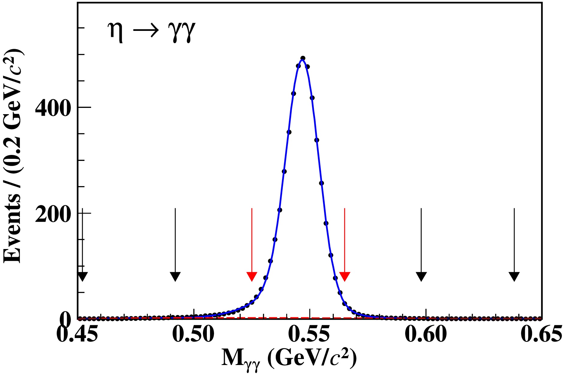
Figure 1. (color online) Fit to the
$ M_{\gamma\gamma} $ distribution, where the black points represent the signal MC candidates, the blue curve is the fit result, the red dashed line is the second-order polynomial background, the red arrows show the signal region, and the black arrows show the sideband region.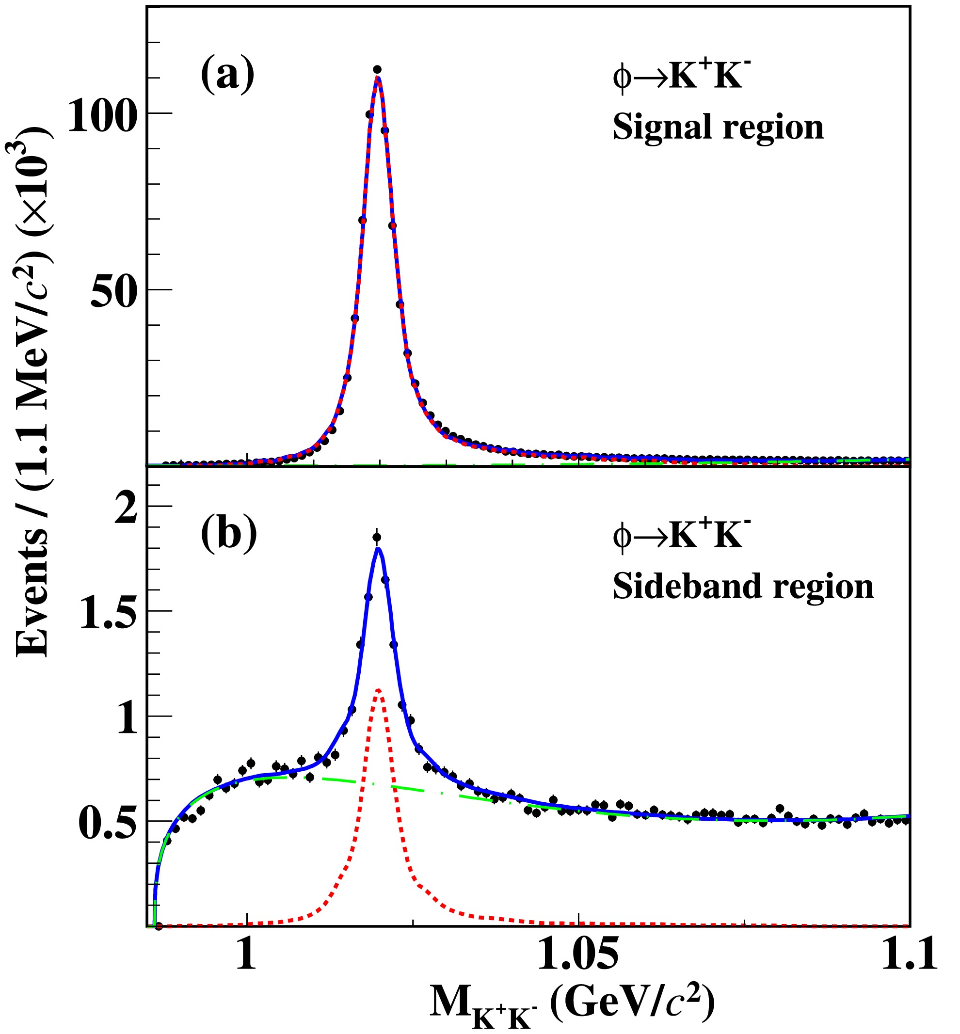
Figure 2. (color online) Invariant mass
$ M_{K^+K^-} $ distributions of$ J/\psi \to \phi \eta $ candidates in the (a) signal and (b) sideband region of η, with fit results overlaid. The black points represent the data, the blue curves are the fit results, the green dash-dotted curves are the fitted background shapes, and the red dotted curves are the signal shapes.$ \begin{aligned} N^{\rm net}_{K^+K^-}=N_{\rm signal}-\frac{1}{2}\times N_{\rm sideband}=823764\pm1023. \end{aligned} $

(4) Here,
$ \dfrac{1}{2}\times N_{\rm sideband} $ is the background yield under the$ M_{\gamma\gamma} $ signal region, where the scale factor of$ 1/2 $ is determined under the assumption that the background is flat in the$ M_{\gamma\gamma} $ distribution.To determine the detection efficiency, the
$ J/\psi\to \phi\eta\; (\phi\to K^+K^-, \eta\to\gamma\gamma) $ decays are simulated, where the decays of$ J/\psi\to\phi\eta $ ,$ \phi\to K^+K^- $ , and$ \eta\to\gamma\gamma $ are modeled by a helicity amplitude generator HELAMP, a VSS model (decay of a vector particle to a pair of scalars), and a PHSP generator, respectively [41]. After applying all the selection criteria, we fit the invariant mass of the$ K^+K^- $ combination ($ M_{K^+K^-} $ ) for the survived signal MC events in the signal and sideband regions, respectively. In the fits, the signal shape is modeled by a MC shape convolved with a double Gaussian function and the background is described by a second-order polynomial function. The number of observed signal events is obtained to be$N^{\rm MC}_{\rm obs}= N_{\phi\to K^+K^-}^{\rm signal}-\dfrac{1}{2}\times N_{\phi\to K^+K^-}^{\rm sideband}$ , where$ N_{\phi\to K^+K^-}^{\rm signal} $ and$ N_{\phi\to K^+K^-}^{\rm sideband} $ are the observed numbers in the η signal and sideband regions, respectively. Dividing it by the number of total signal MC events$ N^{\rm MC}_{\rm total} $ , the efficiency of detecting the decays of$ \phi\to K^+K^- $ is$ \begin{aligned} \varepsilon_{KK} = \frac{N^{\rm MC}_{\rm obs}}{N^{\rm MC}_{\rm total}}=\frac{471297}{1000000}=(47.1\pm0.1)\%. \end{aligned} $

(5) -
The LNV decay of
$ \phi \to \pi^+\pi^+e^-e^- $ is searched through$ J/\psi\to \phi\eta $ , where the η candidate is reconstructed through$ \eta\to\gamma\gamma $ . In each event, at least four charged tracks and two neutral candidates are required.The good charged tracks are selected using the same criteria as those used in the reference mode. For charged PID, we use a combination of the dE/dx in the MDC, the time of flight in the TOF, and the energy and shape of clusters in the EMC to calculate the CL for the electron, pion, and kaon hypotheses (
$ CL_e $ ,$ CL_{\pi} $ , and$ CL_K $ ). The electron candidates are required to satisfy$ CL_e>0.001 $ and$ CL_e/(CL_e+ CL_K+CL_{\pi})>0.8 $ . Furthermore, to suppress background from pions, electrons must satisfy an additional requirement$ E/p > 0.8 $ for tracks with$ p_e \geq $ 0.5 GeV/c, where E and p represent the energy deposited in the EMC and the momentum reconstructed in the MDC, respectively. Pion candidates are required to satisfy$ CL_\pi>0 $ and$ CL_\pi>CL_K $ . The good photons are selected in the same way as in the reference mode.A kinematic fit is performed to reduce backgrounds and improve the mass resolution by constraining the total four momentum (4C) to that of the initial
$ e^+e^- $ beams. All the good photons are looped over together with the four tracks in the kinematic fit. To suppress the combinatorial background, the$ \chi^2 $ of the 4C kinematic fit is required to be less than 30, determined via the Punzi significance method [42] using the formula$ \dfrac{\varepsilon}{1.5+\sqrt{B}} $ , where ε is the detection efficiency and B is the number of background events from the inclusive MC sample. If more than one combination is obtained, the combination with the minimum$ \chi^2 $ is retained.We perform 4C kinematic fits under six different hypotheses of
$ J/\psi \to \pi^+\pi^+e^-e^-\gamma\gamma $ ,$ K^+K^-K^+K^-\gamma\gamma $ ,$ K^+K^- p\bar p\gamma\gamma $ ,$ K^+K^-\pi^+\pi^-\gamma\gamma $ ,$ \pi^+\pi^-\pi^+\pi^-\gamma\gamma $ , and$ \pi^+\pi^-p\bar p\gamma\gamma $ to suppress the contamination of the final states with four charged tracks from mis-identification. If the kinematic fit for the$ \pi^+\pi^+e^-e^-\gamma\gamma $ hypotheses is successful and gives the minimum$ \chi^2 $ among these six assignments, the event is then accepted for further analysis.To further suppress possible background from
$ \gamma $ -conversion, the opening angle$ \theta_{\pi e} $ between any pions (possibly mis-identified from real positrons) and electrons are required to be greater than$ 8^\circ $ .Based on a fit with a double Gaussian function and a Chebychev polynomial to model the signal and background shapes of the simulated
$ M_{\pi^+\pi^+ e^-e^-} $ and$ M_{\gamma\gamma} $ distributions, the signal region is determined to be$ [0.99, 1.04] $ GeV/$ {c}^2 $ for$ M_{\pi^+\pi^+ e^-e^-} $ and$ [0.52, 0.57] $ GeV/$ {c}^2 $ for$ M_{\gamma\gamma} $ . This corresponds to a range of$ \pm3 $ times the mass resolution around their known masses [36]. The detection efficiency is determined to be 4.40% with simulated$J/\psi\to \phi\eta \to (\pi^+\pi^+e^-e^-)(\gamma\gamma)$ events, where the$ J/\psi $ decay is modeled by a helicity amplitude generator HELAMP [41] and the ϕ/η decays are modeled by a phase space (PHSP) generator.Using TopoAna, an event type analysis tool [43], the backgrounds from
$ J/\psi $ decays are investigated using an inclusive MC simulation sample, which has the same size as the$ J/\psi $ data sample. Only 39 events from 14 different decay channels remain. The distribution of$ M_{\pi^+\pi^+ e^-e^-} $ for the background events from the inclusive MC simulation sample is shown in Fig. 3, where the red arrows show the signal region. No background event is observed in the signal region.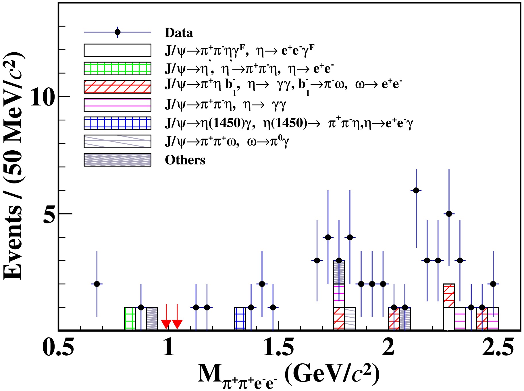
Figure 3. (color online) The distribution of
$ M_{\pi^+\pi^+ e^-e^-} $ for events in the range of$ M_{\gamma\gamma}\in(0.52,0.57) $ GeV/$ c^2 $ , where the points with error bars are data, the histogram in different styles represent different sources of background modes shown in the legends. The red arrows show the signal region.To avoid the influence of statistical fluctuation, large exclusive MC simulation samples for the three main background channels, (1)
$ J/\psi \to \pi^{+}\pi^-\eta\gamma^F,\eta \to e^{+}e^-\gamma^F $ ($ \gamma^F $ is the γ from final state radiation), (2)$ J/\psi \to\eta^{\prime}, ~ \eta^{\prime}\to\pi^{+}\pi^-\eta, \eta \to e^+e^- $ , and (3)$J/\psi \to \pi^{+}\eta b_{1}^{-},~\eta \to \gamma \gamma,~ b_{1}^{-}\to \pi^{-}\omega, \omega \to e^{+}e^-$ , are produced. Furthermore, the possibility of background from other ϕ decays, such as$J/\psi \to \phi \eta, \phi\to e^{+}e^-\eta, ~\eta \to \gamma \gamma$ , is also investigated. No background event is found near the signal region under the current MC sample statistics. Figure 4 shows the two dimensional distribution of$ M_{\gamma\gamma} $ versus$ M_{\pi^+ \pi^+ e^-e^-} $ of the accepted$ \phi \to \pi^+ \pi^+ e^-e^- $ candidate events in the data. No event is observed in the signal region.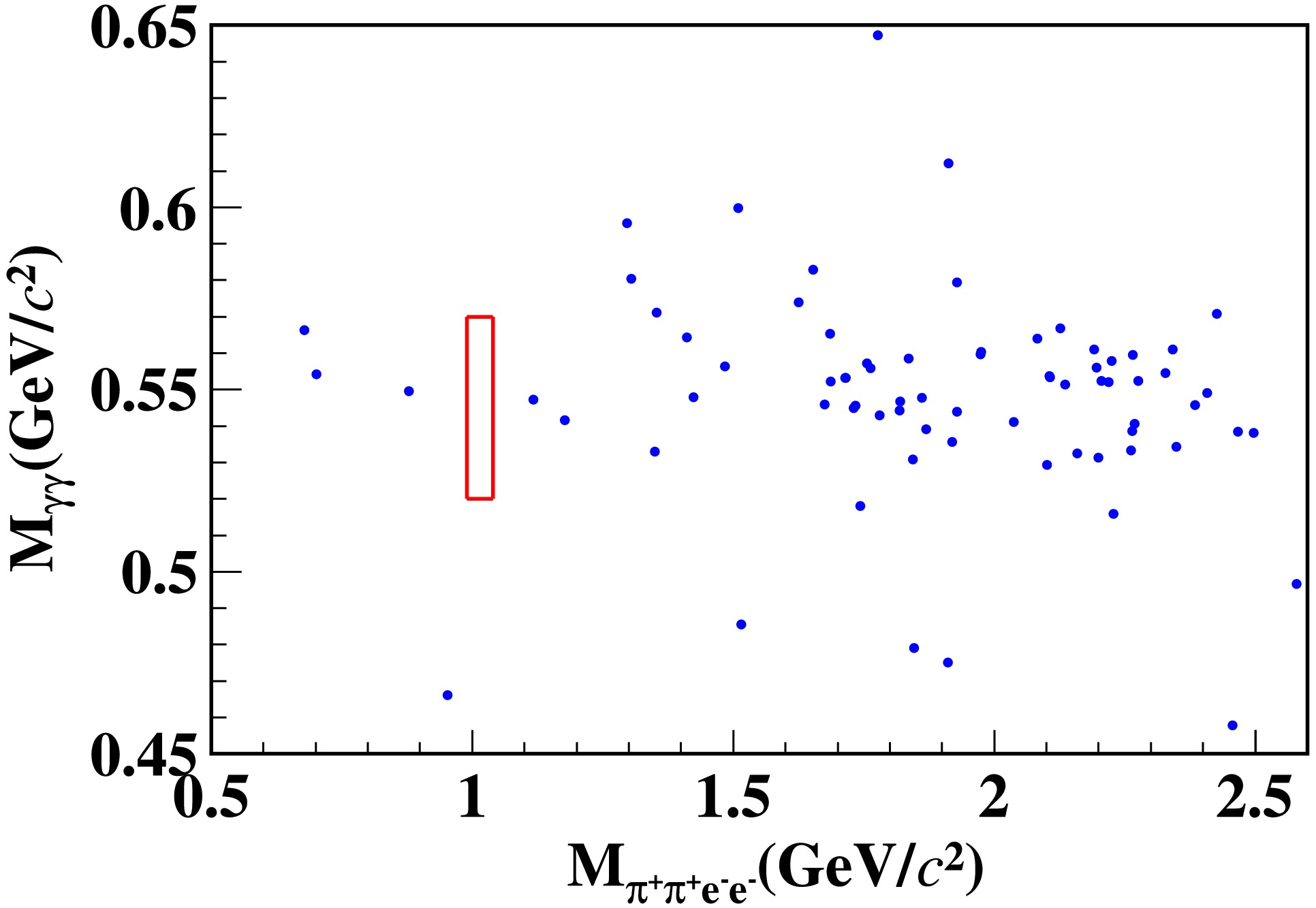
Figure 4. (color online) The distribution of
$ M_{\gamma\gamma} $ versus$ M_{\pi^+ \pi^+ e^-e^-} $ of the accepted$ \phi \to \pi^+ \pi^+ e^-e^- $ candidate events in data. The red box indicates the signal region defined as$ [0.99, 1.04] $ GeV/$ {c}^2 $ for$ M_{\pi^+\pi^+ e^-e^-} $ and$ [0.52, 0.57] $ GeV/$ {c}^2 $ for$ M_{\gamma\gamma} $ . -
The sources of systematic uncertainties for the product branching fractions include MDC tracking, charged PID, 4C kinematic fit,
$ \chi^2 $ requirement,$ \theta_{\pi e} $ requirement, signal window, fitting procedure, MC modeling,$ N^{\rm net}_{K^+K^-} $ determination, and$ {\cal{B}}(\phi\to K^+K^-) $ . All the systematic uncertainties are summarized in Table 1, and the total uncertainty is obtained by adding the individual components in quadrature.Source Uncertainty (%) MDC tracking 2.6 PID 6.2 4C kinematic fit for $ \phi\to K^+K^- $ 

0.2 4C kinematic fit for $ \phi\to \pi^+\pi^-e^+e^- $ 

2.3 $ \theta_{\pi e} $ selection requirement

4.1 Signal window 0.2 Yield of $ \phi\to K^+K^- $ 

1.1 MC modeling 1.9 $ {\cal{B}}(\phi\to K^+K^-) $ 

1.0 Total 8.6 Table 1. Relative systematic uncertainties in the branching fraction measurement.
The systematic uncertainties of photon detection and quoted branching fractions (
$ {\cal{B}}(J/\psi\to\phi\eta) $ and$ {\cal{B}}(\eta\to\gamma\gamma) $ ) are canceled based Eq. (3).The uncertainties in tracking efficiency are estimated using the control samples
$ J/\psi \to\pi^+\pi^-\pi^0 $ ,$J/\psi\to e^+e^- (\gamma_{{\rm FSR}})$ ($ \gamma_{{\rm FSR}} $ is the FSR photon), and$ J/\psi\to\pi^0K^+K^- $ , and are determined to be 0.3% per pion, 0.7% per electron, and 0.3% per kaon, considering the efficiency differences between the data and MC simulations, respectively. Similarly, the uncertainties of PID are 1.0%, 1.0%, and 1.1% for each charged electron, pion, and kaon, respectively. After adding the systematic uncertainties of each track linearly, the total systematic uncertainties in tracking efficiency and PID efficiency are obtained to be 2.6% and 6.2%, respectively.The systematic uncertainty due to the 4C kinematic fit for
$ J/\psi\to\phi\eta\to K^+K^-\eta\; (\eta\to\gamma\gamma) $ is studied by using the control sample of the$ J/\psi\to K^+K^-\pi^0\; (\pi^0\to\gamma\gamma) $ decay mode. The corresponding uncertainty is estimated to be 0.2% by comparing the efficiency differences between the data and MC simulation. Similarly, the systematic uncertainty due to the 4C kinematic fit and$ \chi^2<30 $ for$J/\psi\to \phi\eta \to \pi^+\pi^-e^+e^-\eta\; (\eta \to \gamma\gamma)$ is studied using the control sample of the$ J/\psi \to \pi^+\pi^-\pi^+\pi^-\eta\; (\eta \to \gamma\gamma) $ decay mode. The corresponding uncertainty is assigned to be 2.3%.The uncertainty of the
$ \theta_{\pi e} $ requirement is estimated by varying the optimized requirement$ \theta_{\pi e}>8^\circ $ with alternative$ \theta_{\pi e} $ requirements, i.e.,$ \theta_{\pi e}>3^\circ $ ,$ \theta_{\pi e}>4^\circ $ ,...,$ \theta_{\pi e}>12^\circ $ ,$ \theta_{\pi e}>13^\circ $ . The largest standard deviation on the detection efficiency, 4.1%, is taken as the corresponding systematic uncertainty.We use different signal window ranges, such as
$ \pm 3.1\sigma $ ,$ \pm 3.2\sigma $ , and$ \pm 2.8\sigma $ , to investigate the systematic uncertainty due to the selected η signal window. The standard deviation on a detection efficiency of 0.2% is taken as the uncertainty.The systematic uncertainty of the yield of the reference decay
$ J/\psi\to\phi\eta, \phi\to K^+K^- $ includes the fit range, signal shape, and background shape. The uncertainty due to the fit range of$ M_{KK} $ is estimated by changing the fit from (0.99,1.10) GeV/$ {c}^2 $ to (0.99,1.09) GeV/$ {c}^2 $ and (0.98,1.10) GeV/$ {c}^2 $ . The uncertainty due to the background shape is estimated by changing the second-order polynomial function to a first-order polynomial function. We use alternative signal shapes (an MC shape convolved with a Gaussian function) to estimate the systematic uncertainty due to signal shape. The relative difference between the signal yield and the detection efficiency is taken as the corresponding systematic uncertainty. Consequently, the systematic uncertainties are determined to be 1.0%, 0.1%, and 0.3% for fit range, background shape, and signal shape, respectively. After adding them in quadrature, the total systematic uncertainty associated with the fit procedure is obtained as 1.1%.An intermediate majorana neutrino
$ \nu_N $ is assumed to decay into$ \pi^+e^- $ to estimate the uncertainty related to the MC simulation model. However, the mass of$ \nu_N $ remains unknown and can range from the$ \pi e $ mass threshold to the largest available phase space of ϕ decay, which needs to satisfy$ m_e+m_\pi \leq m_{\nu_N} \leq \frac{m_\phi}{2} $ . We divide the mass range (0.150,0.50) GeV into 14 equidistant intervals, with a step of$ 0.025 $ GeV, i.e., 0.175 GeV, 0.200 GeV,..., 0.500 GeV. The detection efficiency is averaged to be$ (4.32 \pm 0.09) $ %. The difference between this value and the detection efficiency obtained by the PHSP model of 1.9% is taken as the associated systematic uncertainty.The uncertainty of the quoted branching fraction
$ {\cal{B}}(\phi\to K^+K^-) $ is 1.0% [36]. -
Because no event is observed in the signal region, the signal yield (
$ N^{\rm sig} $ ) and background yield ($ N^{\rm bkg} $ ) are determined to be 0. The upper limit on the signal yield$ N_{\pi^+\pi^+ e^-e^-}^{\rm up} $ is estimated to be$ 45.4 $ at the 90% CL by utilizing a frequentist method [44] with unbounded profile likelihood treatment of systematic uncertainties, where the background fluctuation is assumed to follow a Poisson distribution, the detection efficiency ($ \varepsilon_{\pi^+\pi^+e^-e^-}= 4.40 $ %) is assumed to follow a Gaussian distribution, and the systematic uncertainty ($ \Delta_{\rm sys}=8.6 $ %) is considered as the standard deviation of the efficiency.The upper limit on the branching fraction of
$ \phi\to \pi^+\pi^+ e^-e^- $ is determined by$ \begin{aligned} {\cal{B}}(\phi\to \pi^+\pi^+ e^-e^-) < {\cal{B}}(\phi\to K^+K^-)\times \frac{N_{\pi^+\pi^+ e^-e^-}^{\rm up} }{N_{K^+K^-}^{\rm net}/ \varepsilon_{K^+K^-}}, \nonumber \end{aligned} $

where
$ \varepsilon_{K^+K^-}=47.1 $ %,$ N_{K^+K^-}^{\rm net}=823764\pm1023 $ ,${\cal{B}}(\phi\to K^+K^-)= (49.2 \pm 0.5)$ % [34] and$ N_{\pi^+\pi^+ e^-e^-}^{\rm up}=45.4 $ . Thus, the upper limit on the branching fraction is set to be$ \begin{aligned} {\cal{B}}(\phi\to\pi^+\pi^+ e^-e^-)<1.3\times 10^{-5}. \nonumber \end{aligned} $

-
In summary, by analyzing
$ (1.0087\pm0.0044)\times10^{10} $ $ J/\psi $ events collected using the BESIII detector at the BEPCII collider, we conduct a novel search for the LNV decay$ \phi \to \pi^+ \pi^+ e^-e^- $ via$ J/\psi \to \phi \eta $ . No obvious signal event is observed and the upper limit on the branching fraction of this decay is set to be$ 1.3\times 10^{-5} $ at the$ 90 $ % CL. This is the first LNV signal constraint in ϕ meson decays. Our study findings improve the experimental knowledge of LNV decay for hadrons composed of second generation quarks.
Search for the lepton number violation decay ϕ → π+π+e−e− via J/ψ → ϕη
- Received Date: 2024-08-31
- Available Online: 2025-04-15
Abstract: Using an electron-positron collision data sample corresponding to


 DownLoad: