Reaction rate of the radiative p¹²C capture in the modified potential cluster model

The radiative capture reaction of protons ¹²C(p,γ₀)¹³N is the subject of careful research, both experimental and theoretical, for a number of reasons. This process occurring at low energies is a starting point of the solar CNO nuclear fusion cycle [1–3], as well as a part of the nucleosynthesis evolution of other hydrogen-burning stars like Asymptotic Giant Branch (AGB) and Red Giant Branch (RGB) stars (see for example [4] and [5–8].

The novel review "Solar fusion III" (SF III) summarizes the data on the proton-induced reactions and overviews the progress made in the last ten years in the comprehension of stellar thermonuclear reactions at a post pp-cycle stage [9].

The results of the five new direct measurements of the low-energy ¹²C(p,γ₀)¹³N cross sections converted to the astrophysical S-factors are included in SF III: Csedreki et al., 2023 [10]; Gyürky et al., 2023 [11]; Kettner et al., 2023 [12]; Skowronski et al., 2023 [13,14]). These data cover the E_c.m. energy interval from 76 keV LUNA (Laboratory for Underground Nuclear Astrophysics) up to 2300 keV, i.e., include the resonance energy range and low energies appropriate for the extrapolation of the astrophysical S-factor to the stellar energies up to 25 keV. In the present work, we provide a comparative analysis of these modern SF III data and some early ones with a theoretical study of ¹²C(p,γ₀)¹³N reaction in Section 3.

Our discussions are focused on three main works for the following reasons: Skowronski et al., [14] outlined the range of main issues related to carbon isotopes ratio ¹²C/¹³C in AGB and RGB stars basing on the R-matrix processing of their own experimental data for the ¹²C(p,γ₀)¹³N and ¹³C(p,γ₀)¹⁴N reactions. Almost simultaneously with works [13,14], publication by Kettner et al. [12] appeared, therefore, these papers have no corresponding cross-references. We assume it reasonable to compare our model calculations for the process ¹²C(p,γ₀)¹³N with both R-matrix results of [12] and [13,14] for the astrophysical S(E)-factor. In particular, the value S(25 keV) can be selected as a reference point.

In general, our goal is to clarify how all three approaches are conformed, and what new qualitative features may suggest the exploited modified potential cluster model (MPCM) for treating ¹²C(p,γ₀)¹³N reaction. So, for example, in Ref. [15] we suggested the ¹²B(n,γ)¹³B(β⁻)¹³C alternative chain comparing the neutron-induced ^AC(n,γ)^A+1C series on carbon isotopes leading to the ¹³C creation, but without combustion of ¹²C. Our study was based on a comparative analysis of reaction rates for ^10-12B(n,γ)^11-13B, ¹²C(n,γ_0+1+2+3)¹³C processes calculated within the frame of MPCM and ¹²C(p,γ)¹³N reaction rate taken from NACRE II [16] In present work we calculate the rate of ¹²C(p,γ)¹³N reaction in same model formalism – MPCM, and may support our proposal [15] in more consistent way.

The main principles and methods of the modified potential cluster model were stated in recent works [17–19]. The formalism of MPCM is based on the solution of single-channel radial Schrödinger equation for the discrete bound and continuum states which is specified by the corresponding interaction potential defined for each partial wave. We use the standard central Gaussian potential

We demonstrated the advantages and capabilities of the two-parameter Gaussian potential in solving problems on bound states and scattering states in the study of reactions of radiative capture of nucleons (N,γ) on 1p-shell nuclei, as well as the radiative capture of the lightest clusters. In the book by Dubovichenko S.B. [20] the results of 15 reactions are presented with a detailed description of numerical calculating methods and original programs. Additionally, about 10 capture reactions on light nuclei with charged particles have been considered in recent papers, references to some articles may be found in our latest work [19].

To preface the calculations of astrophysical S-factor for reaction ${{}^{12}}{\text{C}}{(p,{\gamma _0})^{13}}{\text{N}}$ let us provide some input data. The following values were used for the radii of the proton and the ¹²С nucleus: r_p = 0.841 fm [21,22] and R_ch(¹²C) = 2.483(2) fm [23]. The mass of ¹²C m(¹²C) is 12 atomic mass units (amu), and the mass of the proton m_p = 1.007276467 amu [21,22].

The Coulomb potential is of the point-like form V_coul(MeV) = 1.439975·Z₁Z₂/r, where r is the relative distance in fm, Z_i is the charge of the particles in units of the elementary charge. The Sommerfeld parameter $ {\text{η }} = \mu {Z_1}{Z_2}{e^2}/\left( {k{\hbar ^2}} \right) $ is represented as $ {\text{η }} = 3.44476\cdot {10^{ - 2}}{Z_1}{Z_2}\mu /k $, where μ is the reduced mass of ¹²C + p system in amu. k (fm^-1) is the wave number related to center-of-mass energy Е_c.m. as ${k^2} = 2\mu {E_{{\text{c}}{\text{.m}}{\text{.}}}}/{\hbar ^2}$.

In the current work, the ${\hbar ^2}/{m_0}$ constant is set to 41.4686 MeV·fm². We use this value of the constant since the 1980s, which allows the comparison of earlier and new calculation results. The new value ${\hbar ^2}/{m_0}$= 41.8016 MeV·fm² comes from the updated value of m₀. At the same time, we check that the new value does not lead to significant changes in the binding energy, or the energy of the resonances. The difference in the constant values has a minimal effect (~ 1-2°) on the scattering phase shifts also.

The construction of radial wave functions in MPCM is based on the choice of optimal interaction potential deep enough to include the Pauli forbidden states (FS) if any along with the allowed states (AS). Since the classification of orbital states using the Young's diagrams {f} methods in p + ¹²C channel was implemented in our early works [24,25], here the short summary is suggested. The direct product {1} × {444} = {544} + {4441} shows one forbidden Young diagram {544} and another one {4441} is allowed. Even orbital angular momentums L = S, D, G refer to the {544} diagram, corresponding waves should have an internal node. Meanwhile the {4441} diagram refers to the odd waves L= P and F, and corresponding radial wave functions should be nodeless. This classification concerns both discrete and continuous states and is used while determining the Gauss' potential parameters.

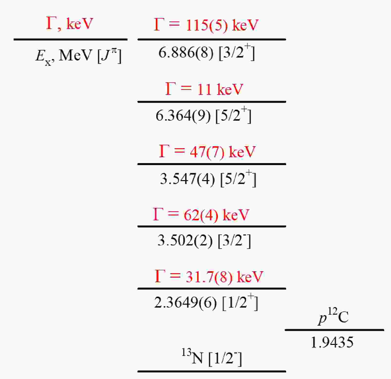
Now, we consider the spectrum of resonance levels and determine their role in the studied reaction ${^{12}}{\text{C}}{(p,{\gamma _0})^{13}}{\text{N}}$. The spectrum of the ¹³N levels at energies up to 5 MeV above the p¹²C channel threshold is shown in Figure 1.

Figure 1.  (color online) The energy spectrum of ¹³N in MeV [28]. The widths Γ of the levels in c.m. are marked in red.

The available experimental data on the astrophysical S-factor [13,14,26,27] show the presence of a narrow J^π = 1/2⁺ resonance with a width of about 32 keV at E_c.m. = 0.421 MeV or the excitation energy E_x = 2.3649(6) MeV. Presently, it can be considered precisely established that this resonance is due to the ²S_1/2-wave, and consequently, its excitation in S(E) factor is the signature of E1 transition to the ground ²Р_1/2 state of the ¹³N nucleus.

Another resonance taken into consideration corresponds to the J^π = 3/2^- state at the excitation energy E_x = 3.502 MeV (E_c.m. = 1.559 MeV). It is compared to the ²P_3/2-wave without FS.

All other resonances in Figure 1 do not lead to p,γ-channels and will not be studied [28] (see Table 13.14). However, we consider the ²D_3/2-wave with FS and quantum numbers J^π = 3/2⁺. Present calculations are limiting by E1 and M1 processes. That is why the states with the momentum of 5/2⁺ at E_x = 3.547 and 6.564 MeV compared to the ²D_5/2-wave, providing M2 transition, are out of consideration.

Thereby, we treated three partial transitions of proton radiative capture to the $ {}^2{P_{1/2}} $ GS of ¹³N. They are classified following the spectroscopic notation $ {\left[ {{}^{2S + 1}{L_J}} \right]_i}\xrightarrow{{NJ}}{}^2{P_{1/2}} $. These are two resonance transitions: $ {}^2{S_{1/2}}\xrightarrow{{E1}}{}^2{P_{1/2}} $ and $ {}^2{P_{3/2}}\xrightarrow{{M1}}{}^2{P_{1/2}} $, and non-resonance one $ {}^2{D_{3/2}}\xrightarrow{{E1}}{}^2{P_{1/2}} $.

Table 1 represents the results on the potential parameters of p+¹²C elastic scattering waves included in consideration of the astrophysical S-factor in Section 3.

The R-matrix fits of Refs. Kettner et al., 2023 [12] and Skowronski et al. [13,14] give the values: Γ_c.m.( 1/2⁺) = 31.4 ± 0.2 keV and 33.8 keV, Γ_c.m.(3/2^-) = 50.9 ± 0.3 keV and 54.2 keV, respectively. These parameters are comparable with MPCM ones.

Kelley et al., 2024, provide the most complete data on the ¹³N levels in a recent compilation [29]. One more may be added: Anh et al., 2024 reported the results of measurements on the 1/2⁺ and 3/2^- resonances. These are: E_res = 421 keV, Γ_c.m. = 34.1 keV, and E_res = 1554 keV, Γ_c.m. = 56.5, respectively [30].

Figure 2 shows the phase shifts of ²S_1/2, ²P_3/2, and ²D_3/2 partial waves calculated with the parameters of Table 1. Here and elsewhere, the scattering phase shifts at E_c.m. = 0 are determined based on the generalized Levinson theorem [31]

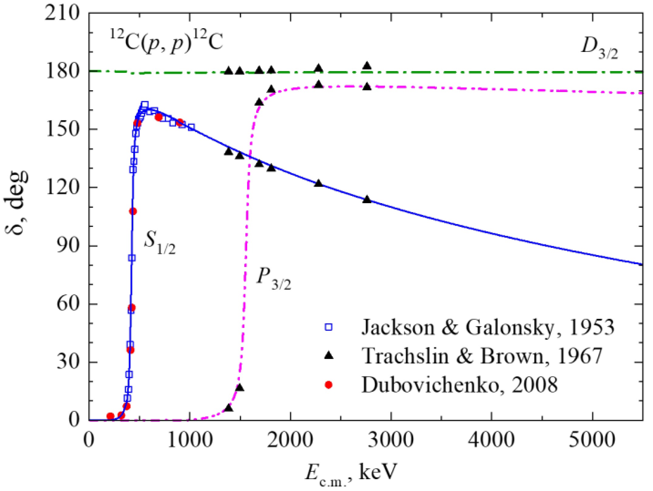
Figure 2.  (color online) Elastic p¹²С scattering phase shifts at low energies. The results of ²S_1/2 phase shift analysis: red dots from Ref. [32], Dubovichenko, 2008; the blue open squares are from Ref. [33], Jackson & Galonsky, 1953; the black solid triangles are from Ref. [34], Trachslin & Brown, 1967. The curves are calculated with potential parameters from Table 1.

No	Ex, exp.	$ J_i^\pi $, 2S+1LJ	Γc.m., exp.	Eres, exp.	V0	α	Eres, theory	Γc.m., theory
1	2.3649(6)	1/2+, 2S1/2	31.7(8)	0.4214(6)	101.486	0.195	0.422	32
2	3.502(2)	3/2-, 2P3/2	62(4)	1.559(2)	833.114	2.9	1.560	53
3	—	3/2+, 2D3/2	—	—	320.0	0.4	—	—
Note, the recent experimental data on the 1/2+ and 3/2- levels are reported by Csedreki et al., 2023: Eres = 424.2 ± 0.7 keV, Γc.m. = 35.2 ± 0.5 keV, and Eres = 1554.6 ± 0.6 keV, Γc.m. = 53.1 ± 0.7 keV, respectively [10]. Comparison with the recommended data by Ajzenberg-Selove, 1991, [28] shows the most difference of the 3/2- level widths. Therefore, while fitting the corresponding potential parameters of 2P3/2 resonance wave, we oriented on the Ref. [10].

Table 1.  Characteristics of the continuous spectrum states in the p¹²C channel. Excitation and resonance energies E_x and E_res are provided in MeV, and the level widths Γ_c.m. are in keV. $ J_i^\pi $ is the total angular momentum and parity of the initial state. Parameters of interaction potential (1) are V₀ in MeV and α in fm^-2. Experimental data are from Ref. [28]

where N_L and M_L are the numbers of forbidden and allowed bound states, respectively, and L is the orbital angular momentum. According to this theorem, the phase shifts are positive and tend to zero at high energies. The ²D_3/2 potential with FS leads to the phase shift of 180(1)°. The S-wave phase shift should be δ_S(0) = 180° according to Levinson theorem (2). In Figure 2 it starts from zero in order to confine all curves within a uniform range of values.

The comparison of the calculated phase shifts $ {\delta _{^2{S_{1/2}}}} $, $ {\delta _{^2{P_{3/2}}}} $, and $ {\delta _{^2{D_{3/2}}}} $ with the experimental data of Refs. [32–34] shows very good agreement in the energy region up to E_c.m. = 3 MeV. The independent checkup of MPCM results is available for the resonance phase shifts $ {\delta _{^2{S_{1/2}}}} $, $ {\delta _{^2{P_{3/2}}}} $calculated using the multilevel, multichannel R-matrix code, AZURE – Figure 1 in Ref. [35]. The cross-confirmation of the energy dependence of the $ {\delta _{^2{S_{1/2}}}} $ and $ {\delta _{^2{P_{3/2}}}} $ phase shifts is provided by the calculations in the framework of cluster effective field theory (CEFT) in Figure 6 of early Ref. [36]. The results of CEFT may be assumed as an additional confirmation for the MPCM approach.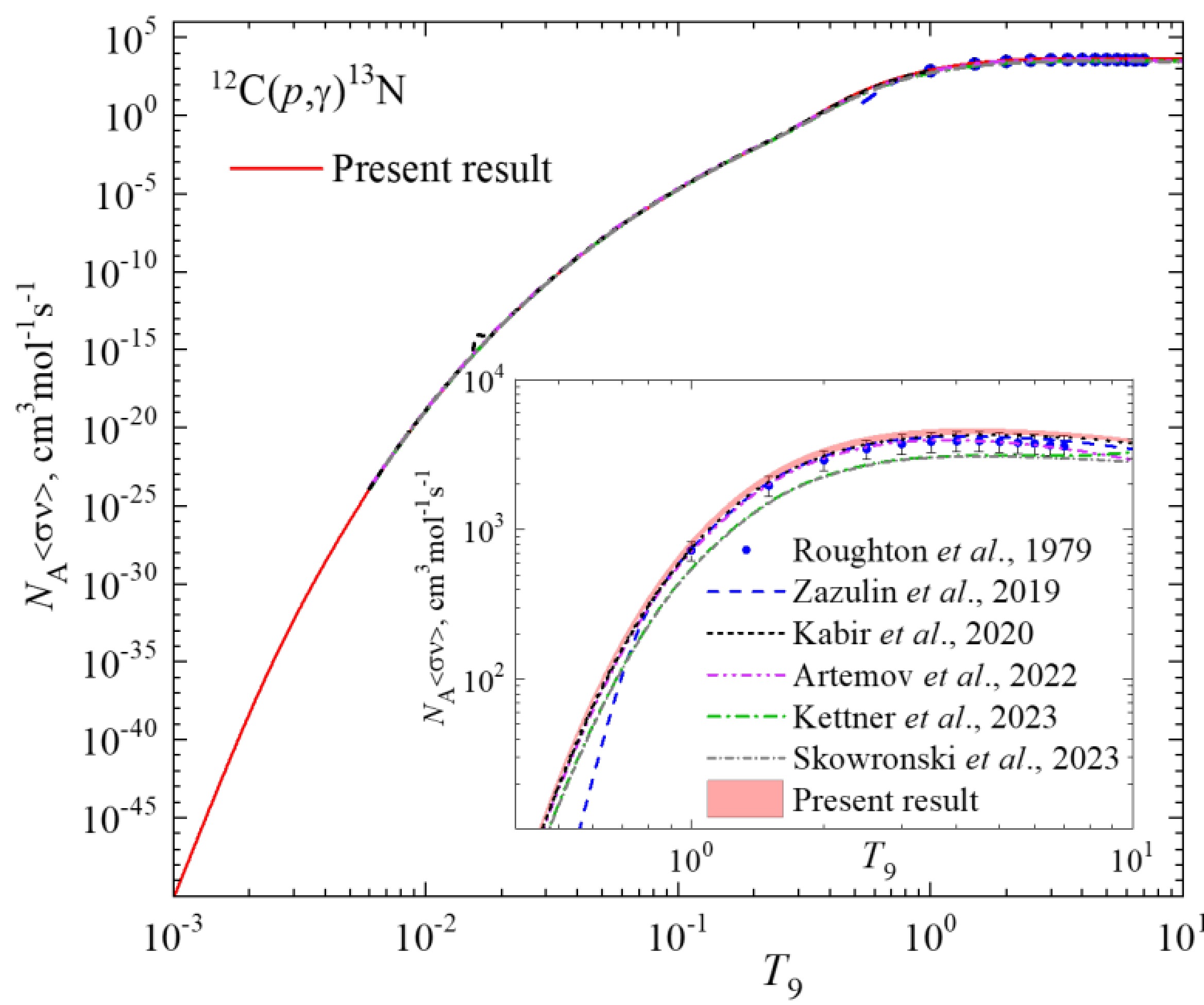

Figure 6.  (color online) The p¹²C capture reaction rate. The blue dots are from work [62], the blue dashed curve from [47], the black short-dashed curve from Ref. [61], the purple dash-double-dotted curve from Ref. [43], green the dash-dotted curve from Ref. [12], the grey short-dash-dotted curve from Ref. [13], and the red solid curve is the present MPCM results. The inset shows the interval of T₉ = 0.4 – 10.

The bound state potential construction is conditioned by independent information on the asymptotic normalization coefficients (ANC) in the single cluster channel. The ANC is related to the dimensional asymptotic constant C via the spectroscopic factor S_f ${A_{NC}} = \sqrt {{S_f}} \cdot C$ [37].

We use the dimensionless asymptotic constant C_w introduced in Ref. [38] which is related to the dimensional $ C=\sqrt{2{k}_{0}}\cdot {C}_{w} $. Therefore, the following expression holds: ${C_w} = \frac{{{A_{NC}}}}{{\sqrt {{S_f}} \cdot \sqrt {2{k_0}} }}$. Wave number ${k_0}$ is related to the binding energy ${E_b} = k_0^2{\hbar ^2}/2\mu $ and$\sqrt {2{k_0}} = 0.768$ fm^-1/2 for the p¹²C system. Table 2 gives the known values of ANC and their recalculation to dimensionless asymptotic constant C_w.

For the value of the spectroscopic factor S_f, we utilized the data provided in Table 2 from Ref. [41]. The data from 18 studies have been analyzed in [41], focusing on stripping and pickup reactions on ¹²C target with projectiles d, ³He, α, ⁷Li, ¹⁰B, ¹⁴N, ¹⁶O within the time range of 1967 to 2010. The averaged interval of values for the spectroscopic factor is S_f = 0.87(62).

The potential parameters for the GS of ¹³N are adjusted in such a way as to reproduce the channel binding energy and experimental data for the mean charge radius with a given accuracy. In the р¹²С channel E_b = 1.9435 MeV [28]. For the charge radius data, Ref. [44] gives R_ch(¹³N) = 2.45(4) fm, and the most recent 2024-year work reports the value R_ch(¹³N) = 2.37(16) fm [45].

In Table 3, we present two sets of potential parameters that differ in asymptotic constant С_w values, but both reproduce the binding energy E_b with 10^-5 accuracy and give charge radius of $ {R_{{\text{ch}}}}{(^{13}}N) = 2.465 \pm 0.05\,\,{\text{fm}} $, which is within the interval of experimental values [44,45].

Let us comment the computing procedure providing the calculation of radial matrix elements of EJ-transitions $ {I_{{\text{E}}J}}(k,{J_f},{J_i}) = \left\langle {{\chi _f}} \right|{r^J}\left| {{\chi _i}} \right\rangle $ and MJ-transitions $ {I_{{\text{M}}J}}(k,{J_f},{J_i}) = \left\langle {{\chi _f}} \right|{r^{J - 1}}\left| {{\chi _i}} \right\rangle $ (the formalism details see in [24]). Overlapping integrals are calculated up to 50 fm. The initial scattering radial WF $ {\chi _i}(r) $is normalized to the asymptotics at the edge of the 50 fm interval, denoted as R

where F_L and G_L are the regular and irregular Coulomb functions, $ \delta _{S,L}^J $ are the scattering phase shifts. Relation (3) provides the calculation of phase shifts at two matching points [20].

The final radial WF $ {\chi _f}(r) $ for the bound states are the numerical ones on the interval r = 0–12 fm, as at larger distances the function reaches stable asymptotic behavior [38]

where ${W_{ - \eta \,\,L + 1/2}}(2{k_0}r)$is the Whittaker function. The difference between the AC values at the beginning of the stabilization region, starting from R = 12 fm, usually does not exceed 10^-3 – 10^-4 – this value is specified as the relative accuracy of determining the AC.

Figure 3 shows the radial dependence of the ²P_1/2 GS wave function, scattering S-wave function calculated at E_c.m. = 5 MeV and integrand I(r) corresponding to E1 matrix element $ {I_{{\text{E1}}}}(k,{J_f},{J_i}) = \left\langle {{\chi _f}} \right|{r^{}}\left| {{\chi _i}} \right\rangle $. One can see the internal node in ${\chi _i}$ wave due to the FS according to the above symmetry classification, contrary to the nodeless ${\chi _f}$ bound state function. Thereby, we illustrated the peripheral character of the ${^{12}}{\text{C}}{(p,{\gamma _0})^{13}}{\text{N}}$process, i.e., the integral ${I_{E1}}(k,{J_f},{J_i})$ accumulates in the interval r ~ 5-10 fm at E_c.m. = 5 MeV. We tried to employ the shallow phase-equivalent potentials for the S-wave [24], but they led to the completely inappropriate description of the first 1/2⁺ resonance at 0.421 MeV in the S-factor, i.e., overestimation of 2-3 orders of magnitude.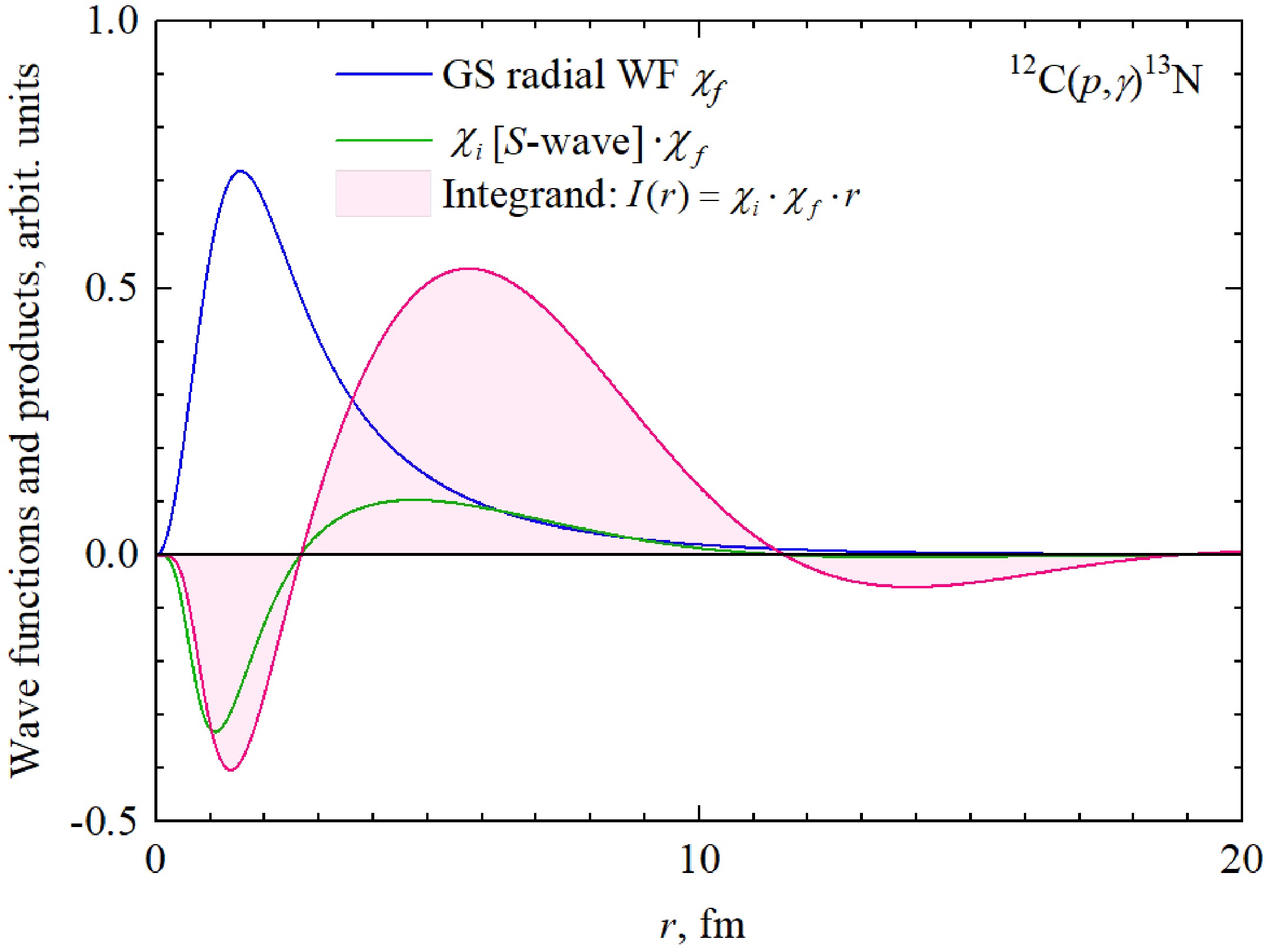

Figure 3.  (color online) The ground state WF of the ¹³N nucleus in the p¹²C channel (blue curve, Set I in Table 3); product of the ground state WF and scattering S-wave function calculated at E_c.m. = 5 MeV (green curve, Table 1); I(r) is integrand corresponding to E1-transition (filled area).

The results of MPCM calculations of the astrophysical S-factor in the energy interval from 25 keV to 5 MeV are shown in Figure 4. The magenta band is the total S-factor and refers to the interval of the asymptotic constant $1.30 \leqslant {C_w} \leqslant 1.37$. The low and upper bounding band curves refer to Set I and Set II for the GS potential from Table 3, respectively.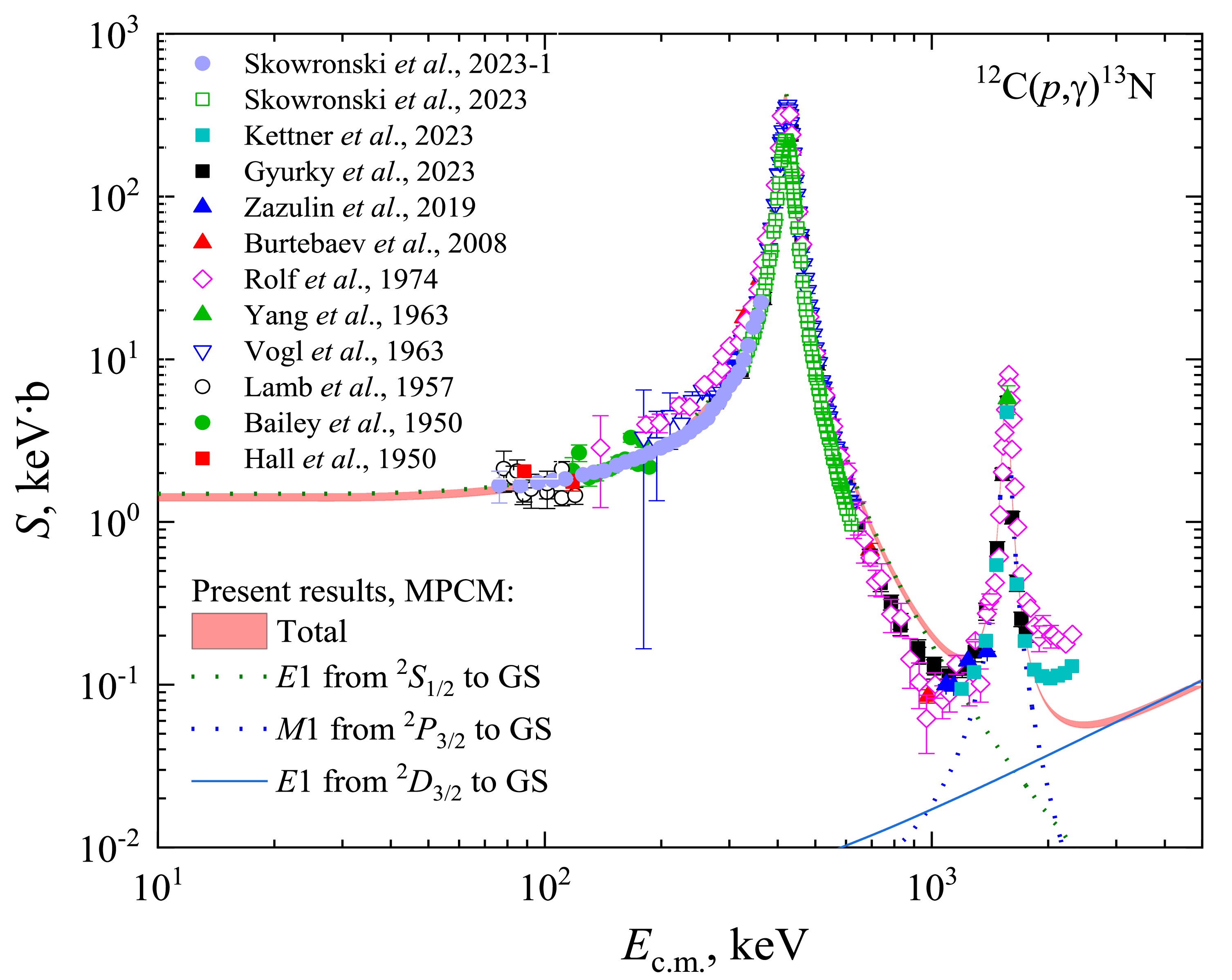

Figure 4.  (color online) Astrophysical S-factor of the radiative р¹²С capture at low energies. The experimental data are designated and taken from works [11–14,26,27,46–51]. The curves represent calculations with potentials from Tables 1 and 3.

The partial structure of the S-factor is determined well enough. The resonances 1/2^- and 3/2⁺ reveal at E_c.m. = 0.421 MeV and E_c.m. = 1.559 MeV, respectively. The 1^st resonance is determined by $ {}^2{S_{1/2}}\xrightarrow{{E1}}{}^2{P_{1/2}} $ transition and a tail of the 2^nd resonance due to $ {}^2{P_{3/2}}\xrightarrow{{M1}}{}^2{P_{1/2}} $ partial transition. The energy dependence of the S-factor above 2 MeV is provided predominantly by the non-resonance $ {}^2{D_{3/2}}\xrightarrow{{E1}}{}^2{P_{1/2}} $ transition. The S-factor error of ~ 1-2% is determined by the error of numerical methods.

The comparison of the calculated S-factor and experimental data in Figure 4 shows good agreement in general, but there are some deviations. In the interval E_c.m. ~ 640 – 930 keV, the average overestimation factor is ~ 1.3-1.5. On the right of the minimum in the region of the 2^nd resonance, i.e., E_c.m. ~ 1200 – 1850 keV theory is in very good agreement with experimental points of Gyürky et al., 2023 [11] and Kettner et al., 2023 [12]. However, experimental points at E_c.m. > 2000 keV from Refs. [26] and [12] are higher than the MPCM curves.

We cannot explain the origin of these differences since both the experimental data on the scattering phase shifts in Figure 2 and the parameters of the resonance levels (Table 1) are reproduced with high accuracy. However, these deviations do not affect the value of the S(E)-factor at low energies relevant to the astrophysical applications.

Note that some other model calculations of the S-factor meet the analogous problems with reproducing the right slope of the 1^st resonance [52–55].

Let us now turn to the discussion of the astrophysical S-factor at low energies relevant to the stellar temperature conditions. To implement the extrapolation of the astrophysical S-factor to the low energies, we use the well-known expression for S-factor parametrization (see, for example, Ref. [56])

The interpolation procedure of our results was done in the range of 25–100 keV with an average χ² = 0.001. The parameters of expression (5) are given in Table 4.

The summary of the astrophysical S-factors at 25 keV and S(0) discussed in literature since 1960 up to today is compiled in Table 5.

We would like to concentrate on the discussion of present low-energy results for Sets I and II with Luna data [14] and results reported by Kettner et al., 2023 [12]. As follows from Table 5 Set I leads to the astrophysical factor S(25) = 1.34 ± 0.02 keV·b, which is in excellent agreement with data by Skowronski et al., 2023 – 1.34 ± 0.09 keV·b [14]. While MPCM calculations with Set II give S(25) = 1.49 ± 0.02 keV·b, which is in excellent agreement with data by Kettner et al., 2023 – 1.48 ± 0.09 keV·b [12]. The difference between these two data sets is ~ 9-11 % at 25 keV.

Somewhat another conformity follows from the data given in work [9]: astrophysical S-factor S(E) in the range of 5-140 keV in the first row in Table 6 are taken from SF III [9] (see Table XI) and referred as Skowronski et al. [14], % uncertainty is pointed in brackets. Comparison with present MPCM calculations shows very good agreement with results obtained with Set II for the potential parameters of Table 3. We believe that comments on some of these differences should be addressed to the authors of [9]. The analysis of the causes is beyond our competence.

In Figure 5 we illustrate the quality of reproducing the LUNA data [14] for the astrophysical S-factor and in the framework of MPCM – the experimental points within the error bars are laying in the calculated band.

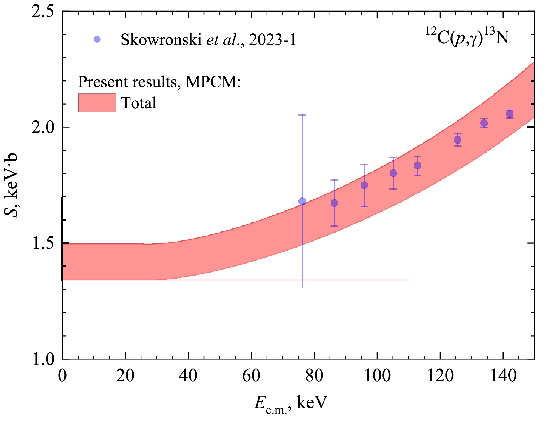
Figure 5.  (color online) Comparison of MPCM astrophysical S-factor and LUNA data [14]. The band refers to Sets I and II in Table 3.

The reaction rate of the radiative capture of protons (p,γ) with an equilibrium velocity distribution in the stellar environment is calculated as an integral of the total cross section weighted by the Maxwell-Boltzmann factor [4]

where N_A is the Avogadro number, µ is the reduced mass of two interacting particles, k_B is the Boltzmann constant, T is the temperature of the stellar environment.

Specifying the numerical constants in (6) and measurement units, one obtains the reaction rate in cm³mol^-1s^-1

for Т₉ in 10⁹ К, Е in MeV, the cross section $ \sigma (E) $in μb, μ in amu.

The total cross sections $ \sigma (E) $ in the range of E_c.m. from 1 keV to 5 MeV are used for the calculation of the reaction rate. To provide the cross sections at ultra-low energy, we use the well-known relation $S(E) = \sigma (E)E{e^{2\pi \eta }}$. Numerical calculation of the S-factor is performed from 25 keV to 5 MeV, and at lower energy, its value for 25 keV is used. In the energy range of 1 – 25 keV, the S-factor enters the stabilization region, which follows from the approximation (5) with parameters from Table 4 and illustrated in Figure 5.

The results of the MPCM calculations of the reaction rate $ {N_A}\left\langle {\sigma v} \right\rangle $ in the range from T₉ = 0.001 to T₉ = 10 based on the astrophysical S-factor illustrated in Figure 4 are shown in Figure 6. As for the value of $ {N_A}\left\langle {\sigma v} \right\rangle $ varies near 50 orders of magnitude in the pointed T₉ interval the band corresponding to the two sets of S-factor is visible only in inset in Figure 6.

The difference between the current calculations and the available reaction rates is evident in the inset of Figure 6, where the disparity in absolute values is clearly visible. The ratios of the reaction rates to NACRE II [16], as depicted in Figure 7, reveal additional information.

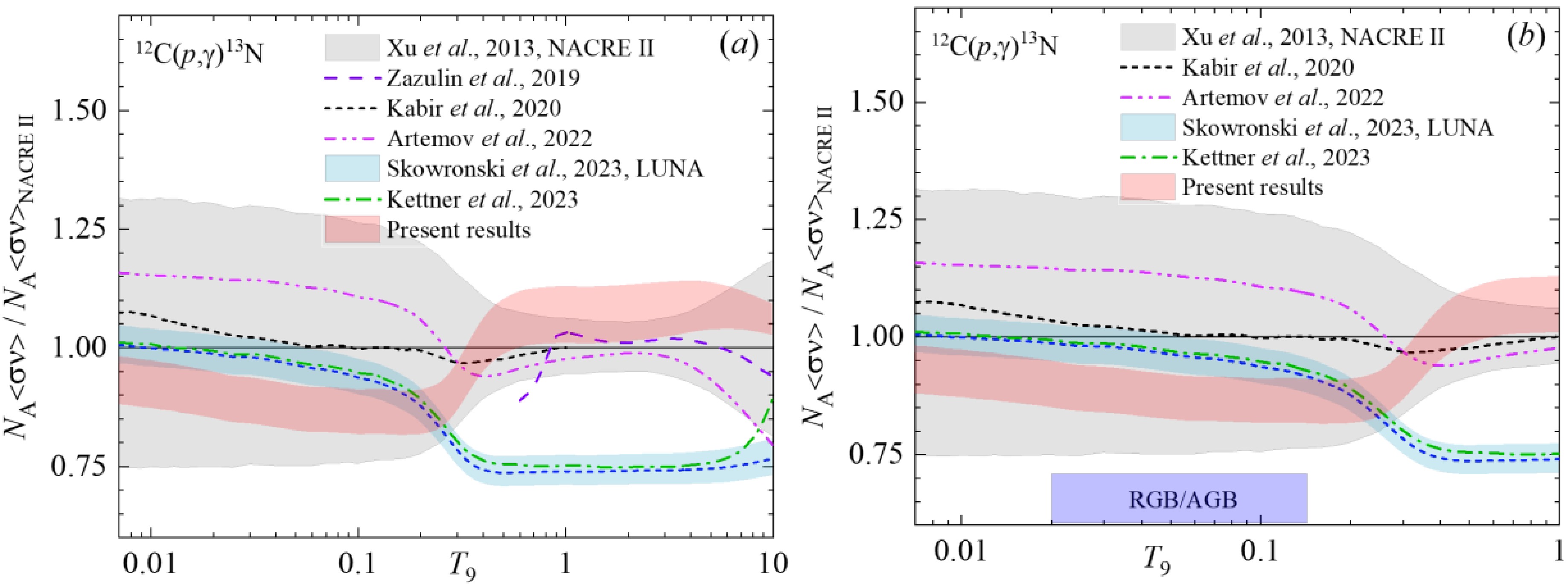
Figure 7.  (color online) Reaction rate ratio to NACRE II values for the ¹²C(p,γ)¹³N [16]: (a) the temperature range T₉ = 0.007 – 10; (b) the temperature range T₉ = 0.007 – 1. The violet bar indicates the temperature range of relevance for RGB and AGB stars. In both panels the central blue short-dashed curve in the band refers to the adopted reaction rate from [13,14].

Figure 7 shows the results of only the most recent publications [12,13,43,47,61]. The R-matrix procedure was exploited by Zazulin et al., 2019 [47], Artemov et al., 2022 [43], Kettner et al., 2023 [12]; and Skowronski et al., [13] for the calculation of S-factors and consequent reaction rates. The comparison of the rates in Figure 7 shows the difference in-between, as well as with the adopted NACRE II values. However, the rates by Zazulin et al., 2019 [47] and Artemov et al., 2022 [43] are within the gray band corresponding to the low and high NACRE II data.

Figure 7a shows near-precise reproducing of the adopted NACRE II reaction rate at T₉ = 0.006 - 1 by Kabir et al., 2020 [61]. This work uses the potential model for the calculation of the cross section in the energy range refers to the 1^st resonance, i.e. covers E_c.m. ≤ 1MeV.

Our focus is on the results of works of Kettner et al., 2023 [12]; Skowronski et al., 2023 [13,14]. As follows from Figure 7, the reaction rates obtained in these works as R-matrix best-fit procedure for the experimental S-factors are consistent throughout the entire temperature range less than 2% except the temperatures 6 ≤ Т₉ ≤ 10 where the difference reaches 2.4 – 16.6%. The ~ 5% deviation from NACRE II appears at Т₉ $\simeq $ 0.1 and reaches ~ 25% at higher Т₉. Present reaction rate comparing the adopted NACRE II is ~ 10 % lower at Т₉ < 0.2, but becomes higher than NACRE II near 5-15% starting from Т₉ $\simeq $ 0.4 and up to Т₉ = 10.

Figure 8 illuminates the range of deviation of the current MPCM reaction rate and those of the R-matrix fit of Refs. [12] and [14]. Skowronski et al., 2023 discuss in detail the ¹²C/¹³C evolution in AGB and RGB stellar environment in the T₉ = 0.02 – 0.14 range and propose the value of 3.6 ± 0.4 as the most precise up to now. Following [14] the carbon isotopic ratio is defined via the ¹²C and ¹³C densities ${n_{12}}$ and ${n_{13}}$ inversely proportional to the reaction rates: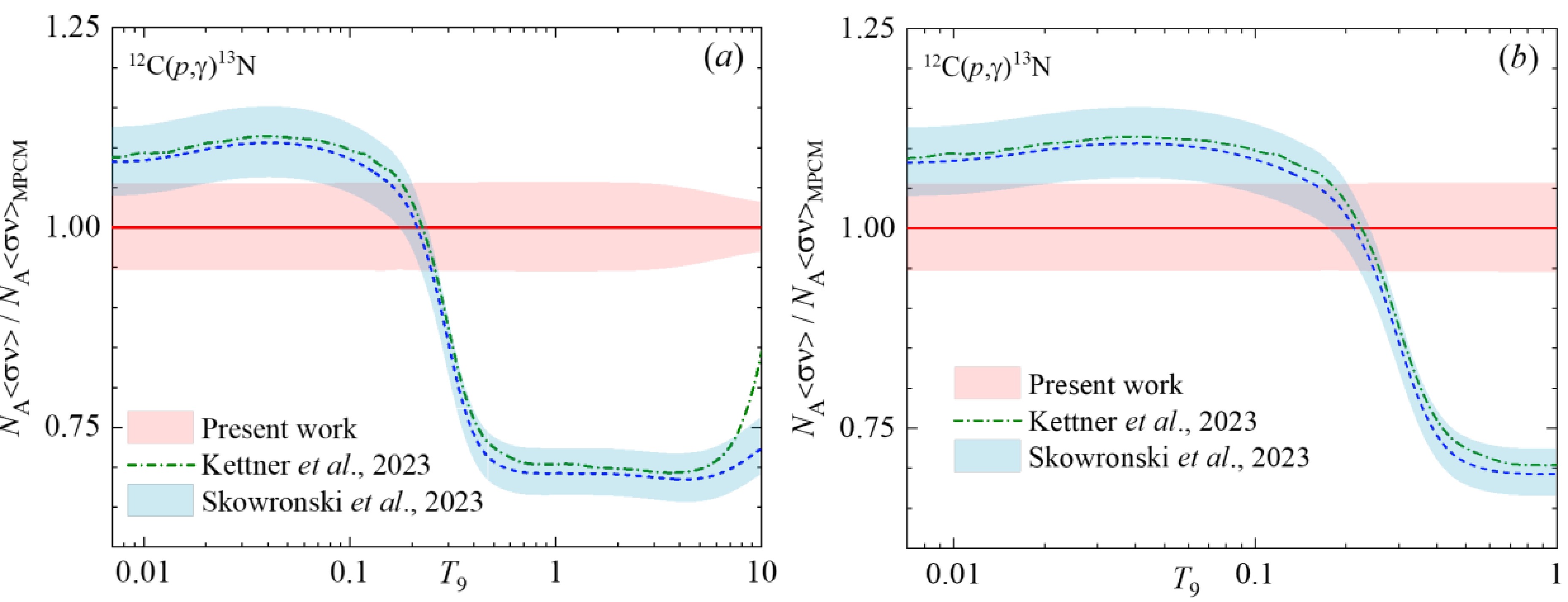

Figure 8.  (color online) Reaction rates of Kettner et al., 2023 [12] and Skowronski et al., [13,14] ratio to MPCM values for the ¹²C(p,γ)¹³N: (a) the temperature range T₉ = 0.007 – 10; (b) the temperature range T₉ = 0.007 – 1. In both panels the central blue short-dashed curve in the band refers to the adopted reaction rate from [13,14].

For reaction ¹²C(p,γ)¹³N in the temperature range T₉ from 0.02 to 0.14, the reaction rates ${\left\langle {\sigma v} \right\rangle _{12}}$vary from ${10^{ - 14}}$ cm³mol^-1s^-1 to 10^-4 cm³mol^-1s^-1that is, the difference is 10 orders of magnitude.

Even a small change in the numerical values of the rates may affect the calculated value of the ratio ¹²C/¹³C. It is most reliable to compare the reaction rates ¹²C(p,γ)¹³N and ¹³C(p,γ)¹⁴N obtained in the same formalism. So, for example, as it is done in the work of Skowronski et al., 2023, where the rates of these reactions are obtained in R-matrix calculations – this is a consistent approach. In this context, calculations of the reaction rate of ¹³C(p,γ)¹⁴N in MPCM and its comparison with those of ¹²C(p,γ)¹³N can make an additional contribution to the independent assessment of the ¹²C/¹³C ratio since the model errors are reduced.

In the present stage, we may compare the reaction rates for the processes ¹²B(n,γ)¹³B(βν)¹³C and ¹²C(p,γ₀)¹³N(β⁺)¹³C calculated in the MPCM – Figure 9. Both reactions are leading to the creation of carbon isotope ¹³C, but in the first case, the boron sequence is involved (see our works [15] and [63]) without combustion of ¹²C. The second chain refers to the hydrogen burning of ¹²C, therefore, the amount of ¹³C increases, while the abundance of ¹²C decreases.

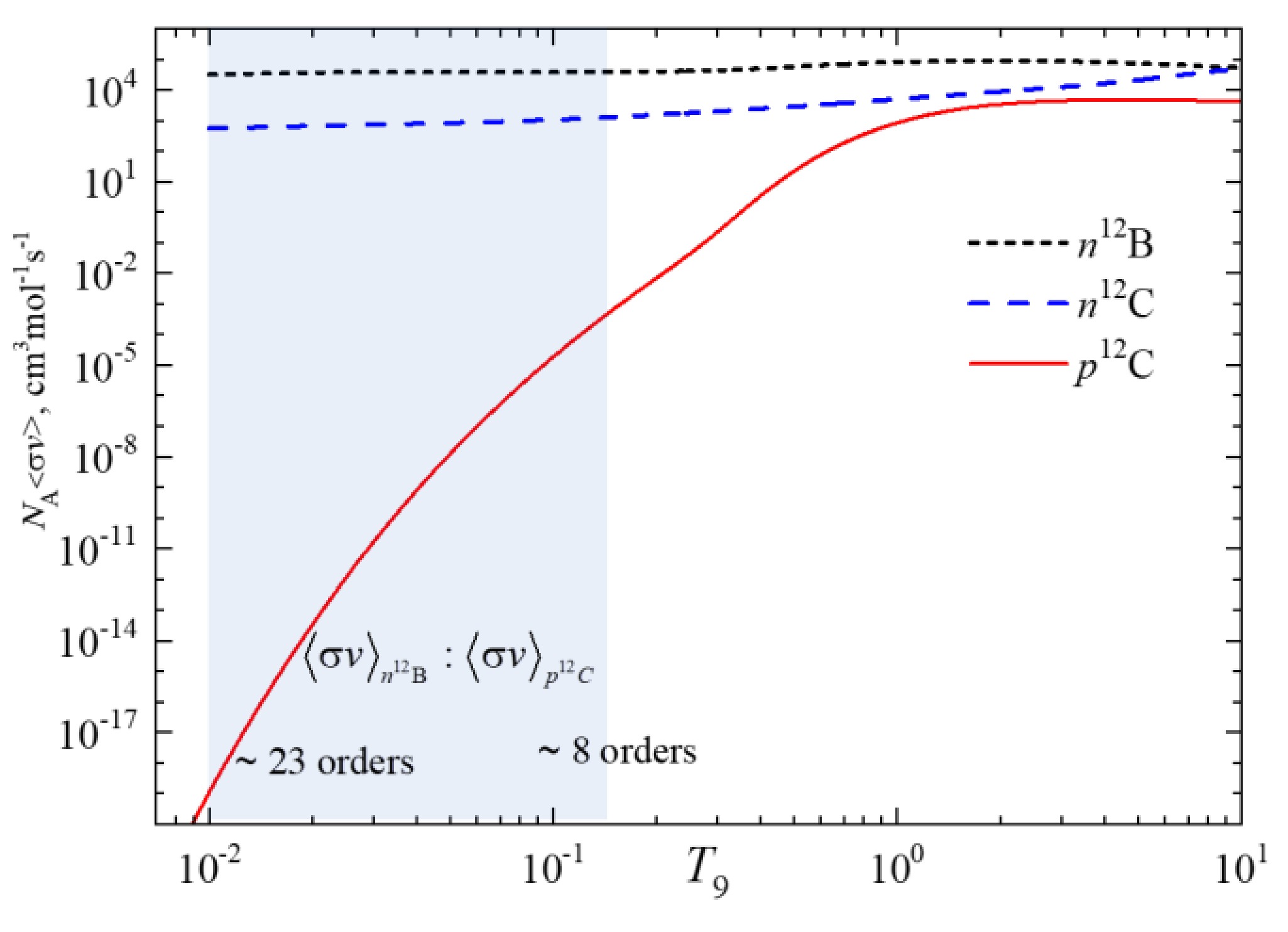
Figure 9.  (color online) Reaction rates calculated in MPCM: black dotted curve – ¹²B(n,γ₀)¹³B, dashed blue curve – ¹²C(n,_γ0+1+3+2)¹³C [15]; red solid curve – ${^{13}}{\text{C}}{(p,{\gamma _0})^{14}}{\text{N}}$, present work. The filled area refers to the interval of T₉ = 0.01 – 0.14.

To compare the reaction rates in Figure 9, the temperature range T₉ = 0.01 – 0.14 relevant for the post-BBN nucleosynthesis and stellar CNO cycles is highlighted in blue. The ratio of reaction rates $ {R_{{\text{B}}/{\text{C}}}} = \dfrac{{{{\left\langle {\sigma v} \right\rangle }_{{n^{12}}{\text{B}}}}}}{{{{\left\langle {\sigma v} \right\rangle }_{{p^{12}}{\text{C}}}}}} $ is of ~ 10²³ orders of magnitude at T₉ = 0.01, and ~ 10⁸ at T₉ = 0.14. One may assume that such a dominance of ¹²B(n,γ)¹³B(βν)¹³C chain over the rate of ¹²C(p,γ₀)¹³N(β⁺)¹³C path may change the initial composition of ¹²C and lead to the redistribution of ¹²C and ¹³C. It is expediently to estimate this correction for the ${R_{^{12}C{/^{13}}C}}$ ratio.

We have calculated the astrophysical S-factor for the proton radiative capture reaction ¹²C(p,γ)¹³N in the energy range of E_c.m. = 1 keV – 5000 keV. The reliability of MPCM current calculations is provided by the reproducing of the experimental phase shifts $ {\delta _{^2{S_{1/2}}}} $, $ {\delta _{^2{P_{3/2}}}} $, and $ {\delta _{^2{D_{3/2}}}} $at the energies up to E_c.m. = 3 MeV with high accuracy. Besides, the determined parameters of the 1/2⁺ and 3/2^- resonances, i.e. E_res = 422 keV, Γ_c.m. = 32 keV, and E_res = 1560 keV, Γ_c.m. = 53 keV, respectively, are in good agreement both with the recent experimental data by Csedreki et al., 2023, as well with R-matrix fit most recent results of Refs. [12–14,43].

The GS main characteristics, namely the binding energy in the p +¹²C channel E_b = 1.94350 MeV and charge radius $ {R_{{\text{ch}}}}{(^{13}}N) = 2.465 \pm 0.05\,\,{\text{fm}} $are calculated with 10^-5 MeV and 10^-2 fm accuracy, respectively. Two sets of potential parameters for the GS radial wave function have been found under the condition that E_b remains constant, but the values of the asymptotic constant C_w are different. Set I refers to C_w = 1.30(2), and Set II refers to C_w = 1.37(1).

Set I leads to the astrophysical factor S(25) = 1.34 ± 0.02 keV·b, which is in excellent agreement with data by Skowronski et al., 2023 – 1.34 ± 0.09 keV·b [14]. Set II gives S(25) = 1.49 ± 0.02 keV·b, which is in excellent agreement with data by Kettner et al., 2023 – 1.48 ± 0.09 keV·b [12]. The difference between these two data is ~ 9-11% at 25 keV. Therefore, we are able to reproduce both results for the S(0), which demonstrates the flexibility of MPCM formalism at a well-substantiated level.

One cannot but agree that the R-matrix approach is a fitting of experimental data, and it is difficult for model calculations to compete with it. The MPCM succeeded in reproducing the known today experimental data for the astrophysical S(E) factor in the energy range from 76 keV up to 2000 keV, but met the problem at the energies E_c.m. ~ 640 – 930 keV, refer to the "slope" of the 1^st (1/2⁺) resonance. Current calculations show a near 30 – 50% overestimation of the experimental S-factor within this energy range, and that has no explanation at the moment as the phase shifts $ {\delta _{^2{S_{1/2}}}} $, $ {\delta _{^2{P_{3/2}}}} $, and $ {\delta _{^2{D_{3/2}}}} $ providing the energy dependence of the calculated S-factor are reproduced precisely up to E_c.m. = 3 MeV as we stated above.

The reaction rate of the process ¹²C(p,γ)¹³N is calculated for the T₉ = 0.001 – 10. Typically, the NACRE II data are used as a benchmark for comparing subsequent calculations of the reaction rates. Figures 6 and 7 do not show neither qualitative nor quantitative exact agreement with the NACRE II data for all cited Refs. [12,13,43,47,61] and present work in the whole range of T₉ (may be some exception is Ref. [61], see comments above). However, there are temperature areas where acceptable agreement is observed for the reaction rates. R-matrix results for the reaction rate by Skowronski et al., 2023 [13] and Kettner et al., [12] show excellent agreement up to T₉ $\simeq $ 6 between themselves. However, there are also the R-matrix calculations, for example, [43] and [47] with very close input parameters, which yield noticeably different outcomes.

Finally, we may conclude that any of the known reaction rates of the ¹²C(p,γ)¹³N process may be recommended for the calculation of the astrophysical macro-characteristics like mass fraction or efficiency of ¹²C production if the deviations within the ~ 30-50 % are acceptable. Otherwise, the issue of ¹²C(p,γ)¹³N reaction rate consensus remains open.

While studying the ¹²C(p,γ)¹³N reaction, the results of MPCM approach show a reasonably reliable level; consequently, applying this model to the consideration of the ¹³C(p,γ)¹⁴N reaction is actual.

We approximate the reaction rates of Table A1 calculated in MPCM with the following expression:

The parameters a_i and b_i for two sets are provided in Table A2.

Calculation of ${\chi ^2}$ is implemented following the standard definition (see, e.g., [20])

where N is the number of the calculation points; $\left\langle {\sigma v} \right\rangle _i^{app.}({T_9})$ is approximated reaction rate Eq. (A1); $\left\langle {\sigma v} \right\rangle _i^{calc.}({T_9})$ is calculated reaction rate according to Eq. (7); the error $\Delta \left\langle {\sigma v} \right\rangle _i^{calc.}({T_9})$ we assume here to be 5% of the calculated reaction rate.