


 Abstract
 HTML
HTML Reference
 Related
 PDF
PDF


-
Generalized transverse momentum-dependent parton distributions (GTMDs) [1−3], which are often referred to as mother distributions, may be investigated to obtain a thorough understanding of hadron structure. As foundational distributions, GTMDs can be reduced to generalized parton distributions (GPDs) [4−18] and transverse momentum dependent parton distributions (TMDs) [19, 20] under specific limits. The GPDs and TMDs offer a comprehensive array of information related to the confined spatial distributions of quarks and gluons within bound hadrons. The GPDs represent the three-dimensional extension of conventional parton distribution functions (PDFs) [21−24] and are defined as the off-forward matrix elements associated with quark and gluon operators. Further, the GPDs are observables that encompass a wealth of previously inaccessible information regarding hadron structure. They are observed in exclusive processes such as deeply virtual Compton scattering (DVCS) [25] and timelike Compton scattering (TCS). A novel process known as double deeply virtual Compton scattering (DDVCS) was recently introduced [14, 26]. In contrast to DVCS, DDVCS involves an electron scattering off a nucleon, which produces a lepton pair. A notable feature of DDVCS is its potential for the direct measurement of GPDs at
$ x \neq \pm \xi $ at the leading order. When quantum chromodynamics (QCD) factorization is applicable, the amplitude of high-energy processes can be expressed as a convolution of a hard perturbative kernel and GPDs. The GPDs provide more comprehensive information than PDFs and form factors (FFs) [27−29] related to the internal structure of hadrons. For example, they encapsulate insights into spin contributions from quarks and gluons within nucleons, as demonstrated in Refs. [5, 30]. Consequently, GPDs serve as valuable tools to clarify the transverse spatial distribution of partons.Extensive research on GPDs has been conducted given their significance in understanding hadronic structure dynamics, and comprehensive results have been presented in reviews [8, 31, 32]. However, measuring GPDs experimentally remains challenging. Consequently, first-principles computations using lattice (QCD) have focused on their lowest Mellin moments. Therefore, enhancing our theoretical understanding of GPD behavior can facilitate more accurate experimental determinations.
The Sullivan process [33] considers the off-shell characteristics of the GPDs of pions. The presence of off-shellness disrupts crossing symmetry, which leads to the emergence of new off-shell FFs. In this study, we investigate the off-shell GPDs and examine the relationship between these off-shell gravitational FFs of pions [34].
Investigation into the transverse momentum distribution of hadrons produced in semi-inclusive deep inelastic scattering (SIDIS) [35−37] is characterized by determining TMDs, which have been extensively studied [38−42]. In this paper, we also evaluate off-shell pion TMDs.
Pions are Nambu-Goldstone bosons associated with the chiral symmetry breaking in QCD among all hadrons, and they are believed to play a crucial role in the origin of mass and matter [43, 44]. Therefore, understanding how quarks and gluons combine to form pions is of paramount importance, and thus, gaining experimental insights into their structure would be highly valuable. Given its connection to chiral symmetry breaking, investigating the GPDs of pions is considered particularly significant.
In this study, we calculate the off-shell GPDs of pions within the framework of the Nambu-Jona-Lasinio (NJL) model [45−53]. The NJL model is a well-established phenomenological approach to quark matter that incorporates essential QCD features such as chiral phase transitions along with various interaction terms that describe both quark dynamics and their interactions. This model can accurately predict meson masses and decay constants while also playing a vital role in characterizing other properties of quark matter. Previous studies have already examined on-shell GPDs [9, 10, 12, 54−60], which allow us to compare our findings on off-shell GPDs effectively.
This remainder of this paper is organized as follows: In Sec. II, we begin with a concise introduction to the NJL model. Subsequently, we outline the process for defining and calculating pion off-shell GPDs. In Sec. III, we examine and discuss the fundamental properties of off-shell GPDs, with particular emphasis on FFs associated with these distributions. In Sec. IV, we explore the off-shell TMDs of pions. Finally, a brief summary and discussion are presented in Sec. V.
-
For a thorough understanding of hadron structure, one may investigate generalized transverse momentum-dependent parton distributions (GTMDs) [1−3], which are often referred to as the mother distributions. As the foundational distributions, GTMDs can be reduced to GPDs [4−18] and TMDs [19, 20] under specific limits. GPDs and TMDs offer a comprehensive array of information regarding the confined spatial distributions of quarks and gluons within bound hadrons. GPDs, which represent the three-dimensional extension of conventional parton distribution functions (PDFs) [21−24], are defined as the off-forward matrix elements associated with quark and gluon operators. GPDs are observables that encompass a wealth of previously inaccessible information regarding hadron structure. They arise in exclusive processes such as deeply virtual Compton scattering (DVCS) [25] and timelike Compton scattering (TCS). Recently, a novel process known as double deeply virtual Compton scattering (DDVCS) has been introduced [14, 26]. In contrast to DVCS, the DDVCS process involves an electron scattering off a nucleon, resulting in the production of a lepton pair. A notable feature of DDVCS is its potential for direct measurement of GPDs at
$ x \neq \pm \xi $ at leading order. When QCD factorization is applicable, the amplitude of high-energy processes can be expressed as a convolution of a hard perturbative kernel and GPDs. GPDs provide more comprehensive information than PDFs and form factors (FFs) [27−29] regarding the internal structure of hadrons. For instance, they encapsulate insights into the spin contributions from quarks and gluons within nucleons, as demonstrated in Refs. [5, 30]. Consequently, GPDs serve as valuable tools for elucidating the transverse spatial distribution of partons.Given their significance in understanding hadronic structure dynamics, extensive research on GPDs has been conducted; comprehensive results can be found in reviews [8, 31, 32]. However, measuring GPDs experimentally remains challenging; consequently, first-principles computations using lattice quantum chromodynamics (QCD) have primarily focused on their lowest Mellin moments. Therefore, enhancing our theoretical understanding of GPD behavior would facilitate more accurate experimental determinations.
In the Sullivan process [33], the off-shell characteristics of the GPDs of pions are taken into account. The presence of off-shellness disrupts crossing symmetry, leading to the emergence of new off-shell FFs. In this study, we will investigate the off-shell GPDs and examine the relationship between these off-shell gravitational form factors of pions [34].
The investigation into the transverse momentum distribution of hadrons produced in semi-inclusive deep inelastic scattering (SIDIS) [35−37] is characterized by determining TMDs. TMDs have been extensively studied [38−42]. In this paper, we will also evaluate off-shell pion TMDs.
Pions are Nambu-Goldstone bosons associated with the chiral symmetry breaking in QCD among all hadrons, and they are believed to play a crucial role in the origin of mass and matter [43, 44]. Therefore, understanding how quarks and gluons combine to form pions is of paramount importance; thus, gaining experimental insights into their structure would be highly valuable. Given its connection to chiral symmetry breaking, investigating the GPDs of pions is particularly significant.
In this study, we will calculate the off-shell GPDs of pions within the framework of the Nambu-Jona-Lasinio (NJL) model [45−53]. The NJL model is a well-established phenomenological approach to quark matter that incorporates essential QCD features such as chiral phase transitions along with various interaction terms that describe both quark dynamics and their interactions. It can accurately predict meson masses and decay constants while also playing a vital role in characterizing other properties of quark matter. Previous studies have already examined on-shell GPDs [9, 10, 12, 54−60], which will allow us to compare our findings on off-shell GPDs effectively.
This paper is structured as follows: In Sec. II, we begin with a concise introduction to the NJL model. Subsequently, we outline the process for defining and calculating pion off-shell GPDs. In Sec. III, we examine and discuss the fundamental properties of off-shell GPDs, with particular emphasis on the FFs associated with these distributions. In Sec. IV, we explore the off-shell TMDs of pions. Finally, a brief summary and discussion are presented in Sec. V.
-
Generalized transverse momentum-dependent parton distributions (GTMDs) [1−3], which are often referred to as mother distributions, may be investigated to obtain a thorough understanding of hadron structure. As foundational distributions, GTMDs can be reduced to generalized parton distributions (GPDs) [4−18] and transverse momentum dependent parton distributions (TMDs) [19, 20] under specific limits. The GPDs and TMDs offer a comprehensive array of information related to the confined spatial distributions of quarks and gluons within bound hadrons. The GPDs represent the three-dimensional extension of conventional parton distribution functions (PDFs) [21−24] and are defined as the off-forward matrix elements associated with quark and gluon operators. Further, the GPDs are observables that encompass a wealth of previously inaccessible information regarding hadron structure. They are observed in exclusive processes such as deeply virtual Compton scattering (DVCS) [25] and timelike Compton scattering (TCS). A novel process known as double deeply virtual Compton scattering (DDVCS) was recently introduced [14, 26]. In contrast to DVCS, DDVCS involves an electron scattering off a nucleon, which produces a lepton pair. A notable feature of DDVCS is its potential for the direct measurement of GPDs at
$ x \neq \pm \xi $ at the leading order. When quantum chromodynamics (QCD) factorization is applicable, the amplitude of high-energy processes can be expressed as a convolution of a hard perturbative kernel and GPDs. The GPDs provide more comprehensive information than PDFs and form factors (FFs) [27−29] related to the internal structure of hadrons. For example, they encapsulate insights into spin contributions from quarks and gluons within nucleons, as demonstrated in Refs. [5, 30]. Consequently, GPDs serve as valuable tools to clarify the transverse spatial distribution of partons.Extensive research on GPDs has been conducted given their significance in understanding hadronic structure dynamics, and comprehensive results have been presented in reviews [8, 31, 32]. However, measuring GPDs experimentally remains challenging. Consequently, first-principles computations using lattice (QCD) have focused on their lowest Mellin moments. Therefore, enhancing our theoretical understanding of GPD behavior can facilitate more accurate experimental determinations.
The Sullivan process [33] considers the off-shell characteristics of the GPDs of pions. The presence of off-shellness disrupts crossing symmetry, which leads to the emergence of new off-shell FFs. In this study, we investigate the off-shell GPDs and examine the relationship between these off-shell gravitational FFs of pions [34].
Investigation into the transverse momentum distribution of hadrons produced in semi-inclusive deep inelastic scattering (SIDIS) [35−37] is characterized by determining TMDs, which have been extensively studied [38−42]. In this paper, we also evaluate off-shell pion TMDs.
Pions are Nambu-Goldstone bosons associated with the chiral symmetry breaking in QCD among all hadrons, and they are believed to play a crucial role in the origin of mass and matter [43, 44]. Therefore, understanding how quarks and gluons combine to form pions is of paramount importance, and thus, gaining experimental insights into their structure would be highly valuable. Given its connection to chiral symmetry breaking, investigating the GPDs of pions is considered particularly significant.
In this study, we calculate the off-shell GPDs of pions within the framework of the Nambu-Jona-Lasinio (NJL) model [45−53]. The NJL model is a well-established phenomenological approach to quark matter that incorporates essential QCD features such as chiral phase transitions along with various interaction terms that describe both quark dynamics and their interactions. This model can accurately predict meson masses and decay constants while also playing a vital role in characterizing other properties of quark matter. Previous studies have already examined on-shell GPDs [9, 10, 12, 54−60], which allow us to compare our findings on off-shell GPDs effectively.
This remainder of this paper is organized as follows: In Sec. II, we begin with a concise introduction to the NJL model. Subsequently, we outline the process for defining and calculating pion off-shell GPDs. In Sec. III, we examine and discuss the fundamental properties of off-shell GPDs, with particular emphasis on FFs associated with these distributions. In Sec. IV, we explore the off-shell TMDs of pions. Finally, a brief summary and discussion are presented in Sec. V.
-
The off-shell GPDs of pions are examined within the framework of the spectral quark model (SQM) in the chiral limit, as discussed in Refs. [61, 62]. In this section, we calculate off-shell GPDs using the NJL model, and we compare our findings with the on-shell pion GPDs presented in Refs. [10, 12].
-
The SU(2) flavor NJL Lagrangian,
$ \begin{aligned}[b] {\cal{L}}=\;&\bar{\psi }\left(i\gamma ^{\mu }\partial _{\mu }-\hat{m}\right)\psi+\frac{1}{2} G_{\pi }\left[\left(\bar{\psi }\psi\right)^2-\left( \bar{\psi }\gamma _5 \vec{\tau }\psi \right)^2\right]\\ &-\frac{1}{2}G_{\omega}\left(\bar{\psi }\gamma _{\mu}\psi\right)^2-\frac{1}{2}G_{\rho}\left[\left(\bar{\psi }\gamma _{\mu} \vec{\tau } \psi\right)^2+\left( \bar{\psi }\gamma _{\mu}\gamma _5 \vec{\tau } \psi \right)^2\right], \end{aligned} $
(1) The expression
$ \hat{m}\equiv{\rm{diag}}\left[m_u,m_d\right] $ denotes the current quark mass matrix. Under the assumption of isospin symmetry, we have$ m_u = m_d = m $ . The symbols$ \vec{\tau} $ represent the Pauli matrices associated with isospin, while$ G_{\pi} $ ,$ G_{\omega} $ , and$ G_{\rho} $ refer to the four-fermion coupling constant in each chiral channel.The interaction kernel between elementary quarks and antiquarks is defined as follows:
$ \begin{aligned}[b] {\cal{K}}_{\alpha\beta,\gamma\delta}=\;&\sum\limits_{\Omega}K_{\Omega}\Omega_{\alpha\beta}\bar{\Omega}_{\gamma\delta} = 2iG_{\pi}[(1)_{\alpha\beta}(1)_{\gamma\delta}\\ &- (\gamma_5\tau_i)_{\alpha\beta}({\gamma_5\tau_i})_{\gamma\delta}]-2iG_{\rho}[(\gamma_{\mu}\tau_i)_{\alpha\beta}(\gamma_{\mu}\tau_i)_{\gamma\delta}\\& + (\gamma_{\mu}\gamma_5\tau_i)_{\alpha\beta}(\gamma_{\mu}\gamma_5\tau_i)_{\gamma\delta}]-2iG_{\omega}(\gamma_{\mu})_{\alpha\beta}(\gamma_{\mu})_{\gamma\delta}, \end{aligned} $
(2) where the indices denote Dirac, color, and isospin labels.
The dressed quark propagator in the NJL model is derived by solving the gap equation,
$ iS^{-1}(k)=iS_0^{-1}(k)-\sum\limits_{\Omega}K_{\Omega}\Omega \int \frac{d^4l}{(2\pi)^4}{\rm{tr}}[\bar{\Omega}i S(l)], $
(3) where
$ S_0^{-1}(k)={\not k}-m+i \varepsilon $ represents the bare quark propagator, and the trace is taken over Dirac, color, and isospin indices. The solution of gap equation is defined as$ S(k)=\frac{1}{\not k-M+i \varepsilon} . $
(4) The interaction kernel of the gap equation is local; therefore, we derive a constant dressed quark mass
$ M=m+12 i G_{\pi}\int \frac{d^4l}{(2 \pi )^4}{\rm{tr}}_{{\rm{D}}}[S(l)], $
(5) where the trace is taken over Dirac indices. Dynamical chiral symmetry breaking can occur only when the coupling strength exceeds a critical threshold, specifically
$ G_{\pi} > G_{critical} $ , leading to a nontrivial solution where$ M > 0 $ .The pseudoscalar bubble diagram is characterized as follows:
$ \Pi_{{\rm{PP}}}(q^2)\delta_{ij}=3i\int \frac{{\rm{d}}^4k}{(2 \pi )^4}{\rm{tr}}[\gamma^5\tau_iS(k)\gamma^5\tau_jS(k+q)], $
(6) where the traces are taken over Dirac and isospin indices. The masses of mesons are defined by the poles in the two-body t matrix, respectively. The pion vertex function, expressed in light-cone normalization, is given by
$ \Gamma_{\pi}^{i}=\sqrt{Z_{\pi}}\gamma_5\tau_i $
(7) where
$ Z_{\pi} $ refers to the effective coupling constant between mesons and quarks. The normalization factor is established by$ Z_{\pi}^{-1}=-\frac{\partial}{\partial q^2}\Pi_{{\rm{PP}}}(q^2)|_{q^2=m_{\pi}^2}. $
(8) A regularization procedure is essential for the complete specification of the NJL model, as it constitutes a non-renormalizable quantum field theory. In Ref. [12], we have examined the dependence of pion on-shell GPDs on the chosen regularization scheme within the context of the NJL model. In this paper, we adopt the proper time regularization (PTR) scheme [63, 64].
$ \frac{1}{X^n} = \frac{1}{(n-1)!}\int_0^{\infty}d\tau \tau^{n-1}e^{-\tau X} \rightarrow \frac{1}{(n-1)!} \int_{1/\Lambda_{{\rm{UV}}}^2}^{1/\Lambda_{{\rm{IR}}}^2}d\tau \tau^{n-1}e^{-\tau X}, $
(9) where X represents a product of propagators that have been combined using Feynman parametrization. Beyond the ultraviolet cutoff,
$ \Lambda_{{\rm{UV}}} $ , we also introduce the infrared cutoff$ \Lambda_{{\rm{IR}}} $ to mimic confinement, it should be of the order$ \Lambda_{{\rm{QCD}}} $ and we choose$ \Lambda_{{\rm{IR}}}=0.240 $ GeV. The parameters used in this work are given in Table 1.$\Lambda_{{\text{IR}}}$ $\Lambda _{{\text{UV}}}$ M $G_{\pi}$ $Z_{\pi}$ $m_{\pi}$ $G_{\omega}$ $G_{\rho}$ 0.240 0.645 0.4 19.0 17.85 0.14 10.4 11.0 Table 1. Parameter set used in our work. The dressed quark mass and regularization parameters are in units of GeV, while coupling constant are in units of GeV-2.
A common limitation in most model determinations of quark distributions is the absence of an explicit
$ Q^2 $ evolution. Consequently, the model scale$ Q_0^2 $ must be determined by comparing with experimental data. We adopt$ Q_0^2=0.16 $ GeV2, following Ref. [65]. This value is representative of models dominated by valence contributions, as supported by Refs. [66−69].We will use the notations in Eqs. (67) and (70) in the following.
-
The SU(2) flavor NJL Lagrangian is
$ \begin{aligned}[b] {\cal{L}}=\;&\bar{\psi }\left({\rm i}\gamma ^{\mu }\partial _{\mu }-\hat{m}\right)\psi+\frac{1}{2} G_{\pi }\left[\left(\bar{\psi }\psi\right)^2-\left( \bar{\psi }\gamma _5 \vec{\tau }\psi \right)^2\right]\\ &-\frac{1}{2}G_{\omega}\left(\bar{\psi }\gamma _{\mu}\psi\right)^2-\frac{1}{2}G_{\rho}\left[\left(\bar{\psi }\gamma _{\mu} \vec{\tau } \psi\right)^2+\left( \bar{\psi }\gamma _{\mu}\gamma _5 \vec{\tau } \psi \right)^2\right], \end{aligned} $
(1) the expression
$ \hat{m}\equiv{\rm{diag}}\left[m_u,m_d\right] $ represents the current quark mass matrix. Under the assumption of isospin symmetry, we have$ m_u = m_d = m $ . Symbols$ \vec{\tau} $ represent Pauli matrices associated with isospin, while$ G_{\pi} $ ,$ G_{\omega} $ , and$ G_{\rho} $ refer to the four-fermion coupling constant in each chiral channel.The interaction kernel between elementary quarks and antiquarks is defined as
$ \begin{aligned}[b] {\cal{K}}_{\alpha\beta,\gamma\delta}=\;&\sum\limits_{\Omega}K_{\Omega}\Omega_{\alpha\beta}\bar{\Omega}_{\gamma\delta} = 2{\rm i}G_{\pi}[(1)_{\alpha\beta}(1)_{\gamma\delta} \\[-2pt] & - (\gamma_5\tau_i)_{\alpha\beta}({\gamma_5\tau_i})_{\gamma\delta}] -2{\rm i} G_{\rho}[(\gamma_{\mu}\tau_i)_{\alpha\beta}(\gamma_{\mu}\tau_i)_{\gamma\delta} \\ & + (\gamma_{\mu}\gamma_5\tau_i)_{\alpha\beta}(\gamma_{\mu}\gamma_5\tau_i)_{\gamma\delta}] -2{\rm i} G_{\omega}(\gamma_{\mu})_{\alpha\beta}(\gamma_{\mu})_{\gamma\delta}, \end{aligned} $
(2) where the indices denote Dirac, color, and isospin labels.
The dressed quark propagator in the NJL model is derived by solving the gap equation
$ {\rm i} S^{-1}(k)= {\rm i} S_0^{-1}(k)-\sum\limits_{\Omega}K_{\Omega}\Omega \int \frac{{\rm d}^4l}{(2\pi)^4}{\rm{tr}}[\bar{\Omega} {\rm i} S(l)], $
(3) where
$S_0^{-1}(k)={\not k}-m+ {\rm i} \varepsilon$ represents the bare quark propagator, and the trace is taken over Dirac, color, and isospin indices. The solution of the gap equation is defined as$ S(k)=\frac{1}{\not k-M+ {\rm i} \varepsilon} . $
(4) The interaction kernel of the gap equation is local, and therefore, we derive a constant dressed quark mass
$ M=m+12 {\rm i} G_{\pi}\int \frac{{\rm d}^4l}{(2 \pi )^4}{\rm{tr}}_{{\rm{D}}}[S(l)], $
(5) where the trace is taken over Dirac indices. Dynamical chiral symmetry breaking can occur only when the coupling strength exceeds a critical threshold, specifically
$ G_{\pi} > G_{\rm critical} $ , thereby leading to a nontrivial solution where$ M > 0 $ .The pseudoscalar bubble diagram is characterized as
$ \Pi_{{\rm{PP}}}(q^2)\delta_{ij}=3 {\rm i} \int \frac{{\rm{d}}^4k}{(2 \pi )^4}{\rm{tr}}[\gamma^5\tau_iS(k)\gamma^5\tau_jS(k+q)], $
(6) where the traces are taken over Dirac and isospin indices. The masses of mesons are defined by the poles in the two-body t matrix, respectively. The pion vertex function expressed in light-cone normalization is given by
$ \Gamma_{\pi}^{i}=\sqrt{Z_{\pi}}\gamma_5\tau_i , $
(7) where
$ Z_{\pi} $ refers to the effective coupling constant between mesons and quarks. The normalization factor is established by$ Z_{\pi}^{-1}=-\frac{\partial}{\partial q^2}\Pi_{{\rm{PP}}}(q^2)\big|_{q^2=m_{\pi}^2}. $
(8) A regularization procedure is essential for the complete specification of the NJL model because it constitutes a non-renormalizable quantum field theory. In Ref. [12], we examined the dependence of pion on-shell GPDs on the selected regularization scheme within the context of the NJL model. In this paper, we adopt the proper time regularization (PTR) scheme [63, 64]
$ \frac{1}{X^n} = \frac{1}{(n-1)!}\int_0^{\infty}{\rm d}\tau \tau^{n-1}{\rm e}^{-\tau X} \rightarrow \frac{1}{(n-1)!} \int_{1/\Lambda_{{\rm{UV}}}^2}^{1/\Lambda_{{\rm{IR}}}^2}{\rm d}\tau \tau^{n-1}{\rm e}^{-\tau X}, $
(9) where X represents a product of propagators that have been combined using Feynman parametrization. Beyond the ultraviolet cutoff,
$ \Lambda_{{\rm{UV}}} $ , we introduce the infrared cutoff$ \Lambda_{{\rm{IR}}} $ to mimic confinement, and it should be of the order$ \Lambda_{{\rm{QCD}}} $ . We choose$ \Lambda_{{\rm{IR}}}=0.240 $ GeV. The parameters used in this work are listed in Table 1.$\Lambda_{{\text{IR}}}$ $\Lambda _{{\text{UV}}}$ M $G_{\pi}$ $Z_{\pi}$ $m_{\pi}$ $G_{\omega}$ $G_{\rho}$ 0.240 0.645 0.4 19.0 17.85 0.14 10.4 11.0 Table 1. Parameter set used in our work. The dressed quark mass and regularization parameters are in units of GeV, whereas the coupling constants are in units of GeV−2.
A common limitation in most model determinations of quark distributions is the absence of an explicit
$ Q^2 $ evolution. Consequently, the model scale$ Q_0^2 $ must be determined through comparisons with experimental data. We adopt$ Q_0^2=0.16 $ GeV2, following Ref. [65]. This value is representative of models dominated by valence contributions, as supported by Refs. [66−69].We use the notations in Eqs. (A1) and (A2) in the following sections.
-
The SU(2) flavor NJL Lagrangian is
$ \begin{aligned}[b] {\cal{L}}=\;&\bar{\psi }\left({\rm i}\gamma ^{\mu }\partial _{\mu }-\hat{m}\right)\psi+\frac{1}{2} G_{\pi }\left[\left(\bar{\psi }\psi\right)^2-\left( \bar{\psi }\gamma _5 \vec{\tau }\psi \right)^2\right]\\ &-\frac{1}{2}G_{\omega}\left(\bar{\psi }\gamma _{\mu}\psi\right)^2-\frac{1}{2}G_{\rho}\left[\left(\bar{\psi }\gamma _{\mu} \vec{\tau } \psi\right)^2+\left( \bar{\psi }\gamma _{\mu}\gamma _5 \vec{\tau } \psi \right)^2\right], \end{aligned} $
(1) the expression
$ \hat{m}\equiv{\rm{diag}}\left[m_u,m_d\right] $ represents the current quark mass matrix. Under the assumption of isospin symmetry, we have$ m_u = m_d = m $ . Symbols$ \vec{\tau} $ represent Pauli matrices associated with isospin, while$ G_{\pi} $ ,$ G_{\omega} $ , and$ G_{\rho} $ refer to the four-fermion coupling constant in each chiral channel.The interaction kernel between elementary quarks and antiquarks is defined as
$ \begin{aligned}[b] {\cal{K}}_{\alpha\beta,\gamma\delta}=\;&\sum\limits_{\Omega}K_{\Omega}\Omega_{\alpha\beta}\bar{\Omega}_{\gamma\delta} = 2{\rm i}G_{\pi}[(1)_{\alpha\beta}(1)_{\gamma\delta} \\[-2pt] & - (\gamma_5\tau_i)_{\alpha\beta}({\gamma_5\tau_i})_{\gamma\delta}] -2{\rm i} G_{\rho}[(\gamma_{\mu}\tau_i)_{\alpha\beta}(\gamma_{\mu}\tau_i)_{\gamma\delta} \\ & + (\gamma_{\mu}\gamma_5\tau_i)_{\alpha\beta}(\gamma_{\mu}\gamma_5\tau_i)_{\gamma\delta}] -2{\rm i} G_{\omega}(\gamma_{\mu})_{\alpha\beta}(\gamma_{\mu})_{\gamma\delta}, \end{aligned} $
(2) where the indices denote Dirac, color, and isospin labels.
The dressed quark propagator in the NJL model is derived by solving the gap equation
$ {\rm i} S^{-1}(k)= {\rm i} S_0^{-1}(k)-\sum\limits_{\Omega}K_{\Omega}\Omega \int \frac{{\rm d}^4l}{(2\pi)^4}{\rm{tr}}[\bar{\Omega} {\rm i} S(l)], $
(3) where
$S_0^{-1}(k)={\not k}-m+ {\rm i} \varepsilon$ represents the bare quark propagator, and the trace is taken over Dirac, color, and isospin indices. The solution of the gap equation is defined as$ S(k)=\frac{1}{\not k-M+ {\rm i} \varepsilon} . $
(4) The interaction kernel of the gap equation is local, and therefore, we derive a constant dressed quark mass
$ M=m+12 {\rm i} G_{\pi}\int \frac{{\rm d}^4l}{(2 \pi )^4}{\rm{tr}}_{{\rm{D}}}[S(l)], $
(5) where the trace is taken over Dirac indices. Dynamical chiral symmetry breaking can occur only when the coupling strength exceeds a critical threshold, specifically
$ G_{\pi} \gt G_{\rm critical} $ , thereby leading to a nontrivial solution where$ M \gt 0 $ .The pseudoscalar bubble diagram is characterized as
$ \Pi_{{\rm{PP}}}(q^2)\delta_{ij}=3 {\rm i} \int \frac{{\rm{d}}^4k}{(2 \pi )^4}{\rm{tr}}[\gamma^5\tau_iS(k)\gamma^5\tau_jS(k+q)], $
(6) where the traces are taken over Dirac and isospin indices. The masses of mesons are defined by the poles in the two-body t matrix, respectively. The pion vertex function expressed in light-cone normalization is given by
$ \Gamma_{\pi}^{i}=\sqrt{Z_{\pi}}\gamma_5\tau_i , $
(7) where
$ Z_{\pi} $ refers to the effective coupling constant between mesons and quarks. The normalization factor is established by$ Z_{\pi}^{-1}=-\frac{\partial}{\partial q^2}\Pi_{{\rm{PP}}}(q^2)\big|_{q^2=m_{\pi}^2}. $
(8) A regularization procedure is essential for the complete specification of the NJL model because it constitutes a non-renormalizable quantum field theory. In Ref. [12], we examined the dependence of pion on-shell GPDs on the selected regularization scheme within the context of the NJL model. In this paper, we adopt the proper time regularization (PTR) scheme [63, 64]
$ \frac{1}{X^n} = \frac{1}{(n-1)!}\int_0^{\infty}{\rm d}\tau \tau^{n-1}{\rm e}^{-\tau X} \rightarrow \frac{1}{(n-1)!} \int_{1/\Lambda_{{\rm{UV}}}^2}^{1/\Lambda_{{\rm{IR}}}^2}{\rm d}\tau \tau^{n-1}{\rm e}^{-\tau X}, $
(9) where X represents a product of propagators that have been combined using Feynman parametrization. Beyond the ultraviolet cutoff,
$ \Lambda_{{\rm{UV}}} $ , we introduce the infrared cutoff$ \Lambda_{{\rm{IR}}} $ to mimic confinement, and it should be of the order$ \Lambda_{{\rm{QCD}}} $ . We choose$ \Lambda_{{\rm{IR}}}=0.240 $ GeV. The parameters used in this work are listed in Table 1.$\Lambda_{{\text{IR}}}$ $\Lambda _{{\text{UV}}}$ M $G_{\pi}$ $Z_{\pi}$ $m_{\pi}$ $G_{\omega}$ $G_{\rho}$ 0.240 0.645 0.4 19.0 17.85 0.14 10.4 11.0 Table 1. Parameter set used in our work. The dressed quark mass and regularization parameters are in units of GeV, whereas the coupling constants are in units of GeV−2.
A common limitation in most model determinations of quark distributions is the absence of an explicit
$ Q^2 $ evolution. Consequently, the model scale$ Q_0^2 $ must be determined through comparisons with experimental data. We adopt$ Q_0^2=0.16 $ GeV2, following Ref. [65]. This value is representative of models dominated by valence contributions, as supported by Refs. [66−69].We use the notations in Eqs. (A1) and (A2) in the following sections.
-
The SU(2) flavor NJL Lagrangian is
$ \begin{aligned}[b] {\cal{L}}=\;&\bar{\psi }\left({\rm i}\gamma ^{\mu }\partial _{\mu }-\hat{m}\right)\psi+\frac{1}{2} G_{\pi }\left[\left(\bar{\psi }\psi\right)^2-\left( \bar{\psi }\gamma _5 \vec{\tau }\psi \right)^2\right]\\ &-\frac{1}{2}G_{\omega}\left(\bar{\psi }\gamma _{\mu}\psi\right)^2-\frac{1}{2}G_{\rho}\left[\left(\bar{\psi }\gamma _{\mu} \vec{\tau } \psi\right)^2+\left( \bar{\psi }\gamma _{\mu}\gamma _5 \vec{\tau } \psi \right)^2\right], \end{aligned} $
(1) the expression
$ \hat{m}\equiv{\rm{diag}}\left[m_u,m_d\right] $ represents the current quark mass matrix. Under the assumption of isospin symmetry, we have$ m_u = m_d = m $ . Symbols$ \vec{\tau} $ represent Pauli matrices associated with isospin, while$ G_{\pi} $ ,$ G_{\omega} $ , and$ G_{\rho} $ refer to the four-fermion coupling constant in each chiral channel.The interaction kernel between elementary quarks and antiquarks is defined as
$ \begin{aligned}[b] {\cal{K}}_{\alpha\beta,\gamma\delta}=\;&\sum\limits_{\Omega}K_{\Omega}\Omega_{\alpha\beta}\bar{\Omega}_{\gamma\delta} = 2{\rm i}G_{\pi}[(1)_{\alpha\beta}(1)_{\gamma\delta} \\[-2pt] & - (\gamma_5\tau_i)_{\alpha\beta}({\gamma_5\tau_i})_{\gamma\delta}] -2{\rm i} G_{\rho}[(\gamma_{\mu}\tau_i)_{\alpha\beta}(\gamma_{\mu}\tau_i)_{\gamma\delta} \\ & + (\gamma_{\mu}\gamma_5\tau_i)_{\alpha\beta}(\gamma_{\mu}\gamma_5\tau_i)_{\gamma\delta}] -2{\rm i} G_{\omega}(\gamma_{\mu})_{\alpha\beta}(\gamma_{\mu})_{\gamma\delta}, \end{aligned} $
(2) where the indices denote Dirac, color, and isospin labels.
The dressed quark propagator in the NJL model is derived by solving the gap equation
$ {\rm i} S^{-1}(k)= {\rm i} S_0^{-1}(k)-\sum\limits_{\Omega}K_{\Omega}\Omega \int \frac{{\rm d}^4l}{(2\pi)^4}{\rm{tr}}[\bar{\Omega} {\rm i} S(l)], $
(3) where
$S_0^{-1}(k)={\not k}-m+ {\rm i} \varepsilon$ represents the bare quark propagator, and the trace is taken over Dirac, color, and isospin indices. The solution of the gap equation is defined as$ S(k)=\frac{1}{\not k-M+ {\rm i} \varepsilon} . $
(4) The interaction kernel of the gap equation is local, and therefore, we derive a constant dressed quark mass
$ M=m+12 {\rm i} G_{\pi}\int \frac{{\rm d}^4l}{(2 \pi )^4}{\rm{tr}}_{{\rm{D}}}[S(l)], $
(5) where the trace is taken over Dirac indices. Dynamical chiral symmetry breaking can occur only when the coupling strength exceeds a critical threshold, specifically
$ G_{\pi} > G_{\rm critical} $ , thereby leading to a nontrivial solution where$ M > 0 $ .The pseudoscalar bubble diagram is characterized as
$ \Pi_{{\rm{PP}}}(q^2)\delta_{ij}=3 {\rm i} \int \frac{{\rm{d}}^4k}{(2 \pi )^4}{\rm{tr}}[\gamma^5\tau_iS(k)\gamma^5\tau_jS(k+q)], $
(6) where the traces are taken over Dirac and isospin indices. The masses of mesons are defined by the poles in the two-body t matrix, respectively. The pion vertex function expressed in light-cone normalization is given by
$ \Gamma_{\pi}^{i}=\sqrt{Z_{\pi}}\gamma_5\tau_i , $
(7) where
$ Z_{\pi} $ refers to the effective coupling constant between mesons and quarks. The normalization factor is established by$ Z_{\pi}^{-1}=-\frac{\partial}{\partial q^2}\Pi_{{\rm{PP}}}(q^2)\big|_{q^2=m_{\pi}^2}. $
(8) A regularization procedure is essential for the complete specification of the NJL model because it constitutes a non-renormalizable quantum field theory. In Ref. [12], we examined the dependence of pion on-shell GPDs on the selected regularization scheme within the context of the NJL model. In this paper, we adopt the proper time regularization (PTR) scheme [63, 64]
$ \frac{1}{X^n} = \frac{1}{(n-1)!}\int_0^{\infty}{\rm d}\tau \tau^{n-1}{\rm e}^{-\tau X} \rightarrow \frac{1}{(n-1)!} \int_{1/\Lambda_{{\rm{UV}}}^2}^{1/\Lambda_{{\rm{IR}}}^2}{\rm d}\tau \tau^{n-1}{\rm e}^{-\tau X}, $
(9) where X represents a product of propagators that have been combined using Feynman parametrization. Beyond the ultraviolet cutoff,
$ \Lambda_{{\rm{UV}}} $ , we introduce the infrared cutoff$ \Lambda_{{\rm{IR}}} $ to mimic confinement, and it should be of the order$ \Lambda_{{\rm{QCD}}} $ . We choose$ \Lambda_{{\rm{IR}}}=0.240 $ GeV. The parameters used in this work are listed in Table 1.$\Lambda_{{\text{IR}}}$ $\Lambda _{{\text{UV}}}$ M $G_{\pi}$ $Z_{\pi}$ $m_{\pi}$ $G_{\omega}$ $G_{\rho}$ 0.240 0.645 0.4 19.0 17.85 0.14 10.4 11.0 Table 1. Parameter set used in our work. The dressed quark mass and regularization parameters are in units of GeV, whereas the coupling constants are in units of GeV−2.
A common limitation in most model determinations of quark distributions is the absence of an explicit
$ Q^2 $ evolution. Consequently, the model scale$ Q_0^2 $ must be determined through comparisons with experimental data. We adopt$ Q_0^2=0.16 $ GeV2, following Ref. [65]. This value is representative of models dominated by valence contributions, as supported by Refs. [66−69].We use the notations in Eqs. (A1) and (A2) in the following sections.
-
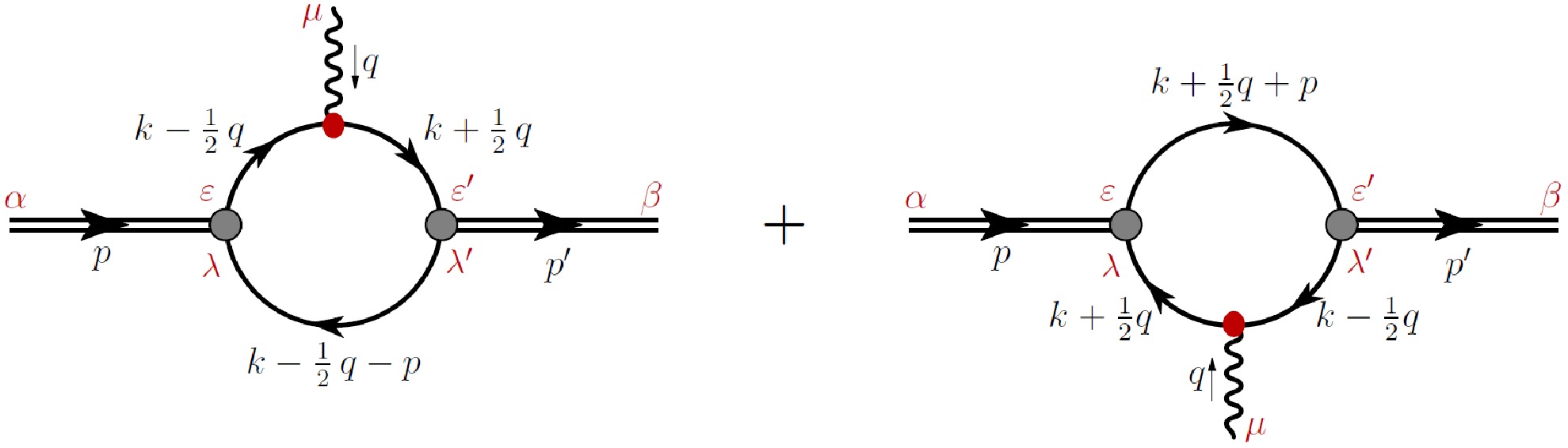
The off-shell GPDs of the pion in the NJL model are illustrated in Fig. 1. In this context, p represents the incoming pion momentum, while
$ p^{\prime} $ denotes the outgoing pion momentum. Unlike the on-shell case, we have$ p^2 \neq p^{\prime2} \neq m_{\pi}^2 $ . In this paper, we adopt the symmetry notation used in Refs. [7, 8]. The kinematics of this process and related quantities are defined as
Figure 1. (color online) Pion off-shell GPDs diagrams different from the pion on-shell GPDs in Ref. [10], here
$ p^2\neq p^{\prime2}\neq m_{\pi}^2 $ .$ t= q^2=(p'-p)^2=-Q^2, $
(10) $ \xi=\frac{p^+-p^{\prime+}}{p^++p^{\prime+}}, \quad P=\frac{p+p^{\prime}}{2}, $
(11) where ξ represents the skewness parameter, expressed in light-cone coordinates
$ v^{\pm}=(v^0\pm v^3), \quad {\boldsymbol{v}}=(v^1,v^2). $
(12) For any four-vector,
$ n=(1,0,0,-1) $ represents the light-cone four-vector, and$ v^+ $ in the light-cone coordinate can be expressed as$ v^+=v\cdot n. $
(13) These coordinates provide a natural framework for describing the infinite momentum frame, within which parton distributions can be elucidated through the physical perspective of the parton model.
The two leading-twist quark off-shell GPDs of the pion are defined as
$ \begin{aligned}[b] H(x,\xi,t,p^2,p^{\prime2}) =\;&\frac{1}{2}\int \frac{{\rm d}z^-}{2\pi}{\rm e}^{\tfrac{\rm i}{2}x(p^++p^{\prime+})z^-}\\ &\times \langle p^{\prime}|\bar{q}\left(-\frac{1}{2}z \right)\gamma^+q\left(\frac{1}{2}z\right)\big|p\rangle \mid_{z^+=0,{\boldsymbol{z}}={\boldsymbol{0}}}, \end{aligned} $
(14) $ \begin{aligned}[b] &\frac{P^+q^j-P^jq^+}{P^+m_{\pi}}E(x,\xi,t,p^2,p^{\prime2})\\ =\;&\frac{1}{2}\int \frac{{\rm d}z^-}{2\pi}{\rm e}^{\frac{\rm i}{2}x(p^++p^{\prime+})z^-}\\ &\times \langle p^{\prime}|\bar{q}\left(-\frac{1}{2}z\right){\rm i}\sigma^{+j}q\left(\frac{1}{2}z\right)|p\rangle \mid_{z^+=0,{\boldsymbol{z}}={\boldsymbol{0}}}, \end{aligned} $
(15) where x represents the longitudinal momentum fraction. The first is the vector (no spin flip) off-shell GPD, and the second is the tensor (spin flip) off-shell GPD. The operators for the two off-shell GPDs in Fig. 1 read
$ {\tag {16{\text{a}}}} \bullet_1 =\gamma^+\delta \left(x-\frac{k^++k^{\prime+}}{p^++p^{\prime+}}\right), $
$ {\tag {16{\text{b}}}} \bullet_2 ={\rm i}\sigma^{+j} \delta \left(x-\frac{k^++k^{\prime+}}{p^++p^{\prime+}}\right), $
$ \bullet_1 $ for vector off-shell GPD and$ \bullet_2 $ for tensor off-shell GPD.In the NJL model, the off-shell GPDs can be written as
$ \begin{aligned}[b] &H\left(x,\xi,t,p^2,p^{\prime 2}\right)\\[-2pt] =\;&2{\rm i} N_c Z_{\pi} \int \frac{{\rm d}^4k}{(2 \pi )^4}\delta_n^x (k)\\[-2pt] &\times {\rm{tr}}_{{\rm{D}}}\left[\gamma _5 S \left(k_{+q}\right)\gamma ^+ S\left(k_{-q}\right)\gamma _5 S\left(k-P\right)\right], \end{aligned} $
(17) $ \begin{aligned}[b] & \frac{P^+q^j-P^jq^+}{P^+m_{\pi}} E\left(x,\xi,t,p^2,p^{\prime 2}\right)\\[-2pt] =\;&2 {\rm i} N_c Z_{\pi}\int \frac{{\rm d}^4k}{(2 \pi )^4}\delta_n^x (k)\\[-2pt] &\times {\rm{tr}}_{{\rm{D}}}\left[\gamma _5 S \left(k_{+q}\right){\rm i}\sigma^{+j}S\left(k_{-q}\right)\gamma _5 S\left(k-P\right)\right], \end{aligned} $
(18) where
$ {\rm{tr}}_{{\rm{D}}} $ indicates a trace over spinor indices,$ \delta_n^x (k)= \delta (xP^+-k^+) $ ,$k_{+q}=k+ {q}/{2}$ , and$k_{-q}=k- {q}/{2}$ . Here, we use the reduce formulae ($ D(k^2)=k^2-M^2 $ )$ {\tag {19{\text{a}}}} p\cdot q=\frac{p^{\prime2}-p^2-q^2}{2}\,, $
$ {\tag {19{\text{b}}}} k\cdot q=\frac{1}{2} \left(D(k_{+q}^2)-D(k_{-q}^2)\right)\,, $
${\tag {19{\text{c}}}} k\cdot p=-\frac{1}{2} \left(D((k - P)^2)-D(k_{-q}^2) - \frac{p^{\prime2}+p^2- q^2}{2}\right)\,, $
${\tag {19{\text{d}}}} k^2=\frac{1}{2} \left(D(k_{+q}^2)+D(k_{-q}^2)\right)+M^2-\frac{q^2}{4}. $
To incorporate these relationships into Eqs. (17) and (18), we first cancel each identical factor in the numerators and denominators. Subsequently, by applying Feynman parametrizations to simplify all remaining denominators, we arrive at the following result
$ \begin{aligned}[b] & H(x,\xi,t,p^2,p^{\prime 2})\\[-2pt] =\;&\frac{N_cZ_{\pi }}{8\pi ^2} \left[\theta_{\bar{\xi} 1}\bar{{\cal{C}}}_1(\sigma_4)+ \theta_{\xi 1} \bar{{\cal{C}}}_1(\sigma_5)+\theta_{\bar{\xi} \xi}\frac{x}{\xi }\bar{{\cal{C}}}_1(\sigma_6)\right]\\[-2pt] &+\frac{N_c Z_{\pi } }{8\pi ^2}\int_0^1 {\rm d}\alpha \frac{\bar{{\cal{C}}}_2(\sigma_7)}{\sigma_7}\\[-2pt] &\times \frac{\theta_{\alpha \xi}\left((p^{\prime 2}-p^2)\xi+x(p^2+p^{\prime 2})+(1- x)t\right)}{\xi} , \end{aligned} $
(20) $ E(x,\xi,t,p^2,p^{\prime 2})=\frac{N_c Z_{\pi } }{4\pi ^2}\int_0^1 {\rm d}\alpha \frac{\theta_{\alpha \xi}}{\xi}m_{\pi}M\frac{\bar{{\cal{C}}}_2(\sigma_7)}{\sigma_7}, $
(21) and
${\tag {22{\text{a}}}} \theta_{\bar{\xi} 1}=x\in[-\xi, 1]\,, $
$ {\tag {22{\text{b}}}} \theta_{\xi 1}=x\in[\xi, 1]\,, $
$ {\tag {22{\text{c}}}} \theta_{\bar{\xi} \xi}=x\in[-\xi, \xi]\,, $
${\tag {22{\text{d}}}} \theta_{\alpha \xi}=x\in[\alpha (\xi +1)-\xi , \alpha (1-\xi)+\xi ]\cap x\in[-1,1], $
the step function θ indicates that x exists solely within the corresponding region. One can express
$ \theta_{\bar{\xi} \xi}/\xi = \Theta(1 - x^2/\xi^2) $ , where$ \Theta(x) $ represents the Heaviside function. In addition, we have$ \theta_{\alpha \xi}/\xi = \Theta((1 - \alpha^2) - (x - \alpha)^2/\xi^2)\Theta(1 - x^2) $ . These results are valid in the region where$ \xi > 0 $ . Under the transformation$ \xi \rightarrow -\xi $ , it follows that$ \theta_{\bar{\xi} 1} \leftrightarrow \theta_{\xi 1} $ , and both$ \theta_{\bar{\xi} \xi}/\xi $ and$ \theta_{\alpha \xi}/\xi $ remain invariant.Here, we present the diagrams of
$ H(x,\xi,t,p^2,m_{\pi}^2) $ and$ E(x,\xi,t,p^2,m_{\pi}^2) $ in Figs. 2 and 3. The functions$ H(x,0.5,0, m_{\pi}^2,m_{\pi}^2) $ and$ E(x,0.5,0,m_{\pi}^2,m_{\pi}^2) $ , which correspond to the on-shell GPDs, are discussed in Ref. [10]. In this study, we plot the on-shell vector and tensor GPDs for a comparative analysis.
Figure 2. (color online) Pion off-shell vector GPD
$ H(x, \xi, t, p^2, $ $ p^{\prime 2}) $ in Eq. (24), we only plot$ \xi>0 $ . Upper panel –$ H(x, 0.5, 0, p^2, $ $ m_\pi^2) $ . Lower-panel –$ H(x,0.5,-1,p^2,m_\pi^2) $ . In both cases,$ p^2 = m_\pi^2 $ $ {\rm GeV}^2 $ – black dotted;$ p^2=0\; {\rm GeV}^2 $ – red solid line;$ p^2=0.2 $ $ {\rm GeV}^2 $ – blue dashed line; and$ p^2=0.4 \;{\rm GeV}^2 $ – purple dot-dashed line.
Figure 3. (color online) Pion off-shell tensor GPD
$ E(x,\xi,t,p^2, $ $ p^{\prime 2}) $ in Eq. (25), we only plot$ \xi>0 $ . Upper panel –$ E(x,0.5,0,p^2, $ $ m_\pi^2) $ . Lower-panel –$ E(x,0.5,-1,p^2, m_\pi^2) $ . In both cases,$ p^2 = m_\pi^2 $ $ {\rm GeV}^2$ – black dotted;$ p^2=0 \;{\rm GeV}^2 $ – red solid line;$ p^2=0.2 $ $ {\rm GeV}^2$ – blue dashed line; and$ p^2=0.4 \;{\rm GeV}^2 $ – purple dot-dashed line.The diagrams indicate that, when
$ p^{\prime 2}=m_{\pi}^{2} $ , the off-shellness depends on$ p^{2} $ . As$ p^{2} $ increases, the off-shell effects of half-off-shell pion GPDs become more pronounced. Specifically, at$ p^{2}=0.2 $ GeV2, the relative effect is approximately 15% for the maximum value, while at a higher value of$ p^{2}=0.4 $ GeV2, this relative effect rises to about 25%. -
The off-shell GPDs of the pion in the NJL model are illustrated in Fig. 1. In this context, p represents the incoming pion momentum, while
$ p^{\prime} $ denotes the outgoing pion momentum. Unlike the on-shell case, we have$ p^2 \neq p^{\prime2} \neq m_{\pi}^2 $ . In this paper, we adopt the symmetry notation used in Refs. [7, 8]. The kinematics of this process and related quantities are defined as
Figure 1. (color online) Pion off-shell GPDs diagrams different from the pion on-shell GPDs in Ref. [10], here
$ p^2\neq p^{\prime2}\neq m_{\pi}^2 $ .$ t= q^2=(p'-p)^2=-Q^2, $
(10) $ \xi=\frac{p^+-p^{\prime+}}{p^++p^{\prime+}}, \quad P=\frac{p+p^{\prime}}{2}, $
(11) where ξ represents the skewness parameter, expressed in light-cone coordinates
$ v^{\pm}=(v^0\pm v^3), \quad {\boldsymbol{v}}=(v^1,v^2). $
(12) For any four-vector,
$ n=(1,0,0,-1) $ represents the light-cone four-vector, and$ v^+ $ in the light-cone coordinate can be expressed as$ v^+=v\cdot n. $
(13) These coordinates provide a natural framework for describing the infinite momentum frame, within which parton distributions can be elucidated through the physical perspective of the parton model.
The two leading-twist quark off-shell GPDs of the pion are defined as
$ \begin{aligned}[b] H(x,\xi,t,p^2,p^{\prime2}) =\;&\frac{1}{2}\int \frac{{\rm d}z^-}{2\pi}{\rm e}^{\tfrac{\rm i}{2}x(p^++p^{\prime+})z^-}\\ &\times \langle p^{\prime}|\bar{q}\left(-\frac{1}{2}z \right)\gamma^+q\left(\frac{1}{2}z\right)\big|p\rangle \mid_{z^+=0,{\boldsymbol{z}}={\boldsymbol{0}}}, \end{aligned} $
(14) $ \begin{aligned}[b] &\frac{P^+q^j-P^jq^+}{P^+m_{\pi}}E(x,\xi,t,p^2,p^{\prime2})\\ =\;&\frac{1}{2}\int \frac{{\rm d}z^-}{2\pi}{\rm e}^{\frac{\rm i}{2}x(p^++p^{\prime+})z^-}\\ &\times \langle p^{\prime}|\bar{q}\left(-\frac{1}{2}z\right){\rm i}\sigma^{+j}q\left(\frac{1}{2}z\right)|p\rangle \mid_{z^+=0,{\boldsymbol{z}}={\boldsymbol{0}}}, \end{aligned} $
(15) where x represents the longitudinal momentum fraction. The first is the vector (no spin flip) off-shell GPD, and the second is the tensor (spin flip) off-shell GPD. The operators for the two off-shell GPDs in Fig. 1 read
$ \bullet_1 =\gamma^+\delta \left(x-\frac{k^++k^{\prime+}}{p^++p^{\prime+}}\right), $
(16a) $ \bullet_2 ={\rm i}\sigma^{+j} \delta \left(x-\frac{k^++k^{\prime+}}{p^++p^{\prime+}}\right), $
(16b) $ \bullet_1 $ for vector off-shell GPD and$ \bullet_2 $ for tensor off-shell GPD.In the NJL model, the off-shell GPDs can be written as
$ \begin{aligned}[b] &H\left(x,\xi,t,p^2,p^{\prime 2}\right)\\[-2pt] =\;&2{\rm i} N_c Z_{\pi} \int \frac{{\rm d}^4k}{(2 \pi )^4}\delta_n^x (k)\\[-2pt] &\times {\rm{tr}}_{{\rm{D}}}\left[\gamma _5 S \left(k_{+q}\right)\gamma ^+ S\left(k_{-q}\right)\gamma _5 S\left(k-P\right)\right], \end{aligned} $
(17) $ \begin{aligned}[b] & \frac{P^+q^j-P^jq^+}{P^+m_{\pi}} E\left(x,\xi,t,p^2,p^{\prime 2}\right)\\[-2pt] =\;&2 {\rm i} N_c Z_{\pi}\int \frac{{\rm d}^4k}{(2 \pi )^4}\delta_n^x (k)\\[-2pt] &\times {\rm{tr}}_{{\rm{D}}}\left[\gamma _5 S \left(k_{+q}\right){\rm i}\sigma^{+j}S\left(k_{-q}\right)\gamma _5 S\left(k-P\right)\right], \end{aligned} $
(18) where
$ {\rm{tr}}_{{\rm{D}}} $ indicates a trace over spinor indices,$ \delta_n^x (k)= \delta (xP^+-k^+) $ ,$k_{+q}=k+ {q}/{2}$ , and$k_{-q}=k- {q}/{2}$ . Here, we use the reduce formulae ($ D(k^2)=k^2-M^2 $ )$p\cdot q=\frac{p^{\prime2}-p^2-q^2}{2}\,, $
(19a) $ k\cdot q=\frac{1}{2} \left(D(k_{+q}^2)-D(k_{-q}^2)\right)\,, $
(19b) $ k\cdot p=-\frac{1}{2} \left(D((k - P)^2)-D(k_{-q}^2) - \frac{p^{\prime2}+p^2- q^2}{2}\right)\,, $
(19c) $ k^2=\frac{1}{2} \left(D(k_{+q}^2)+D(k_{-q}^2)\right)+M^2-\frac{q^2}{4}. $
(19d) To incorporate these relationships into Eqs. (17) and (18), we first cancel each identical factor in the numerators and denominators. Subsequently, by applying Feynman parametrizations to simplify all remaining denominators, we arrive at the following result
$ \begin{aligned}[b] & H(x,\xi,t,p^2,p^{\prime 2})\\[-2pt] =\;&\frac{N_cZ_{\pi }}{8\pi ^2} \left[\theta_{\bar{\xi} 1}\bar{{\cal{C}}}_1(\sigma_4)+ \theta_{\xi 1} \bar{{\cal{C}}}_1(\sigma_5)+\theta_{\bar{\xi} \xi}\frac{x}{\xi }\bar{{\cal{C}}}_1(\sigma_6)\right]\\[-2pt] &+\frac{N_c Z_{\pi } }{8\pi ^2}\int_0^1 {\rm d}\alpha \frac{\bar{{\cal{C}}}_2(\sigma_7)}{\sigma_7}\\[-2pt] &\times \frac{\theta_{\alpha \xi}\left((p^{\prime 2}-p^2)\xi+x(p^2+p^{\prime 2})+(1- x)t\right)}{\xi} , \end{aligned} $
(20) $ E(x,\xi,t,p^2,p^{\prime 2})=\frac{N_c Z_{\pi } }{4\pi ^2}\int_0^1 {\rm d}\alpha \frac{\theta_{\alpha \xi}}{\xi}m_{\pi}M\frac{\bar{{\cal{C}}}_2(\sigma_7)}{\sigma_7}, $
(21) and
$ \theta_{\bar{\xi} 1}=x\in[-\xi, 1]\,, $
(22a) $ \theta_{\xi 1}=x\in[\xi, 1]\,, $
(22b) $ \theta_{\bar{\xi} \xi}=x\in[-\xi, \xi]\,, $
(22c) $ \theta_{\alpha \xi}=x\in[\alpha (\xi +1)-\xi , \alpha (1-\xi)+\xi ]\cap x\in[-1,1], $
(22d) the step function θ indicates that x exists solely within the corresponding region. One can express
$ \theta_{\bar{\xi} \xi}/\xi = \Theta(1 - x^2/\xi^2) $ , where$ \Theta(x) $ represents the Heaviside function. In addition, we have$ \theta_{\alpha \xi}/\xi = \Theta((1 - \alpha^2) - (x - \alpha)^2/\xi^2)\Theta(1 - x^2) $ . These results are valid in the region where$ \xi \gt 0 $ . Under the transformation$ \xi \rightarrow -\xi $ , it follows that$ \theta_{\bar{\xi} 1} \leftrightarrow \theta_{\xi 1} $ , and both$ \theta_{\bar{\xi} \xi}/\xi $ and$ \theta_{\alpha \xi}/\xi $ remain invariant.Here, we present the diagrams of
$ H(x,\xi,t,p^2,m_{\pi}^2) $ and$ E(x,\xi,t,p^2,m_{\pi}^2) $ in Figs. 2 and 3. The functions$ H(x,0.5,0, m_{\pi}^2,m_{\pi}^2) $ and$ E(x,0.5,0,m_{\pi}^2,m_{\pi}^2) $ , which correspond to the on-shell GPDs, are discussed in Ref. [10]. In this study, we plot the on-shell vector and tensor GPDs for a comparative analysis.
Figure 2. (color online) Pion off-shell vector GPD
$ H(x, \xi, t, p^2, $ $ p^{\prime 2}) $ in Eq. (24), we only plot$ \xi>0 $ . Upper panel –$ H(x, 0.5, 0, p^2, $ $ m_\pi^2) $ . Lower-panel –$ H(x,0.5,-1,p^2,m_\pi^2) $ . In both cases,$ p^2 = m_\pi^2 $ $ {\rm GeV}^2 $ – black dotted;$ p^2=0\; {\rm GeV}^2 $ – red solid line;$ p^2=0.2 $ $ {\rm GeV}^2 $ – blue dashed line; and$ p^2=0.4 \;{\rm GeV}^2 $ – purple dot-dashed line.
Figure 3. (color online) Pion off-shell tensor GPD
$ E(x,\xi,t,p^2, $ $ p^{\prime 2}) $ in Eq. (25), we only plot$ \xi>0 $ . Upper panel –$ E(x,0.5,0,p^2, $ $ m_\pi^2) $ . Lower-panel –$ E(x,0.5,-1,p^2, m_\pi^2) $ . In both cases,$ p^2 = m_\pi^2 $ $ {\rm GeV}^2$ – black dotted;$ p^2=0 \;{\rm GeV}^2 $ – red solid line;$ p^2=0.2 $ $ {\rm GeV}^2$ – blue dashed line; and$ p^2=0.4 \;{\rm GeV}^2 $ – purple dot-dashed line.The diagrams indicate that, when
$ p^{\prime 2}=m_{\pi}^{2} $ , the off-shellness depends on$ p^{2} $ . As$ p^{2} $ increases, the off-shell effects of half-off-shell pion GPDs become more pronounced. Specifically, at$ p^{2}=0.2 $ GeV2, the relative effect is approximately 15% for the maximum value, while at a higher value of$ p^{2}=0.4 $ GeV2, this relative effect rises to about 25%. -
The off-shell GPDs of the pion in the NJL model are illustrated in Fig. 1. In this context, p represents the incoming pion momentum, while
$ p^{\prime} $ denotes the outgoing pion momentum. Unlike the on-shell case, we have$ p^2 \neq p^{\prime2} \neq m_{\pi}^2 $ . In this paper, we adopt the symmetry notation used in Refs. [7, 8]. The kinematics of this process and related quantities are defined as
Figure 1. (color online) Pion off-shell GPDs diagrams different from the pion on-shell GPDs in Ref. [10], here
$ p^2\neq p^{\prime2}\neq m_{\pi}^2 $ .$ t= q^2=(p'-p)^2=-Q^2, $
(10) $ \xi=\frac{p^+-p^{\prime+}}{p^++p^{\prime+}}, \quad P=\frac{p+p^{\prime}}{2}, $
(11) where ξ represents the skewness parameter, expressed in light-cone coordinates
$ v^{\pm}=(v^0\pm v^3), \quad {\boldsymbol{v}}=(v^1,v^2). $
(12) For any four-vector,
$ n=(1,0,0,-1) $ represents the light-cone four-vector, and$ v^+ $ in the light-cone coordinate can be expressed as$ v^+=v\cdot n. $
(13) These coordinates provide a natural framework for describing the infinite momentum frame, within which parton distributions can be elucidated through the physical perspective of the parton model.
The two leading-twist quark off-shell GPDs of the pion are defined as
$ \begin{aligned}[b] H(x,\xi,t,p^2,p^{\prime2}) =\;&\frac{1}{2}\int \frac{{\rm d}z^-}{2\pi}{\rm e}^{\tfrac{\rm i}{2}x(p^++p^{\prime+})z^-}\\ &\times \langle p^{\prime}|\bar{q}\left(-\frac{1}{2}z \right)\gamma^+q\left(\frac{1}{2}z\right)\big|p\rangle \mid_{z^+=0,{\boldsymbol{z}}={\boldsymbol{0}}}, \end{aligned} $
(14) $ \begin{aligned}[b] &\frac{P^+q^j-P^jq^+}{P^+m_{\pi}}E(x,\xi,t,p^2,p^{\prime2})\\ =\;&\frac{1}{2}\int \frac{{\rm d}z^-}{2\pi}{\rm e}^{\frac{\rm i}{2}x(p^++p^{\prime+})z^-}\\ &\times \langle p^{\prime}|\bar{q}\left(-\frac{1}{2}z\right){\rm i}\sigma^{+j}q\left(\frac{1}{2}z\right)|p\rangle \mid_{z^+=0,{\boldsymbol{z}}={\boldsymbol{0}}}, \end{aligned} $
(15) where x represents the longitudinal momentum fraction. The first is the vector (no spin flip) off-shell GPD, and the second is the tensor (spin flip) off-shell GPD. The operators for the two off-shell GPDs in Fig. 1 read
$ {\tag {16{\text{a}}}} \bullet_1 =\gamma^+\delta \left(x-\frac{k^++k^{\prime+}}{p^++p^{\prime+}}\right), $
$ {\tag {16{\text{b}}}} \bullet_2 ={\rm i}\sigma^{+j} \delta \left(x-\frac{k^++k^{\prime+}}{p^++p^{\prime+}}\right), $
$ \bullet_1 $ for vector off-shell GPD and$ \bullet_2 $ for tensor off-shell GPD.In the NJL model, the off-shell GPDs can be written as
$ \begin{aligned}[b] &H\left(x,\xi,t,p^2,p^{\prime 2}\right)\\[-2pt] =\;&2{\rm i} N_c Z_{\pi} \int \frac{{\rm d}^4k}{(2 \pi )^4}\delta_n^x (k)\\[-2pt] &\times {\rm{tr}}_{{\rm{D}}}\left[\gamma _5 S \left(k_{+q}\right)\gamma ^+ S\left(k_{-q}\right)\gamma _5 S\left(k-P\right)\right], \end{aligned} $
(17) $ \begin{aligned}[b] & \frac{P^+q^j-P^jq^+}{P^+m_{\pi}} E\left(x,\xi,t,p^2,p^{\prime 2}\right)\\[-2pt] =\;&2 {\rm i} N_c Z_{\pi}\int \frac{{\rm d}^4k}{(2 \pi )^4}\delta_n^x (k)\\[-2pt] &\times {\rm{tr}}_{{\rm{D}}}\left[\gamma _5 S \left(k_{+q}\right){\rm i}\sigma^{+j}S\left(k_{-q}\right)\gamma _5 S\left(k-P\right)\right], \end{aligned} $
(18) where
$ {\rm{tr}}_{{\rm{D}}} $ indicates a trace over spinor indices,$ \delta_n^x (k)= \delta (xP^+-k^+) $ ,$k_{+q}=k+ {q}/{2}$ , and$k_{-q}=k- {q}/{2}$ . Here, we use the reduce formulae ($ D(k^2)=k^2-M^2 $ )$ {\tag {19{\text{a}}}} p\cdot q=\frac{p^{\prime2}-p^2-q^2}{2}\,, $
$ {\tag {19{\text{b}}}} k\cdot q=\frac{1}{2} \left(D(k_{+q}^2)-D(k_{-q}^2)\right)\,, $
${\tag {19{\text{c}}}} k\cdot p=-\frac{1}{2} \left(D((k - P)^2)-D(k_{-q}^2) - \frac{p^{\prime2}+p^2- q^2}{2}\right)\,, $
${\tag {19{\text{d}}}} k^2=\frac{1}{2} \left(D(k_{+q}^2)+D(k_{-q}^2)\right)+M^2-\frac{q^2}{4}. $
To incorporate these relationships into Eqs. (17) and (18), we first cancel each identical factor in the numerators and denominators. Subsequently, by applying Feynman parametrizations to simplify all remaining denominators, we arrive at the following result
$ \begin{aligned}[b] & H(x,\xi,t,p^2,p^{\prime 2})\\[-2pt] =\;&\frac{N_cZ_{\pi }}{8\pi ^2} \left[\theta_{\bar{\xi} 1}\bar{{\cal{C}}}_1(\sigma_4)+ \theta_{\xi 1} \bar{{\cal{C}}}_1(\sigma_5)+\theta_{\bar{\xi} \xi}\frac{x}{\xi }\bar{{\cal{C}}}_1(\sigma_6)\right]\\[-2pt] &+\frac{N_c Z_{\pi } }{8\pi ^2}\int_0^1 {\rm d}\alpha \frac{\bar{{\cal{C}}}_2(\sigma_7)}{\sigma_7}\\[-2pt] &\times \frac{\theta_{\alpha \xi}\left((p^{\prime 2}-p^2)\xi+x(p^2+p^{\prime 2})+(1- x)t\right)}{\xi} , \end{aligned} $
(20) $ E(x,\xi,t,p^2,p^{\prime 2})=\frac{N_c Z_{\pi } }{4\pi ^2}\int_0^1 {\rm d}\alpha \frac{\theta_{\alpha \xi}}{\xi}m_{\pi}M\frac{\bar{{\cal{C}}}_2(\sigma_7)}{\sigma_7}, $
(21) and
${\tag {22{\text{a}}}} \theta_{\bar{\xi} 1}=x\in[-\xi, 1]\,, $
$ {\tag {22{\text{b}}}} \theta_{\xi 1}=x\in[\xi, 1]\,, $
$ {\tag {22{\text{c}}}} \theta_{\bar{\xi} \xi}=x\in[-\xi, \xi]\,, $
${\tag {22{\text{d}}}} \theta_{\alpha \xi}=x\in[\alpha (\xi +1)-\xi , \alpha (1-\xi)+\xi ]\cap x\in[-1,1], $
the step function θ indicates that x exists solely within the corresponding region. One can express
$ \theta_{\bar{\xi} \xi}/\xi = \Theta(1 - x^2/\xi^2) $ , where$ \Theta(x) $ represents the Heaviside function. In addition, we have$ \theta_{\alpha \xi}/\xi = \Theta((1 - \alpha^2) - (x - \alpha)^2/\xi^2)\Theta(1 - x^2) $ . These results are valid in the region where$ \xi > 0 $ . Under the transformation$ \xi \rightarrow -\xi $ , it follows that$ \theta_{\bar{\xi} 1} \leftrightarrow \theta_{\xi 1} $ , and both$ \theta_{\bar{\xi} \xi}/\xi $ and$ \theta_{\alpha \xi}/\xi $ remain invariant.Here, we present the diagrams of
$ H(x,\xi,t,p^2,m_{\pi}^2) $ and$ E(x,\xi,t,p^2,m_{\pi}^2) $ in Figs. 2 and 3. The functions$ H(x,0.5,0, m_{\pi}^2,m_{\pi}^2) $ and$ E(x,0.5,0,m_{\pi}^2,m_{\pi}^2) $ , which correspond to the on-shell GPDs, are discussed in Ref. [10]. In this study, we plot the on-shell vector and tensor GPDs for a comparative analysis.
Figure 2. (color online) Pion off-shell vector GPD
$ H(x, \xi, t, p^2, $ $ p^{\prime 2}) $ in Eq. (24), we only plot$ \xi>0 $ . Upper panel –$ H(x, 0.5, 0, p^2, $ $ m_\pi^2) $ . Lower-panel –$ H(x,0.5,-1,p^2,m_\pi^2) $ . In both cases,$ p^2 = m_\pi^2 $ $ {\rm GeV}^2 $ – black dotted;$ p^2=0\; {\rm GeV}^2 $ – red solid line;$ p^2=0.2 $ $ {\rm GeV}^2 $ – blue dashed line; and$ p^2=0.4 \;{\rm GeV}^2 $ – purple dot-dashed line.
Figure 3. (color online) Pion off-shell tensor GPD
$ E(x,\xi,t,p^2, $ $ p^{\prime 2}) $ in Eq. (25), we only plot$ \xi>0 $ . Upper panel –$ E(x,0.5,0,p^2, $ $ m_\pi^2) $ . Lower-panel –$ E(x,0.5,-1,p^2, m_\pi^2) $ . In both cases,$ p^2 = m_\pi^2 $ $ {\rm GeV}^2$ – black dotted;$ p^2=0 \;{\rm GeV}^2 $ – red solid line;$ p^2=0.2 $ $ {\rm GeV}^2$ – blue dashed line; and$ p^2=0.4 \;{\rm GeV}^2 $ – purple dot-dashed line.The diagrams indicate that, when
$ p^{\prime 2}=m_{\pi}^{2} $ , the off-shellness depends on$ p^{2} $ . As$ p^{2} $ increases, the off-shell effects of half-off-shell pion GPDs become more pronounced. Specifically, at$ p^{2}=0.2 $ GeV2, the relative effect is approximately 15% for the maximum value, while at a higher value of$ p^{2}=0.4 $ GeV2, this relative effect rises to about 25%. -
The off-shell GPDs of the pion in the NJL model are illustrated in Fig. 1. In this context, p represents the incoming pion momentum, while
$ p^{\prime} $ denotes the outgoing pion momentum. Unlike the on-shell case, we have$ p^2 \neq p^{\prime2} \neq m_{\pi}^2 $ . In this paper, we will adopt the symmetry notation as used in Refs. [7, 8]. The kinematics of this process and related quantities are defined as follows:
Figure 1. (color online) Pion off-shell GPDs diagrams, different from the pion on-shell GPDs in Ref. [10], here
$ p^2\neq p^{\prime2}\neq m_{\pi}^2 $ .$ t= q^2=(p'-p)^2=-Q^2, $
(10) $ \xi=\frac{p^+-p^{\prime+}}{p^++p^{\prime+}}, \quad P=\frac{p+p^{\prime}}{2}, $
(11) where ξ represents the skewness parameter, expressed in light-cone coordinates
$ v^{\pm}=(v^0\pm v^3), \quad {\bf{v}}=(v^1,v^2), $
(12) for any four-vector,
$ n=(1,0,0,-1) $ is the light-cone four-vector, then$ v^+ $ in the light-cone coordinate can be expressed as follows:$ v^+=v\cdot n. $
(13) These coordinates provide a natural framework for describing the infinite momentum frame, within which parton distributions can be elucidated through the physical perspective of the parton model.
The two leading-twist quark off-shell GPDs of the pion are defined as follows:
$ \begin{aligned}[b] H(x,\xi,t,p^2,p^{\prime2}) =\;&\frac{1}{2}\int \frac{dz^-}{2\pi}e^{\tfrac{i}{2}x(p^++p^{\prime+})z^-}\\ &\times \langle p^{\prime}|\bar{q}\left(-\frac{1}{2}z \right)\gamma^+q\left(\frac{1}{2}z\right)|p\rangle \mid_{z^+=0,{\boldsymbol{z}}={\boldsymbol{0}}}, \end{aligned} $
(14) $ \begin{aligned}[b] &\frac{P^+q^j-P^jq^+}{P^+m_{\pi}}E(x,\xi,t,p^2,p^{\prime2})\\ =\;&\frac{1}{2}\int \frac{dz^-}{2\pi}e^{\frac{i}{2}x(p^++p^{\prime+})z^-}\\ &\times \langle p^{\prime}|\bar{q}\left(-\frac{1}{2}z\right)i\sigma^{+j}q\left(\frac{1}{2}z\right)|p\rangle \mid_{z^+=0,{\boldsymbol{z}}={\boldsymbol{0}}}, \end{aligned} $
(15) where x is the longitudinal momentum fraction. The first is the vector (no spin flip) off-shell GPD, the second is tensor (spin flip) off-shell GPD. The operators for the two off-shell GPDs in Fig. 1 read
$ {\tag {16{\text{a}}}} \bullet_1 =\gamma^+\delta(x-\frac{k^++k^{\prime+}}{p^++p^{\prime+}})\,, $
$ {\tag {16{\text{b}}}} \bullet_2 =i\sigma^{+j} \delta(x-\frac{k^++k^{\prime+}}{p^++p^{\prime+}}), $
$ \bullet_1 $ for vector off-shell GPD and$ \bullet_2 $ for tensor off-shell GPD.In the NJL model the off-shell GPDs can be written as
$ \begin{aligned}[b] &H\left(x,\xi,t,p^2,p^{\prime 2}\right)\\[-2pt] =\;&2i N_c Z_{\pi} \int \frac{d^4k}{(2 \pi )^4}\delta_n^x (k)\\[-2pt] &\times {\rm{tr}}_{{\rm{D}}}\left[\gamma _5 S \left(k_{+q}\right)\gamma ^+ S\left(k_{-q}\right)\gamma _5 S\left(k-P\right)\right], \end{aligned} $
(17) $ \begin{aligned}[b] & \frac{P^+q^j-P^jq^+}{P^+m_{\pi}} E\left(x,\xi,t,p^2,p^{\prime 2}\right)\\[-2pt] =\;&2i N_c Z_{\pi}\int \frac{d^4k}{(2 \pi )^4}\delta_n^x (k)\\[-2pt] &\times {\rm{tr}}_{{\rm{D}}}\left[\gamma _5 S \left(k_{+q}\right)i\sigma^{+j}S\left(k_{-q}\right)\gamma _5 S\left(k-P\right)\right], \end{aligned} $
(18) where
$ {\rm{tr}}_{{\rm{D}}} $ indicates a trace over spinor indices,$ \delta_n^x (k)=\delta (xP^+-k^+) $ ,$ k_{+q}=k+\frac{q}{2} $ ,$ k_{-q}=k-\frac{q}{2} $ . Here we use the following reduce formulae ($ D(k^2)=k^2-M^2 $ )$ {\tag {19{\text{a}}}} p\cdot q=\frac{p^{\prime2}-p^2-q^2}{2}\,, $
$ {\tag {19{\text{b}}}} k\cdot q=\frac{1}{2} \left(D(k_{+q}^2)-D(k_{-q}^2)\right)\,, $
${\tag {19{\text{c}}}} k\cdot p=-\frac{1}{2} \left(D((k - P)^2)-D(k_{-q}^2) - \frac{p^{\prime2}+p^2- q^2}{2}\right)\,, $
${\tag {19{\text{d}}}} k^2=\frac{1}{2} \left(D(k_{+q}^2)+D(k_{-q}^2)\right)+M^2-\frac{q^2}{4}, $
to incorporate these relationships into Eqs. (18) and (19), we first cancel each identical factor in the numerators and denominators. Subsequently, by applying Feynman parametrizations to simplify all remaining denominators, we arrive at the following result:
$ \begin{aligned}[b] & H(x,\xi,t,p^2,p^{\prime 2})\\[-2pt] =\;&\frac{N_cZ_{\pi }}{8\pi ^2} \left[\theta_{\bar{\xi} 1}\bar{{\cal{C}}}_1(\sigma_4)+ \theta_{\xi 1} \bar{{\cal{C}}}_1(\sigma_5)+\theta_{\bar{\xi} \xi}\frac{x}{\xi }\bar{{\cal{C}}}_1(\sigma_6)\right]\\[-2pt] &+\frac{N_c Z_{\pi } }{8\pi ^2}\int_0^1 d\alpha \frac{\bar{{\cal{C}}}_2(\sigma_7)}{\sigma_7}\\[-2pt] &\times \frac{\theta_{\alpha \xi}\left((p^{\prime 2}-p^2)\xi+x(p^2+p^{\prime 2})+(1- x)t\right)}{\xi} , \end{aligned} $
(20) $ E(x,\xi,t,p^2,p^{\prime 2})=\frac{N_c Z_{\pi } }{4\pi ^2}\int_0^1 d\alpha \frac{\theta_{\alpha \xi}}{\xi}m_{\pi}M\frac{\bar{{\cal{C}}}_2(\sigma_7)}{\sigma_7}, $
(21) and
${\tag {22{\text{a}}}} \theta_{\bar{\xi} 1}=x\in[-\xi, 1]\,, $
$ {\tag {22{\text{b}}}} \theta_{\xi 1}=x\in[\xi, 1]\,, $
$ {\tag {22{\text{c}}}} \theta_{\bar{\xi} \xi}=x\in[-\xi, \xi]\,, $
${\tag {22{\text{d}}}} \theta_{\alpha \xi}=x\in[\alpha (\xi +1)-\xi , \alpha (1-\xi)+\xi ]\cap x\in[-1,1], $
the step function θ indicates that x exists solely within the corresponding region. One can express
$ \theta_{\bar{\xi} \xi}/\xi = \Theta(1 - x^2/\xi^2) $ , where$ \Theta(x) $ denotes the Heaviside function. Additionally, we have$ \theta_{\alpha \xi}/\xi = \Theta((1 - \alpha^2) - (x - \alpha)^2/\xi^2)\Theta(1 - x^2) $ . These results are valid in the region where$ \xi > 0 $ . Under the transformation$ \xi \rightarrow -\xi $ , it follows that:$ \theta_{\bar{\xi} 1} \leftrightarrow \theta_{\xi 1} $ ; and both$ \theta_{\bar{\xi} \xi}/\xi $ and$ \theta_{\alpha \xi}/\xi $ remain invariant.Here, we present the diagrams of
$ H(x,\xi,t,p^2,m_{\pi}^2) $ and$ E(x,\xi,t,p^2,m_{\pi}^2) $ in Figs. 2 and 3. The functions$ H(x,0.5,0, m_{\pi}^2,m_{\pi}^2) $ and$ E(x,0.5,0,m_{\pi}^2,m_{\pi}^2) $ , which correspond to the on-shell GPDs, are discussed in Ref. [10]. In this work, we also plot the on-shell vector and tensor GPDs for comparative analysis.
Figure 2. (color online) Pion off-shell vector GPD
$ H(x,\xi,t,p^2,p^{\prime 2}) $ in Eq. (24), we only plot$ \xi>0 $ . Upper panel –$ H(x,0.5,0,p^2,m_\pi^2) $ . Lower-panel -$ H(x,0.5,-1,p^2,m_\pi^2) $ . In both cases,$ p^2 = m_\pi^2 $ – black dotted;$ p^2=0 $ – red solid line;$ p^2=0.2 $ – blue dashed line;$ p^2=0.4 $ – purple dotdashed line.
Figure 3. (color online) Pion off-shell tensor GPD
$ E(x,\xi,t,p^2,p^{\prime 2}) $ in Eq. (25), we only plot$ \xi>0 $ . Upper panel –$ E(x,0.5,0,p^2,m_\pi^2) $ . Lower-panel -$ E(x,0.5,-1,p^2,m_\pi^2) $ . In both cases,$ p^2 = m_\pi^2 $ – black dotted;$ p^2=0 $ – red solid line;$ p^2=0.2 $ – blue dashed line;$ p^2=0.4 $ – purple dotdashed line.From the diagrams, it is evident that when
$ p^{\prime 2}=m_{\pi}^{2} $ , the off-shellness depends on$ p^{2} $ . As$ p^{2} $ increases, the off-shell effects of half-off-shell pion GPDs become more pronounced. Specifically, at$ p^{2}=0.2 $ GeV2, the relative effect is approximately 15% for the maximum value, while at a higher value of$ p^{2}=0.4 $ GeV2, this relative effect rises to about 25%. -
The off-shell GPDs of the pion in the NJL model are illustrated in Fig. 1. In this context, p represents the incoming pion momentum, while
$ p^{\prime} $ denotes the outgoing pion momentum. Unlike the on-shell case, we have$ p^2 \neq p^{\prime2} \neq m_{\pi}^2 $ . In this paper, we adopt the symmetry notation used in Refs. [7, 8]. The kinematics of this process and related quantities are defined as
Figure 1. (color online) Pion off-shell GPDs diagrams different from the pion on-shell GPDs in Ref. [10], here
$ p^2\neq p^{\prime2}\neq m_{\pi}^2 $ .$ t= q^2=(p'-p)^2=-Q^2, $
(10) $ \xi=\frac{p^+-p^{\prime+}}{p^++p^{\prime+}}, \quad P=\frac{p+p^{\prime}}{2}, $
(11) where ξ represents the skewness parameter, expressed in light-cone coordinates
$ v^{\pm}=(v^0\pm v^3), \quad {\boldsymbol{v}}=(v^1,v^2). $
(12) For any four-vector,
$ n=(1,0,0,-1) $ represents the light-cone four-vector, and$ v^+ $ in the light-cone coordinate can be expressed as$ v^+=v\cdot n. $
(13) These coordinates provide a natural framework for describing the infinite momentum frame, within which parton distributions can be elucidated through the physical perspective of the parton model.
The two leading-twist quark off-shell GPDs of the pion are defined as
$ \begin{aligned}[b] H(x,\xi,t,p^2,p^{\prime2}) =\;&\frac{1}{2}\int \frac{{\rm d}z^-}{2\pi}{\rm e}^{\tfrac{\rm i}{2}x(p^++p^{\prime+})z^-}\\ &\times \langle p^{\prime}|\bar{q}\left(-\frac{1}{2}z \right)\gamma^+q\left(\frac{1}{2}z\right)\big|p\rangle \mid_{z^+=0,{\boldsymbol{z}}={\boldsymbol{0}}}, \end{aligned} $
(14) $ \begin{aligned}[b] &\frac{P^+q^j-P^jq^+}{P^+m_{\pi}}E(x,\xi,t,p^2,p^{\prime2})\\ =\;&\frac{1}{2}\int \frac{{\rm d}z^-}{2\pi}{\rm e}^{\frac{\rm i}{2}x(p^++p^{\prime+})z^-}\\ &\times \langle p^{\prime}|\bar{q}\left(-\frac{1}{2}z\right){\rm i}\sigma^{+j}q\left(\frac{1}{2}z\right)|p\rangle \mid_{z^+=0,{\boldsymbol{z}}={\boldsymbol{0}}}, \end{aligned} $
(15) where x represents the longitudinal momentum fraction. The first is the vector (no spin flip) off-shell GPD, and the second is the tensor (spin flip) off-shell GPD. The operators for the two off-shell GPDs in Fig. 1 read
$ {\tag {16{\text{a}}}} \bullet_1 =\gamma^+\delta \left(x-\frac{k^++k^{\prime+}}{p^++p^{\prime+}}\right), $
$ {\tag {16{\text{b}}}} \bullet_2 ={\rm i}\sigma^{+j} \delta \left(x-\frac{k^++k^{\prime+}}{p^++p^{\prime+}}\right), $
$ \bullet_1 $ for vector off-shell GPD and$ \bullet_2 $ for tensor off-shell GPD.In the NJL model, the off-shell GPDs can be written as
$ \begin{aligned}[b] &H\left(x,\xi,t,p^2,p^{\prime 2}\right)\\[-2pt] =\;&2{\rm i} N_c Z_{\pi} \int \frac{{\rm d}^4k}{(2 \pi )^4}\delta_n^x (k)\\[-2pt] &\times {\rm{tr}}_{{\rm{D}}}\left[\gamma _5 S \left(k_{+q}\right)\gamma ^+ S\left(k_{-q}\right)\gamma _5 S\left(k-P\right)\right], \end{aligned} $
(17) $ \begin{aligned}[b] & \frac{P^+q^j-P^jq^+}{P^+m_{\pi}} E\left(x,\xi,t,p^2,p^{\prime 2}\right)\\[-2pt] =\;&2 {\rm i} N_c Z_{\pi}\int \frac{{\rm d}^4k}{(2 \pi )^4}\delta_n^x (k)\\[-2pt] &\times {\rm{tr}}_{{\rm{D}}}\left[\gamma _5 S \left(k_{+q}\right){\rm i}\sigma^{+j}S\left(k_{-q}\right)\gamma _5 S\left(k-P\right)\right], \end{aligned} $
(18) where
$ {\rm{tr}}_{{\rm{D}}} $ indicates a trace over spinor indices,$ \delta_n^x (k)= \delta (xP^+-k^+) $ ,$k_{+q}=k+ {q}/{2}$ , and$k_{-q}=k- {q}/{2}$ . Here, we use the reduce formulae ($ D(k^2)=k^2-M^2 $ )$ {\tag {19{\text{a}}}} p\cdot q=\frac{p^{\prime2}-p^2-q^2}{2}\,, $
$ {\tag {19{\text{b}}}} k\cdot q=\frac{1}{2} \left(D(k_{+q}^2)-D(k_{-q}^2)\right)\,, $
${\tag {19{\text{c}}}} k\cdot p=-\frac{1}{2} \left(D((k - P)^2)-D(k_{-q}^2) - \frac{p^{\prime2}+p^2- q^2}{2}\right)\,, $
${\tag {19{\text{d}}}} k^2=\frac{1}{2} \left(D(k_{+q}^2)+D(k_{-q}^2)\right)+M^2-\frac{q^2}{4}. $
To incorporate these relationships into Eqs. (17) and (18), we first cancel each identical factor in the numerators and denominators. Subsequently, by applying Feynman parametrizations to simplify all remaining denominators, we arrive at the following result
$ \begin{aligned}[b] & H(x,\xi,t,p^2,p^{\prime 2})\\[-2pt] =\;&\frac{N_cZ_{\pi }}{8\pi ^2} \left[\theta_{\bar{\xi} 1}\bar{{\cal{C}}}_1(\sigma_4)+ \theta_{\xi 1} \bar{{\cal{C}}}_1(\sigma_5)+\theta_{\bar{\xi} \xi}\frac{x}{\xi }\bar{{\cal{C}}}_1(\sigma_6)\right]\\[-2pt] &+\frac{N_c Z_{\pi } }{8\pi ^2}\int_0^1 {\rm d}\alpha \frac{\bar{{\cal{C}}}_2(\sigma_7)}{\sigma_7}\\[-2pt] &\times \frac{\theta_{\alpha \xi}\left((p^{\prime 2}-p^2)\xi+x(p^2+p^{\prime 2})+(1- x)t\right)}{\xi} , \end{aligned} $
(20) $ E(x,\xi,t,p^2,p^{\prime 2})=\frac{N_c Z_{\pi } }{4\pi ^2}\int_0^1 {\rm d}\alpha \frac{\theta_{\alpha \xi}}{\xi}m_{\pi}M\frac{\bar{{\cal{C}}}_2(\sigma_7)}{\sigma_7}, $
(21) and
${\tag {22{\text{a}}}} \theta_{\bar{\xi} 1}=x\in[-\xi, 1]\,, $
$ {\tag {22{\text{b}}}} \theta_{\xi 1}=x\in[\xi, 1]\,, $
$ {\tag {22{\text{c}}}} \theta_{\bar{\xi} \xi}=x\in[-\xi, \xi]\,, $
${\tag {22{\text{d}}}} \theta_{\alpha \xi}=x\in[\alpha (\xi +1)-\xi , \alpha (1-\xi)+\xi ]\cap x\in[-1,1], $
the step function θ indicates that x exists solely within the corresponding region. One can express
$ \theta_{\bar{\xi} \xi}/\xi = \Theta(1 - x^2/\xi^2) $ , where$ \Theta(x) $ represents the Heaviside function. In addition, we have$ \theta_{\alpha \xi}/\xi = \Theta((1 - \alpha^2) - (x - \alpha)^2/\xi^2)\Theta(1 - x^2) $ . These results are valid in the region where$ \xi > 0 $ . Under the transformation$ \xi \rightarrow -\xi $ , it follows that$ \theta_{\bar{\xi} 1} \leftrightarrow \theta_{\xi 1} $ , and both$ \theta_{\bar{\xi} \xi}/\xi $ and$ \theta_{\alpha \xi}/\xi $ remain invariant.Here, we present the diagrams of
$ H(x,\xi,t,p^2,m_{\pi}^2) $ and$ E(x,\xi,t,p^2,m_{\pi}^2) $ in Figs. 2 and 3. The functions$ H(x,0.5,0, m_{\pi}^2,m_{\pi}^2) $ and$ E(x,0.5,0,m_{\pi}^2,m_{\pi}^2) $ , which correspond to the on-shell GPDs, are discussed in Ref. [10]. In this study, we plot the on-shell vector and tensor GPDs for a comparative analysis.
Figure 2. (color online) Pion off-shell vector GPD
$ H(x, \xi, t, p^2, $ $ p^{\prime 2}) $ in Eq. (24), we only plot$ \xi>0 $ . Upper panel –$ H(x, 0.5, 0, p^2, $ $ m_\pi^2) $ . Lower-panel –$ H(x,0.5,-1,p^2,m_\pi^2) $ . In both cases,$ p^2 = m_\pi^2 $ $ {\rm GeV}^2 $ – black dotted;$ p^2=0\; {\rm GeV}^2 $ – red solid line;$ p^2=0.2 $ $ {\rm GeV}^2 $ – blue dashed line; and$ p^2=0.4 \;{\rm GeV}^2 $ – purple dot-dashed line.
Figure 3. (color online) Pion off-shell tensor GPD
$ E(x,\xi,t,p^2, $ $ p^{\prime 2}) $ in Eq. (25), we only plot$ \xi>0 $ . Upper panel –$ E(x,0.5,0,p^2, $ $ m_\pi^2) $ . Lower-panel –$ E(x,0.5,-1,p^2, m_\pi^2) $ . In both cases,$ p^2 = m_\pi^2 $ $ {\rm GeV}^2$ – black dotted;$ p^2=0 \;{\rm GeV}^2 $ – red solid line;$ p^2=0.2 $ $ {\rm GeV}^2$ – blue dashed line; and$ p^2=0.4 \;{\rm GeV}^2 $ – purple dot-dashed line.The diagrams indicate that, when
$ p^{\prime 2}=m_{\pi}^{2} $ , the off-shellness depends on$ p^{2} $ . As$ p^{2} $ increases, the off-shell effects of half-off-shell pion GPDs become more pronounced. Specifically, at$ p^{2}=0.2 $ GeV2, the relative effect is approximately 15% for the maximum value, while at a higher value of$ p^{2}=0.4 $ GeV2, this relative effect rises to about 25%. -
In the on-shell case, the time-reversal symmetry (or crossing symmetry) ensures that GPDs are even functions of ξ. However, this characteristic does not hold for off-shell GPDs.
In general, the x-moments of the GPDs also incorporate odd powers of the skewness parameter ξ
$ \int_{-1}^1 x^n H(x,\xi,t,p^2,p^{\prime 2}) {\rm d}x = \sum\limits_{i=0}^{(n+1)} A_{n,i}(t,p,p^{\prime})\xi^i\,, $
(23) where
$ A_{n,i} $ represent the generalized off-shell FFs. FFs associated with the electromagnetic and energy-stress tensor currents are the most significant factors because they do not depend on the factorization scale. The lowest x-moments$ \int_{-1}^1 x^0 H {\rm d}x = A_{1,0}+\xi A_{1,1}=F-G\xi, $
(24) $ \int_{-1}^1 x^0 E {\rm d}x = B_{1,0}+\xi B_{1,1}, $
(25) for
$ x^1 $ $ \int_{-1}^1 x^1 H {\rm d} x = A_{2,0}+\xi A_{2,1}+\xi^2 A_{2,2} =\theta_2-\theta_3\xi-\theta_1\xi^2, $
(26) $ \int_{-1}^1 x^1 E {\rm d}x = B_{2,0}+\xi B_{2,1}+\xi^2 B_{2,2}, $
(27) where the FFs are functions of
$ (t,p^2,p^{\prime2}) $ . Unlike the on-shell FFs, the off-shell FFs exhibit dependence on both t and the parameters associated with off-shellness. In comparison to the on-shell FFs discussed in Ref. [10],$ A_{1,1} $ ,$ A_{2,1} $ ,$ B_{1,1} $ , and$ B_{2,1} $ do not vanish.From the Ward-Takahashi identities (WTI), one can derive the off-shell electromagnetic form factors as discussed in Refs. [62, 70]
$ \Gamma^{\mu}(p,p^{\prime})=\Delta^{-1}(p) G^{\mu}(p,p^{\prime})\Delta^{-1}(p^{\prime}), $
(28) where
$\Delta(p)={\rm i}Z_{\pi}/(p^2-m_{\pi}^2)$ represents the pion propagator. The WTI for the electromagnetic vertex takes the form$ q_{\mu}\Gamma^{\mu}(p,p^{\prime})=\Delta^{-1}(p^{\prime2})-\Delta^{-1}(p^2) . $
(29) The general covariant structure of the pion-photon vertex is
$ \Gamma^{\mu}(p,p^{\prime})=2P^{\mu}F(t,p^2,p^{\prime2})+q^{\mu}G(t,p^2,p^{\prime2}), $
(30) hence,
$ q_{\mu}\Gamma^{\mu}(p,p^{\prime})=(p^{\prime2}-p^2)F(t,p^2,p^{\prime2})+t G(t,p^2,p^{\prime2}). $
(31) At
$ t=0 $ , one can derive the relationship [62]$ G(t,p^2,p^{\prime2})=\frac{(p^{\prime2} - p^2)}{t} \left[ F(0,p^2,p^{\prime2}) - F(t,p^2,p^{\prime2}) \right] , $
(32) $ F(0,m_{\pi}^2,p^{2})=F(0,p^{2},m_{\pi}^2)=\frac{\Delta^{-1}(p^2)}{p^2-m_{\pi}^2}, $
(33) and
$ G(0,p^2,p^{\prime2})=(p^{\prime2}-p^2){\rm d}F(t,p^2,p^{\prime2})/{\rm d}t|_{t=0} $ . One can obtain$ G(t,p^2,p^2)=0 $ , which is a manifestation of the crossing symmetry.$ F(t,p^2,p^{\prime2}) $ represents the electromagnetic FFs, and$ F(0,m_{\pi}^2,m_{\pi}^2)=1 $ . From our off-shell GPDs, we obtain$ \begin{aligned}[b] A_{1,0}=\;&\frac{N_cZ_{\pi } }{8\pi^2}\int_0^1 {\rm d}x\bar{{\cal{C}}}_1(\sigma_1)+\frac{N_cZ_{\pi } }{8\pi^2}\int_0^1 {\rm d}x\bar{{\cal{C}}}_1(\sigma_2)\\ &+\frac{N_cZ_{\pi }}{4\pi^2} \int_0^1 {\rm d}x \int_0^{1-x}{\rm d}y \frac{1}{\sigma_8}\bar{{\cal{C}}}_2(\sigma_8) \\ &\times ((p^2+p^{\prime 2})-(x+y)(p^{\prime 2}+p^2-t)) , \end{aligned} $
(34) $ \begin{aligned}[b] A_{1,1}=\;&\frac{N_cZ_{\pi } }{8\pi^2}\int_0^1 {\rm d}x\bar{{\cal{C}}}_1(\sigma_1)-\frac{N_cZ_{\pi } }{8\pi^2}\int_0^1 {\rm d}x\bar{{\cal{C}}}_1(\sigma_2)\\ &-\frac{N_cZ_{\pi }}{4\pi^2} \int_0^1 {\rm d}x \int_0^{1-x} {\rm d}y \frac{1}{\sigma_8}\bar{{\cal{C}}}_2(\sigma_8) (p^2-p^{\prime2}). \end{aligned} $
(35) From the two equations presented above, we can deduce that
$ F(t,p^2,p^{\prime 2}) = F(t,p^{\prime 2},p^2) $ and$ G(t,p^2,p^{\prime 2}) = -G(t,p^{\prime 2},p^2) $ . This implies that$ F(t,p^2,p^{\prime 2}) $ exhibits symmetry, while$ G(t,p^2,p^{\prime 2}) $ demonstrates antisymmetry.The study presented in Ref. [71] investigates the function
$ G(t,p^2,m_{\pi}^2) $ within the framework of a quark model. Our results are consistent with the result reported in Ref. [71]. Namely,$ -Q^2*G(t,p^{\prime2},p^2) $ and$ (p^{\prime2}-p^2)(F(0,p^2,p^{\prime2})- F(t,p^2,p^{\prime2})) $ are in agreement with each other, which is consistent with our Eq. (32) and Eq. (12) of Ref. [62].In Fig. 4, we present the diagram of the off-shell electromagnetic FF multiplied by
$Q^2$ . The results are similar to the transition FF reported in Ref. [72].
Figure 4. (color online) Off-shell electromagnetic form factor multiply
$ Q^2 $ :$ Q^2 F(Q^2,p^2,m_\pi^2) $ with$ p^2=0 $ GeV2 – orange dotted curve,$ p^2=0.14^2 $ GeV2 – red solid curve,$ p^2=0.2 $ GeV-2 – blue dashed curve,$ p^2=0.4 $ GeV2 – purple dot-dashed curve, and$ p^2=0.6 $ GeV2 – black solid thick curve.We focus exclusively on the real parts of functions G and F, as the PTR outlined in Eq. (9) is only applicable for
$ X > 0 $ . When X includes an imaginary component, the formulation becomes significantly more complex. This issue has been addressed by Ref. [73], which provides a formula for cases where X contains an imaginary part. We intend to further explore off-shell FFs of pions in our subsequent work.The parameters
$ \theta_1 $ ,$ \theta_2 $ , and$ \theta_3 $ are associated with the off-shell gravitational FFs. The general tensor structure of the gravitational vertex is expressed as$ \begin{aligned}[b] \Gamma^{\mu\nu} =\;& \frac{1}{2}[(q^2g^{\mu\nu}-q^{\mu}q^{\nu})\theta_1+4P^{\mu}P^{\nu}\theta_2\\[-2pt] &+2(q^{\mu}P^{\nu}+q^{\nu}P^{\mu})\theta_3-g^{\mu\nu}\theta_4]. \end{aligned} $
(36) Under cross symmetry,
$ \theta_1 $ and$ \theta_2 $ are classified as even functions, while$ \theta_3 $ and$ \theta_4 $ are classified as odd functions.From Ref. [62], we know that
$ \theta_3(t,p^2,p^{\prime2})=\frac{(p^{\prime2}-p^2)}{t}\left[\theta_2(0,p^2,p^{\prime2})-\theta_2(t,p^2,p^{\prime2})\right], $
(37) with
$ \theta_3(0,p^2,p^{\prime2})=(p^{\prime2}-p^2){\rm d}\theta_2(t,p^2,p^{\prime2})/{\rm d}t|_{t=0} $ .$ \begin{aligned}[b] \theta_4(t,p^2,p^{\prime2})=\;&\frac{(p^{\prime2}-p^2)^2}{t}[\theta_2(0,p^2,p^{\prime2})-\theta_2(t,p^2,p^{\prime 2})\\[-2pt] &+(p^2-m_{\pi}^2)\theta_2(0,p^2,m_{\pi}^2)\\[-2pt] &+(p^{\prime2}-m_{\pi}^2)\theta_2(0,m_{\pi}^2,p^{\prime 2})], \end{aligned} $
(38) $ \theta_4 $ does not appear in Eq. (23).We obtained
$ \begin{aligned}[b] A_{2,0}=\;&\frac{N_cZ_{\pi } }{16\pi^2}\int_0^1 {\rm d}x\bar{{\cal{C}}}_1(\sigma_1)+\frac{N_cZ_{\pi } }{16\pi^2}\int_0^1 {\rm d}x\bar{{\cal{C}}}_1(\sigma_2)\\ &+\frac{N_cZ_{\pi }}{4\pi^2} \int_0^1 {\rm d}x \int_0^{1-x}{\rm d}y \frac{1}{\sigma_8}\bar{{\cal{C}}}_2(\sigma_8) \\ &\times (1 -x- y)((p^2 + p^{\prime 2}) - (x+y)(p^{\prime 2}+p^2-t)), \end{aligned} $
(39) $ \begin{aligned}[b] A_{2,1}=\;&\frac{N_cZ_{\pi }}{8\pi ^2}\int_0^1 {\rm d}x(\bar{{\cal{C}}}_1(\sigma_1)-\bar{{\cal{C}}}_1(\sigma_2))\\ &\times \left(2 x-1 +\frac{2x(p^2+p^{\prime 2})}{Q^2 }\right) \\ &-\frac{N_c Z_{\pi }}{2\pi^2}\int_0^1 {\rm d}x \int_0^{1-x} {\rm d}y(1-x-y)\frac{\bar{{\cal{C}}}_2(\sigma_8)}{\sigma_8}\\ &\times (p^{\prime 2} - p^2)\left(\frac{(p^{\prime2} + p^2) (1 - x - y)}{Q^2}-(x+y)\right) , \end{aligned} $
(40) $ \begin{aligned}[b] A_{2,2}=\;&-\frac{N_cZ_{\pi } }{2\pi^2}\int_0^1 {\rm d}x x (1-2 x)\bar{{\cal{C}}}_1(\sigma_3)\\ & + \frac{N_cZ_{\pi }}{8\pi ^2}\int_0^1 {\rm d}x(\bar{{\cal{C}}}_1(\sigma_1)-\bar{{\cal{C}}}_1(\sigma_2))\\ &\times (p^{\prime 2}-p^2)\left(\frac{ (1-x ) }{Q^2 }-\frac{x (p^{\prime 2} + p^2)}{Q^4 }\right)\\ & + \frac{N_cZ_{\pi }}{8\pi ^2}\int_0^1 {\rm d}x((\bar{{\cal{C}}}_1(\sigma_1) + \bar{{\cal{C}}}_1(\sigma_2)) (1-x) \frac{(p^{\prime 2} + p^2)}{Q^2}\\ &-\frac{N_c Z_{\pi }}{4\pi^2}\int_0^1 {\rm d}x \int_0^{1-x} {\rm d}y\left(\frac{(p^{\prime 2} + p^2)}{Q^2 } + 1\right)\bar{{\cal{C}}}_1(\sigma_8)\\ & + \frac{N_c Z_{\pi }}{4\pi^2}\int_0^1 {\rm d}x \int_0^{1-x} {\rm d}y(1-x-y)(p^{\prime 2}-p^2)^2\frac{\bar{{\cal{C}}}_2(\sigma_8)}{\sigma_8}\\ &\times \left(\frac{(p^{\prime2} + p^2)(1-x-y)}{Q^4}-\frac{ (x + y)}{Q^2}\right), \end{aligned} $
(41) $ B_{1,0}=\frac{ N_c Z_{\pi } }{2\pi ^2} \int _0^1{\rm d}x \int _0^{1-x}{\rm d}y \frac{M m_{\pi}}{\sigma_8}\bar{{\cal{C}}}_2(\sigma_8), $
(42) $ B_{2,0}=\frac{N_c Z_{\pi} }{2\pi ^2} \int_0^1 {\rm d}x \int_0^{1-x} {\rm d}y \, m_{\pi}M (1-x-y)\frac{1}{\sigma_8}\bar{{\cal{C}}}_2(\sigma_8), $
(43) $ \begin{aligned}[b] B_{2,1}=\;&-\frac{N_cZ_{\pi } }{4\pi^2}\int_0^1 {\rm d}x \frac{Mm_{\pi}}{ Q^2}(\bar{{\cal{C}}}_1(\sigma_1)-\bar{{\cal{C}}}_1(\sigma_2))\\ &-\frac{N_cZ_{\pi }}{2\pi^2} \int_0^1 {\rm d}x \int_0^{1-x}{\rm d}y \frac{\bar{{\cal{C}}}_2(\sigma_8) }{\sigma_8}\\ &\times m_{\pi}M (1-x-y)\frac{(p^{\prime 2}-p^2)}{Q^2} . \end{aligned} $
(44) The FFs
$ A_{2,1}(t,p^2,p^{\prime 2}) = -A_{2,1}(t,p^{\prime 2},p^2) $ and$ B_{2,1} (t,p^2,p^{\prime 2} ) = -B_{2,1}(t,p^{\prime 2},p^2) $ exhibit antisymmetry. In contrast, the remaining FFs demonstrate symmetry.We confirmed that Eq. (32) is numerically equivalent to
$ -A_{1,1} $ as presented in Eq. (35). Here, we do not consider the D-term; thus,$ A_{2,0}(0,m_{\pi}^2,m_{\pi}^2) = 0.5 $ , instead of$ 1 $ . Eq. (37) does not exhibit numerical equivalence to$ -A_{2,1} $ as presented in Eq. (40), which diverges from the expression provided in Eq. (21) of Ref. [62], specifically, our formulation in Eq. (37). Given that$ A_{2,0}(0,m_{\pi}^2,m_{\pi}^2) $ represents half of the actual value of$ 1 $ , we attempt to substitute$ 2\theta_2 $ for$ \theta_2 $ in Eq. (37). The results confirm that$ \theta_3 ( t,p^2,p^{\prime2} ) = \frac{(p^{\prime2} - p^2 ) }{t} \left[ 2\theta_2(0,p^2,p^{\prime2}) - 2\theta_2(t,p^2,p^{\prime2}) \right] . $
(45) If we adopt the definition provided in Ref. [70], specifically defining
$ \int_{-1}^1 x^1 H \, {\rm d}x = \theta_2 - 2\theta_3\xi - \theta_1\xi^2 $ , we arrive at the conclusion$ \begin{aligned}[b] \theta_3(t,p^2,p^{\prime2})=\; & -\frac{1}{2}A_{2,1}\\ =\;&\frac{(p^{\prime2}-p^2)}{t}\left[\theta_2(0,p^2,p^{\prime2})-\theta_2(t,p^2,p^{\prime2})\right], \end{aligned} $
(46) in a certain sense, our results satisfy the relationship. Further, we plan to include calculations involving the D-term with the hope of validating Eq. (37). From Eq. (38), we can derive the definite form of
$ \theta_4(t,p^2,p^{\prime 2}) $ . -
In the on-shell case, the time-reversal symmetry (or crossing symmetry) ensures that GPDs are even functions of ξ. However, this characteristic does not hold for off-shell GPDs.
In general, the x-moments of the GPDs also incorporate odd powers of the skewness parameter ξ
$ \int_{-1}^1 x^n H(x,\xi,t,p^2,p^{\prime 2}) {\rm d}x = \sum\limits_{i=0}^{(n+1)} A_{n,i}(t,p,p^{\prime})\xi^i\,, $
(23) where
$ A_{n,i} $ represent the generalized off-shell FFs. FFs associated with the electromagnetic and energy-stress tensor currents are the most significant factors because they do not depend on the factorization scale. The lowest x-moments$ \int_{-1}^1 x^0 H {\rm d}x = A_{1,0}+\xi A_{1,1}=F-G\xi, $
(24) $ \int_{-1}^1 x^0 E {\rm d}x = B_{1,0}+\xi B_{1,1}, $
(25) for
$ x^1 $ $ \int_{-1}^1 x^1 H {\rm d} x = A_{2,0}+\xi A_{2,1}+\xi^2 A_{2,2} =\theta_2-\theta_3\xi-\theta_1\xi^2, $
(26) $ \int_{-1}^1 x^1 E {\rm d}x = B_{2,0}+\xi B_{2,1}+\xi^2 B_{2,2}, $
(27) where the FFs are functions of
$ (t,p^2,p^{\prime2}) $ . Unlike the on-shell FFs, the off-shell FFs exhibit dependence on both t and the parameters associated with off-shellness. In comparison to the on-shell FFs discussed in Ref. [10],$ A_{1,1} $ ,$ A_{2,1} $ ,$ B_{1,1} $ , and$ B_{2,1} $ do not vanish.From the Ward-Takahashi identities (WTI), one can derive the off-shell electromagnetic form factors as discussed in Refs. [62, 70]
$ \Gamma^{\mu}(p,p^{\prime})=\Delta^{-1}(p) G^{\mu}(p,p^{\prime})\Delta^{-1}(p^{\prime}), $
(28) where
$\Delta(p)={\rm i}Z_{\pi}/(p^2-m_{\pi}^2)$ represents the pion propagator. The WTI for the electromagnetic vertex takes the form$ q_{\mu}\Gamma^{\mu}(p,p^{\prime})=\Delta^{-1}(p^{\prime2})-\Delta^{-1}(p^2) . $
(29) The general covariant structure of the pion-photon vertex is
$ \Gamma^{\mu}(p,p^{\prime})=2P^{\mu}F(t,p^2,p^{\prime2})+q^{\mu}G(t,p^2,p^{\prime2}), $
(30) hence,
$ q_{\mu}\Gamma^{\mu}(p,p^{\prime})=(p^{\prime2}-p^2)F(t,p^2,p^{\prime2})+t G(t,p^2,p^{\prime2}). $
(31) At
$ t=0 $ , one can derive the relationship [62]$ G(t,p^2,p^{\prime2})=\frac{(p^{\prime2} - p^2)}{t} \left[ F(0,p^2,p^{\prime2}) - F(t,p^2,p^{\prime2}) \right] , $
(32) $ F(0,m_{\pi}^2,p^{2})=F(0,p^{2},m_{\pi}^2)=\frac{\Delta^{-1}(p^2)}{p^2-m_{\pi}^2}, $
(33) and
$ G(0,p^2,p^{\prime2})=(p^{\prime2}-p^2){\rm d}F(t,p^2,p^{\prime2})/{\rm d}t|_{t=0} $ . One can obtain$ G(t,p^2,p^2)=0 $ , which is a manifestation of the crossing symmetry.$ F(t,p^2,p^{\prime2}) $ represents the electromagnetic FFs, and$ F(0,m_{\pi}^2,m_{\pi}^2)=1 $ . From our off-shell GPDs, we obtain$ \begin{aligned}[b] A_{1,0}=\;&\frac{N_cZ_{\pi } }{8\pi^2}\int_0^1 {\rm d}x\bar{{\cal{C}}}_1(\sigma_1)+\frac{N_cZ_{\pi } }{8\pi^2}\int_0^1 {\rm d}x\bar{{\cal{C}}}_1(\sigma_2)\\ &+\frac{N_cZ_{\pi }}{4\pi^2} \int_0^1 {\rm d}x \int_0^{1-x}{\rm d}y \frac{1}{\sigma_8}\bar{{\cal{C}}}_2(\sigma_8) \\ &\times ((p^2+p^{\prime 2})-(x+y)(p^{\prime 2}+p^2-t)) , \end{aligned} $
(34) $ \begin{aligned}[b] A_{1,1}=\;&\frac{N_cZ_{\pi } }{8\pi^2}\int_0^1 {\rm d}x\bar{{\cal{C}}}_1(\sigma_1)-\frac{N_cZ_{\pi } }{8\pi^2}\int_0^1 {\rm d}x\bar{{\cal{C}}}_1(\sigma_2)\\ &-\frac{N_cZ_{\pi }}{4\pi^2} \int_0^1 {\rm d}x \int_0^{1-x} {\rm d}y \frac{1}{\sigma_8}\bar{{\cal{C}}}_2(\sigma_8) (p^2-p^{\prime2}). \end{aligned} $
(35) From the two equations presented above, we can deduce that
$ F(t,p^2,p^{\prime 2}) = F(t,p^{\prime 2},p^2) $ and$ G(t,p^2,p^{\prime 2}) = -G(t,p^{\prime 2},p^2) $ . This implies that$ F(t,p^2,p^{\prime 2}) $ exhibits symmetry, while$ G(t,p^2,p^{\prime 2}) $ demonstrates antisymmetry.The study presented in Ref. [71] investigates the function
$ G(t,p^2,m_{\pi}^2) $ within the framework of a quark model. Our results are consistent with the result reported in Ref. [71]. Namely,$ -Q^2*G(t,p^{\prime2},p^2) $ and$ (p^{\prime2}-p^2)(F(0,p^2,p^{\prime2})- F(t,p^2,p^{\prime2})) $ are in agreement with each other, which is consistent with our Eq. (32) and Eq. (12) of Ref. [62].In Fig. 4, we present the diagram of the off-shell electromagnetic FF multiplied by
$Q^2$ . The results are similar to the transition FF reported in Ref. [72].
Figure 4. (color online) Off-shell electromagnetic form factor multiply
$ Q^2 $ :$ Q^2 F(Q^2,p^2,m_\pi^2) $ with$ p^2=0 $ GeV2 – orange dotted curve,$ p^2=0.14^2 $ GeV2 – red solid curve,$ p^2=0.2 $ GeV-2 – blue dashed curve,$ p^2=0.4 $ GeV2 – purple dot-dashed curve, and$ p^2=0.6 $ GeV2 – black solid thick curve.We focus exclusively on the real parts of functions G and F, as the PTR outlined in Eq. (9) is only applicable for
$ X \gt 0 $ . When X includes an imaginary component, the formulation becomes significantly more complex. This issue has been addressed by Ref. [73], which provides a formula for cases where X contains an imaginary part. We intend to further explore off-shell FFs of pions in our subsequent work.The parameters
$ \theta_1 $ ,$ \theta_2 $ , and$ \theta_3 $ are associated with the off-shell gravitational FFs. The general tensor structure of the gravitational vertex is expressed as$ \begin{aligned}[b] \Gamma^{\mu\nu} =\;& \frac{1}{2}[(q^2g^{\mu\nu}-q^{\mu}q^{\nu})\theta_1+4P^{\mu}P^{\nu}\theta_2\\[-2pt] &+2(q^{\mu}P^{\nu}+q^{\nu}P^{\mu})\theta_3-g^{\mu\nu}\theta_4]. \end{aligned} $
(36) Under cross symmetry,
$ \theta_1 $ and$ \theta_2 $ are classified as even functions, while$ \theta_3 $ and$ \theta_4 $ are classified as odd functions.From Ref. [62], we know that
$ \theta_3(t,p^2,p^{\prime2})=\frac{(p^{\prime2}-p^2)}{t}\left[\theta_2(0,p^2,p^{\prime2})-\theta_2(t,p^2,p^{\prime2})\right], $
(37) with
$ \theta_3(0,p^2,p^{\prime2})=(p^{\prime2}-p^2){\rm d}\theta_2(t,p^2,p^{\prime2})/{\rm d}t|_{t=0} $ .$ \begin{aligned}[b] \theta_4(t,p^2,p^{\prime2})=\;&\frac{(p^{\prime2}-p^2)^2}{t}[\theta_2(0,p^2,p^{\prime2})-\theta_2(t,p^2,p^{\prime 2})\\[-2pt] &+(p^2-m_{\pi}^2)\theta_2(0,p^2,m_{\pi}^2)\\[-2pt] &+(p^{\prime2}-m_{\pi}^2)\theta_2(0,m_{\pi}^2,p^{\prime 2})], \end{aligned} $
(38) $ \theta_4 $ does not appear in Eq. (23).We obtained
$ \begin{aligned}[b] A_{2,0}=\;&\frac{N_cZ_{\pi } }{16\pi^2}\int_0^1 {\rm d}x\bar{{\cal{C}}}_1(\sigma_1)+\frac{N_cZ_{\pi } }{16\pi^2}\int_0^1 {\rm d}x\bar{{\cal{C}}}_1(\sigma_2)\\ &+\frac{N_cZ_{\pi }}{4\pi^2} \int_0^1 {\rm d}x \int_0^{1-x}{\rm d}y \frac{1}{\sigma_8}\bar{{\cal{C}}}_2(\sigma_8) \\ &\times (1 -x- y)((p^2 + p^{\prime 2}) - (x+y)(p^{\prime 2}+p^2-t)), \end{aligned} $
(39) $ \begin{aligned}[b] A_{2,1}=\;&\frac{N_cZ_{\pi }}{8\pi ^2}\int_0^1 {\rm d}x(\bar{{\cal{C}}}_1(\sigma_1)-\bar{{\cal{C}}}_1(\sigma_2))\\ &\times \left(2 x-1 +\frac{2x(p^2+p^{\prime 2})}{Q^2 }\right) \\ &-\frac{N_c Z_{\pi }}{2\pi^2}\int_0^1 {\rm d}x \int_0^{1-x} {\rm d}y(1-x-y)\frac{\bar{{\cal{C}}}_2(\sigma_8)}{\sigma_8}\\ &\times (p^{\prime 2} - p^2)\left(\frac{(p^{\prime2} + p^2) (1 - x - y)}{Q^2}-(x+y)\right) , \end{aligned} $
(40) $ \begin{aligned}[b] A_{2,2}=\;&-\frac{N_cZ_{\pi } }{2\pi^2}\int_0^1 {\rm d}x x (1-2 x)\bar{{\cal{C}}}_1(\sigma_3)\\ & + \frac{N_cZ_{\pi }}{8\pi ^2}\int_0^1 {\rm d}x(\bar{{\cal{C}}}_1(\sigma_1)-\bar{{\cal{C}}}_1(\sigma_2))\\ &\times (p^{\prime 2}-p^2)\left(\frac{ (1-x ) }{Q^2 }-\frac{x (p^{\prime 2} + p^2)}{Q^4 }\right)\\ & + \frac{N_cZ_{\pi }}{8\pi ^2}\int_0^1 {\rm d}x((\bar{{\cal{C}}}_1(\sigma_1) + \bar{{\cal{C}}}_1(\sigma_2)) (1-x) \frac{(p^{\prime 2} + p^2)}{Q^2}\\ &-\frac{N_c Z_{\pi }}{4\pi^2}\int_0^1 {\rm d}x \int_0^{1-x} {\rm d}y\left(\frac{(p^{\prime 2} + p^2)}{Q^2 } + 1\right)\bar{{\cal{C}}}_1(\sigma_8)\\ & + \frac{N_c Z_{\pi }}{4\pi^2}\int_0^1 {\rm d}x \int_0^{1-x} {\rm d}y(1-x-y)(p^{\prime 2}-p^2)^2\frac{\bar{{\cal{C}}}_2(\sigma_8)}{\sigma_8}\\ &\times \left(\frac{(p^{\prime2} + p^2)(1-x-y)}{Q^4}-\frac{ (x + y)}{Q^2}\right), \end{aligned} $
(41) $ B_{1,0}=\frac{ N_c Z_{\pi } }{2\pi ^2} \int _0^1{\rm d}x \int _0^{1-x}{\rm d}y \frac{M m_{\pi}}{\sigma_8}\bar{{\cal{C}}}_2(\sigma_8), $
(42) $ B_{2,0}=\frac{N_c Z_{\pi} }{2\pi ^2} \int_0^1 {\rm d}x \int_0^{1-x} {\rm d}y \, m_{\pi}M (1-x-y)\frac{1}{\sigma_8}\bar{{\cal{C}}}_2(\sigma_8), $
(43) $ \begin{aligned}[b] B_{2,1}=\;&-\frac{N_cZ_{\pi } }{4\pi^2}\int_0^1 {\rm d}x \frac{Mm_{\pi}}{ Q^2}(\bar{{\cal{C}}}_1(\sigma_1)-\bar{{\cal{C}}}_1(\sigma_2))\\ &-\frac{N_cZ_{\pi }}{2\pi^2} \int_0^1 {\rm d}x \int_0^{1-x}{\rm d}y \frac{\bar{{\cal{C}}}_2(\sigma_8) }{\sigma_8}\\ &\times m_{\pi}M (1-x-y)\frac{(p^{\prime 2}-p^2)}{Q^2} . \end{aligned} $
(44) The FFs
$ A_{2,1}(t,p^2,p^{\prime 2}) = -A_{2,1}(t,p^{\prime 2},p^2) $ and$ B_{2,1} (t,p^2,p^{\prime 2} ) = -B_{2,1}(t,p^{\prime 2},p^2) $ exhibit antisymmetry. In contrast, the remaining FFs demonstrate symmetry.We confirmed that Eq. (32) is numerically equivalent to
$ -A_{1,1} $ as presented in Eq. (35). Here, we do not consider the D-term; thus,$ A_{2,0}(0,m_{\pi}^2,m_{\pi}^2) = 0.5 $ , instead of$ 1 $ . Eq. (37) does not exhibit numerical equivalence to$ -A_{2,1} $ as presented in Eq. (40), which diverges from the expression provided in Eq. (21) of Ref. [62], specifically, our formulation in Eq. (37). Given that$ A_{2,0}(0,m_{\pi}^2,m_{\pi}^2) $ represents half of the actual value of$ 1 $ , we attempt to substitute$ 2\theta_2 $ for$ \theta_2 $ in Eq. (37). The results confirm that$ \theta_3 ( t,p^2,p^{\prime2} ) = \frac{(p^{\prime2} - p^2 ) }{t} \left[ 2\theta_2(0,p^2,p^{\prime2}) - 2\theta_2(t,p^2,p^{\prime2}) \right] . $
(45) If we adopt the definition provided in Ref. [70], specifically defining
$ \int_{-1}^1 x^1 H \, {\rm d}x = \theta_2 - 2\theta_3\xi - \theta_1\xi^2 $ , we arrive at the conclusion$ \begin{aligned}[b] \theta_3(t,p^2,p^{\prime2})=\; & -\frac{1}{2}A_{2,1}\\ =\;&\frac{(p^{\prime2}-p^2)}{t}\left[\theta_2(0,p^2,p^{\prime2})-\theta_2(t,p^2,p^{\prime2})\right], \end{aligned} $
(46) in a certain sense, our results satisfy the relationship. Further, we plan to include calculations involving the D-term with the hope of validating Eq. (37). From Eq. (38), we can derive the definite form of
$ \theta_4(t,p^2,p^{\prime 2}) $ . -
In the on-shell case, time-reversal symmetry (or crossing symmetry) ensures that the GPDs are even functions of ξ. However, this characteristic does not hold for off-shell GPDs.
In general, the x-moments of the GPDs also incorporate odd powers of the skewness parameter ξ.
$ \int_{-1}^1 x^n H(x,\xi,t,p^2,p^{\prime 2}) dx = \sum\limits_{i=0}^{(n+1)} A_{n,i}(t,p,p^{\prime})\xi^i\,, $
(23) where
$ A_{n,i} $ are the generalized off-shell FFs. The most significant factors are the FFs associated with the electromagnetic and energy-stress tensor currents, as they do not depend on the factorization scale. The lowest x-moments$ \int_{-1}^1 x^0 H dx = A_{1,0}+\xi A_{1,1}=F-G\xi, $
(24) $ \int_{-1}^1 x^0 E dx = B_{1,0}+\xi B_{1,1}, $
(25) for
$ x^1 $ $ \int_{-1}^1 x^1 H dx = A_{2,0}+\xi A_{2,1}+\xi^2 A_{2,2} =\theta_2-\theta_3\xi-\theta_1\xi^2, $
(26) $ \int_{-1}^1 x^1 E dx = B_{2,0}+\xi B_{2,1}+\xi^2 B_{2,2}, $
(27) where the FFs are functions of
$ (t,p^2,p^{\prime2}) $ . Unlike the on-shell FFs, the off-shell FFs exhibit dependence on both t and the parameters associated with off-shellness. In comparison to the on-shell FFs discussed in Ref. [10], it is noteworthy that$ A_{1,1} $ ,$ A_{2,1} $ ,$ B_{1,1} $ , and$ B_{2,1} $ do not vanish.From the Ward-Takahashi identities (WTI), one can derive the off-shell electromagnetic form factors, as discussed in Refs. [62, 70].
$ \Gamma^{\mu}(p,p^{\prime})=\Delta^{-1}(p) G^{\mu}(p,p^{\prime})\Delta^{-1}(p^{\prime}), $
(28) where
$ \Delta(p)=iZ_{\pi}/(p^2-m_{\pi}^2) $ represents the pion propagator. The WTI for the electromagnetic vertex takes the following form:$ q_{\mu}\Gamma^{\mu}(p,p^{\prime})=\Delta^{-1}(p^{\prime2})-\Delta^{-1}(p^2) . $
(29) The general covariant structure of the pion-photon vertex is as follows:
$ \Gamma^{\mu}(p,p^{\prime})=2P^{\mu}F(t,p^2,p^{\prime2})+q^{\mu}G(t,p^2,p^{\prime2}), $
(30) hence
$ q_{\mu}\Gamma^{\mu}(p,p^{\prime})=(p^{\prime2}-p^2)F(t,p^2,p^{\prime2})+t G(t,p^2,p^{\prime2}), $
(31) at
$ t=0 $ , one can derive the relationship [62].$ G(t,p^2,p^{\prime2})=\frac{(p^{\prime2} - p^2)}{t} \left[ F(0,p^2,p^{\prime2}) - F(t,p^2,p^{\prime2}) \right] , $
(32) $ F(0,m_{\pi}^2,p^{2})=F(0,p^{2},m_{\pi}^2)=\frac{\Delta^{-1}(p^2)}{p^2-m_{\pi}^2}, $
(33) and
$ G(0,p^2,p^{\prime2})=(p^{\prime2}-p^2)dF(t,p^2,p^{\prime2})/dt|_{t=0} $ , one can obtain$ G(t,p^2,p^2)=0 $ , which is a manifestation of the crossing symmetry.$ F(t,p^2,p^{\prime2}) $ is the electromagnetic FFs, and$ F(0,m_{\pi}^2,m_{\pi}^2)=1 $ . From our off-shell GPDs, we obtain$ \begin{aligned}[b] A_{1,0}=\;&\frac{N_cZ_{\pi } }{8\pi^2}\int_0^1 dx\bar{{\cal{C}}}_1(\sigma_1)+\frac{N_cZ_{\pi } }{8\pi^2}\int_0^1 dx\bar{{\cal{C}}}_1(\sigma_2)\\[-3pt] &+\frac{N_cZ_{\pi }}{4\pi^2} \int_0^1 dx \int_0^{1-x}dy \frac{1}{\sigma_8}\bar{{\cal{C}}}_2(\sigma_8) \\[-3pt] &\times ((p^2+p^{\prime 2})-(x+y)(p^{\prime 2}+p^2-t)) , \end{aligned} $
(34) $ \begin{aligned}[b] A_{1,1}=\;&\frac{N_cZ_{\pi } }{8\pi^2}\int_0^1 dx\bar{{\cal{C}}}_1(\sigma_1)-\frac{N_cZ_{\pi } }{8\pi^2}\int_0^1 dx\bar{{\cal{C}}}_1(\sigma_2)\\[-2pt] &-\frac{N_cZ_{\pi }}{4\pi^2} \int_0^1 dx \int_0^{1-x}dy \frac{1}{\sigma_8}\bar{{\cal{C}}}_2(\sigma_8) (p^2-p^{\prime2}). \end{aligned} $
(35) From the two equations presented above, we can deduce that
$ F(t,p^2,p^{\prime 2}) = F(t,p^{\prime 2},p^2) $ and$ G(t,p^2,p^{\prime 2}) = -G(t,p^{\prime 2},p^2) $ . This indicates that$ F(t,p^2,p^{\prime 2}) $ exhibits symmetry, while$ G(t,p^2,p^{\prime 2}) $ demonstrates antisymmetry.The study presented in Ref. [71] investigates the function
$ G(t,p^2,m_{\pi}^2) $ within the framework of a quark model. Our results are consistent with the result reported in Ref. [71]. Namely,$ -Q^2*G(t,p^{\prime2},p^2) $ and$ (p^{\prime2}-p^2)(F(0,p^2,p^{\prime2})- F(t,p^2,p^{\prime2})) $ are in agreement with each other, which is consistent with our Eq. (39) and Eq. (12) of Ref. [62].In Fig. 4, we present the diagram of the off-shell electromagnetic form factor multiplied by
$Q^2$ . The results are similar to the transition form factor reported in Ref. [72].
Figure 4. (color online) The off-shell electromagnetic form factor multiply
$ Q^2 $ :$ Q^2 F(Q^2,p^2,m_\pi^2) $ with$ p^2=0 $ GeV2 — orange dotted curve,$ p^2=0.14^2 $ GeV2 — red solid curve,$ p^2=0.2 $ GeV-2 — blue dashed curve,$ p^2=0.4 $ GeV2 — purple dot-dashed curve,$ p^2=0.6 $ GeV2 — black solid thick curve.We focus exclusively on the real parts of functions G and F, as the PTR outlined in Eq. (9) is only applicable for
$ X > 0 $ . When X includes an imaginary component, the formulation becomes significantly more complex. This issue has been addressed by Ref. [73], which provides a formula for cases where X contains an imaginary part. We intend to further explore off-shell FFs of pions in our subsequent work.The parameters
$ \theta_1 $ ,$ \theta_2 $ , and$ \theta_3 $ are associated with the off-shell gravitational FFs. The general tensor structure of the gravitational vertex is expressed as follows:$ \begin{aligned}[b] \Gamma^{\mu\nu} =\;& \frac{1}{2}[(q^2g^{\mu\nu}-q^{\mu}q^{\nu})\theta_1+4P^{\mu}P^{\nu}\theta_2\\[-2pt] &+2(q^{\mu}P^{\nu}+q^{\nu}P^{\mu})\theta_3-g^{\mu\nu}\theta_4], \end{aligned} $
(36) under the cross symmetry,
$ \theta_1 $ and$ \theta_2 $ are classified as even functions, while$ \theta_3 $ and$ \theta_4 $ are classified as odd functions.From Ref. [62], we know that
$ \theta_3(t,p^2,p^{\prime2})=\frac{(p^{\prime2}-p^2)}{t}\left[\theta_2(0,p^2,p^{\prime2})-\theta_2(t,p^2,p^{\prime2})\right], $
(37) with
$ \theta_3(0,p^2,p^{\prime2})=(p^{\prime2}-p^2)d\theta_2(t,p^2,p^{\prime2})/dt|_{t=0} $ .$ \begin{aligned}[b] \theta_4(t,p^2,p^{\prime2})=\;&\frac{(p^{\prime2}-p^2)^2}{t}[\theta_2(0,p^2,p^{\prime2})-\theta_2(t,p^2,p^{\prime 2})\\[-2pt] &+(p^2-m_{\pi}^2)\theta_2(0,p^2,m_{\pi}^2)\\[-2pt] &+(p^{\prime2}-m_{\pi}^2)\theta_2(0,m_{\pi}^2,p^{\prime 2})], \end{aligned} $
(38) $ \theta_4 $ doesn't appear in Eq. (30).We have obtained
$ \begin{aligned}[b] A_{2,0}=\;&\frac{N_cZ_{\pi } }{16\pi^2}\int_0^1 dx\bar{{\cal{C}}}_1(\sigma_1)+\frac{N_cZ_{\pi } }{16\pi^2}\int_0^1 dx\bar{{\cal{C}}}_1(\sigma_2)\\ &+\frac{N_cZ_{\pi }}{4\pi^2} \int_0^1 dx \int_0^{1-x}dy \frac{1}{\sigma_8}\bar{{\cal{C}}}_2(\sigma_8) \\ &\times (1 -x- y)((p^2 + p^{\prime 2}) - (x+y)(p^{\prime 2}+p^2-t)), \end{aligned} $
(39) $ \begin{aligned}[b] A_{2,1}=\;&\frac{N_cZ_{\pi }}{8\pi ^2}\int_0^1 dx(\bar{{\cal{C}}}_1(\sigma_1)-\bar{{\cal{C}}}_1(\sigma_2))\\ &\times \left(2 x-1 +\frac{2x(p^2+p^{\prime 2})}{Q^2 }\right) \\ &-\frac{N_c Z_{\pi }}{2\pi^2}\int_0^1 dx \int_0^{1-x} dy(1-x-y)\frac{\bar{{\cal{C}}}_2(\sigma_8)}{\sigma_8}\\ &\times (p^{\prime 2} - p^2)\left(\frac{(p^{\prime2} + p^2) (1 - x - y)}{Q^2}-(x+y)\right) , \end{aligned} $
(40) $ \begin{aligned}[b] A_{2,2}=\;&-\frac{N_cZ_{\pi } }{2\pi^2}\int_0^1 dx x (1-2 x)\bar{{\cal{C}}}_1(\sigma_3)\\ & + \frac{N_cZ_{\pi }}{8\pi ^2}\int_0^1 dx(\bar{{\cal{C}}}_1(\sigma_1)-\bar{{\cal{C}}}_1(\sigma_2))\\ &\times (p^{\prime 2}-p^2)\left(\frac{ (1-x ) }{Q^2 }-\frac{x (p^{\prime 2} + p^2)}{Q^4 }\right)\\ & + \frac{N_cZ_{\pi }}{8\pi ^2}\int_0^1 dx((\bar{{\cal{C}}}_1(\sigma_1) + \bar{{\cal{C}}}_1(\sigma_2)) (1-x) \frac{(p^{\prime 2} + p^2)}{Q^2}\\ &-\frac{N_c Z_{\pi }}{4\pi^2}\int_0^1 dx \int_0^{1-x} dy\left(\frac{(p^{\prime 2} + p^2)}{Q^2 } + 1\right)\bar{{\cal{C}}}_1(\sigma_8)\\ & + \frac{N_c Z_{\pi }}{4\pi^2}\int_0^1 dx \int_0^{1-x} dy(1-x-y)(p^{\prime 2}-p^2)^2\frac{\bar{{\cal{C}}}_2(\sigma_8)}{\sigma_8}\\ &\times \left(\frac{(p^{\prime2} + p^2)(1-x-y)}{Q^4}-\frac{ (x + y)}{Q^2}\right), \end{aligned} $
(41) $ B_{1,0}=\frac{ N_c Z_{\pi } }{2\pi ^2} \int _0^1dx \int _0^{1-x}dy \frac{M m_{\pi}}{\sigma_8}\bar{{\cal{C}}}_2(\sigma_8), $
(42) $ B_{2,0}=\frac{N_c Z_{\pi} }{2\pi ^2} \int_0^1 dx \int_0^{1-x} dy \times m_{\pi}M (1-x-y)\frac{1}{\sigma_8}\bar{{\cal{C}}}_2(\sigma_8), $
(43) $ \begin{aligned}[b] B_{2,1}=\;&-\frac{N_cZ_{\pi } }{4\pi^2}\int_0^1 dx \frac{Mm_{\pi}}{ Q^2}(\bar{{\cal{C}}}_1(\sigma_1)-\bar{{\cal{C}}}_1(\sigma_2))\\ &-\frac{N_cZ_{\pi }}{2\pi^2} \int_0^1 dx \int_0^{1-x}dy \frac{\bar{{\cal{C}}}_2(\sigma_8) }{\sigma_8}\\ &\times m_{\pi}M (1-x-y)\frac{(p^{\prime 2}-p^2)}{Q^2} , \end{aligned} $
(44) the FFs
$ A_{2,1}(t,p^2,p^{\prime 2}) = -A_{2,1}(t,p^{\prime 2},p^2) $ and$ B_{2,1} (t,p^2,p^{\prime 2} ) = -B_{2,1}(t,p^{\prime 2},p^2) $ exhibit antisymmetry. In contrast, the remaining FFs demonstrate symmetry.We have confirmed that Eq. (39) is numerically equivalent to
$ -A_{1,1} $ as presented in Eq. (42). Here, we do not take the D-term into account; thus,$ A_{2,0}(0,m_{\pi}^2,m_{\pi}^2) = 0.5 $ , rather than$ 1 $ . It is important to note that Eq. (44) does not exhibit numerical equivalence to$ -A_{2,1} $ as presented in Eq. (47), which diverges from the expression provided in Eq. (25) of Ref. [62], specifically our formulation in Eq. (44). Given that$ A_{2,0}(0,m_{\pi}^2,m_{\pi}^2) $ represents half of the actual value of$ 1 $ , we attempted to substitute$ 2\theta_2 $ for$ \theta_2 $ in Eq. (44). The results indicate that$ \theta_3 ( t,p^2,p^{\prime2} ) = \frac{(p^{\prime2} - p^2 ) }{t} \left[ 2\theta_2(0,p^2,p^{\prime2}) - 2\theta_2(t,p^2,p^{\prime2}) \right] . $
(45) If we adopt the definition provided in Ref. [70], specifically defining
$ \int_{-1}^1 x^1 H \, dx = \theta_2 - 2\theta_3\xi - \theta_1\xi^2 $ , we arrive at the following conclusion$ \begin{aligned}[b] &\theta_3(t,p^2,p^{\prime2})=-\frac{1}{2}A_{2,1}\\ =\;&\frac{(p^{\prime2}-p^2)}{t}\left[\theta_2(0,p^2,p^{\prime2})-\theta_2(t,p^2,p^{\prime2})\right], \end{aligned} $
(46) in a certain sense, our results satisfy the relationship. We also plan to include calculations involving the D-term with the hope of validating Eq. (44). From Eq. (45), we can derive the definite form of
$ \theta_4(t,p^2,p^{\prime 2}) $ . -
In the on-shell case, the time-reversal symmetry (or crossing symmetry) ensures that GPDs are even functions of ξ. However, this characteristic does not hold for off-shell GPDs.
In general, the x-moments of the GPDs also incorporate odd powers of the skewness parameter ξ
$ \int_{-1}^1 x^n H(x,\xi,t,p^2,p^{\prime 2}) {\rm d}x = \sum\limits_{i=0}^{(n+1)} A_{n,i}(t,p,p^{\prime})\xi^i\,, $
(23) where
$ A_{n,i} $ represent the generalized off-shell FFs. FFs associated with the electromagnetic and energy-stress tensor currents are the most significant factors because they do not depend on the factorization scale. The lowest x-moments$ \int_{-1}^1 x^0 H {\rm d}x = A_{1,0}+\xi A_{1,1}=F-G\xi, $
(24) $ \int_{-1}^1 x^0 E {\rm d}x = B_{1,0}+\xi B_{1,1}, $
(25) for
$ x^1 $ $ \int_{-1}^1 x^1 H {\rm d} x = A_{2,0}+\xi A_{2,1}+\xi^2 A_{2,2} =\theta_2-\theta_3\xi-\theta_1\xi^2, $
(26) $ \int_{-1}^1 x^1 E {\rm d}x = B_{2,0}+\xi B_{2,1}+\xi^2 B_{2,2}, $
(27) where the FFs are functions of
$ (t,p^2,p^{\prime2}) $ . Unlike the on-shell FFs, the off-shell FFs exhibit dependence on both t and the parameters associated with off-shellness. In comparison to the on-shell FFs discussed in Ref. [10],$ A_{1,1} $ ,$ A_{2,1} $ ,$ B_{1,1} $ , and$ B_{2,1} $ do not vanish.From the Ward-Takahashi identities (WTI), one can derive the off-shell electromagnetic form factors as discussed in Refs. [62, 70]
$ \Gamma^{\mu}(p,p^{\prime})=\Delta^{-1}(p) G^{\mu}(p,p^{\prime})\Delta^{-1}(p^{\prime}), $
(28) where
$\Delta(p)={\rm i}Z_{\pi}/(p^2-m_{\pi}^2)$ represents the pion propagator. The WTI for the electromagnetic vertex takes the form$ q_{\mu}\Gamma^{\mu}(p,p^{\prime})=\Delta^{-1}(p^{\prime2})-\Delta^{-1}(p^2) . $
(29) The general covariant structure of the pion-photon vertex is
$ \Gamma^{\mu}(p,p^{\prime})=2P^{\mu}F(t,p^2,p^{\prime2})+q^{\mu}G(t,p^2,p^{\prime2}), $
(30) hence,
$ q_{\mu}\Gamma^{\mu}(p,p^{\prime})=(p^{\prime2}-p^2)F(t,p^2,p^{\prime2})+t G(t,p^2,p^{\prime2}). $
(31) At
$ t=0 $ , one can derive the relationship [62]$ G(t,p^2,p^{\prime2})=\frac{(p^{\prime2} - p^2)}{t} \left[ F(0,p^2,p^{\prime2}) - F(t,p^2,p^{\prime2}) \right] , $
(32) $ F(0,m_{\pi}^2,p^{2})=F(0,p^{2},m_{\pi}^2)=\frac{\Delta^{-1}(p^2)}{p^2-m_{\pi}^2}, $
(33) and
$ G(0,p^2,p^{\prime2})=(p^{\prime2}-p^2){\rm d}F(t,p^2,p^{\prime2})/{\rm d}t|_{t=0} $ . One can obtain$ G(t,p^2,p^2)=0 $ , which is a manifestation of the crossing symmetry.$ F(t,p^2,p^{\prime2}) $ represents the electromagnetic FFs, and$ F(0,m_{\pi}^2,m_{\pi}^2)=1 $ . From our off-shell GPDs, we obtain$ \begin{aligned}[b] A_{1,0}=\;&\frac{N_cZ_{\pi } }{8\pi^2}\int_0^1 {\rm d}x\bar{{\cal{C}}}_1(\sigma_1)+\frac{N_cZ_{\pi } }{8\pi^2}\int_0^1 {\rm d}x\bar{{\cal{C}}}_1(\sigma_2)\\ &+\frac{N_cZ_{\pi }}{4\pi^2} \int_0^1 {\rm d}x \int_0^{1-x}{\rm d}y \frac{1}{\sigma_8}\bar{{\cal{C}}}_2(\sigma_8) \\ &\times ((p^2+p^{\prime 2})-(x+y)(p^{\prime 2}+p^2-t)) , \end{aligned} $
(34) $ \begin{aligned}[b] A_{1,1}=\;&\frac{N_cZ_{\pi } }{8\pi^2}\int_0^1 {\rm d}x\bar{{\cal{C}}}_1(\sigma_1)-\frac{N_cZ_{\pi } }{8\pi^2}\int_0^1 {\rm d}x\bar{{\cal{C}}}_1(\sigma_2)\\ &-\frac{N_cZ_{\pi }}{4\pi^2} \int_0^1 {\rm d}x \int_0^{1-x} {\rm d}y \frac{1}{\sigma_8}\bar{{\cal{C}}}_2(\sigma_8) (p^2-p^{\prime2}). \end{aligned} $
(35) From the two equations presented above, we can deduce that
$ F(t,p^2,p^{\prime 2}) = F(t,p^{\prime 2},p^2) $ and$ G(t,p^2,p^{\prime 2}) = -G(t,p^{\prime 2},p^2) $ . This implies that$ F(t,p^2,p^{\prime 2}) $ exhibits symmetry, while$ G(t,p^2,p^{\prime 2}) $ demonstrates antisymmetry.The study presented in Ref. [71] investigates the function
$ G(t,p^2,m_{\pi}^2) $ within the framework of a quark model. Our results are consistent with the result reported in Ref. [71]. Namely,$ -Q^2*G(t,p^{\prime2},p^2) $ and$ (p^{\prime2}-p^2)(F(0,p^2,p^{\prime2})- F(t,p^2,p^{\prime2})) $ are in agreement with each other, which is consistent with our Eq. (32) and Eq. (12) of Ref. [62].In Fig. 4, we present the diagram of the off-shell electromagnetic FF multiplied by
$Q^2$ . The results are similar to the transition FF reported in Ref. [72].
Figure 4. (color online) Off-shell electromagnetic form factor multiply
$ Q^2 $ :$ Q^2 F(Q^2,p^2,m_\pi^2) $ with$ p^2=0 $ GeV2 – orange dotted curve,$ p^2=0.14^2 $ GeV2 – red solid curve,$ p^2=0.2 $ GeV-2 – blue dashed curve,$ p^2=0.4 $ GeV2 – purple dot-dashed curve, and$ p^2=0.6 $ GeV2 – black solid thick curve.We focus exclusively on the real parts of functions G and F, as the PTR outlined in Eq. (9) is only applicable for
$ X > 0 $ . When X includes an imaginary component, the formulation becomes significantly more complex. This issue has been addressed by Ref. [73], which provides a formula for cases where X contains an imaginary part. We intend to further explore off-shell FFs of pions in our subsequent work.The parameters
$ \theta_1 $ ,$ \theta_2 $ , and$ \theta_3 $ are associated with the off-shell gravitational FFs. The general tensor structure of the gravitational vertex is expressed as$ \begin{aligned}[b] \Gamma^{\mu\nu} =\;& \frac{1}{2}[(q^2g^{\mu\nu}-q^{\mu}q^{\nu})\theta_1+4P^{\mu}P^{\nu}\theta_2\\[-2pt] &+2(q^{\mu}P^{\nu}+q^{\nu}P^{\mu})\theta_3-g^{\mu\nu}\theta_4]. \end{aligned} $
(36) Under cross symmetry,
$ \theta_1 $ and$ \theta_2 $ are classified as even functions, while$ \theta_3 $ and$ \theta_4 $ are classified as odd functions.From Ref. [62], we know that
$ \theta_3(t,p^2,p^{\prime2})=\frac{(p^{\prime2}-p^2)}{t}\left[\theta_2(0,p^2,p^{\prime2})-\theta_2(t,p^2,p^{\prime2})\right], $
(37) with
$ \theta_3(0,p^2,p^{\prime2})=(p^{\prime2}-p^2){\rm d}\theta_2(t,p^2,p^{\prime2})/{\rm d}t|_{t=0} $ .$ \begin{aligned}[b] \theta_4(t,p^2,p^{\prime2})=\;&\frac{(p^{\prime2}-p^2)^2}{t}[\theta_2(0,p^2,p^{\prime2})-\theta_2(t,p^2,p^{\prime 2})\\[-2pt] &+(p^2-m_{\pi}^2)\theta_2(0,p^2,m_{\pi}^2)\\[-2pt] &+(p^{\prime2}-m_{\pi}^2)\theta_2(0,m_{\pi}^2,p^{\prime 2})], \end{aligned} $
(38) $ \theta_4 $ does not appear in Eq. (23).We obtained
$ \begin{aligned}[b] A_{2,0}=\;&\frac{N_cZ_{\pi } }{16\pi^2}\int_0^1 {\rm d}x\bar{{\cal{C}}}_1(\sigma_1)+\frac{N_cZ_{\pi } }{16\pi^2}\int_0^1 {\rm d}x\bar{{\cal{C}}}_1(\sigma_2)\\ &+\frac{N_cZ_{\pi }}{4\pi^2} \int_0^1 {\rm d}x \int_0^{1-x}{\rm d}y \frac{1}{\sigma_8}\bar{{\cal{C}}}_2(\sigma_8) \\ &\times (1 -x- y)((p^2 + p^{\prime 2}) - (x+y)(p^{\prime 2}+p^2-t)), \end{aligned} $
(39) $ \begin{aligned}[b] A_{2,1}=\;&\frac{N_cZ_{\pi }}{8\pi ^2}\int_0^1 {\rm d}x(\bar{{\cal{C}}}_1(\sigma_1)-\bar{{\cal{C}}}_1(\sigma_2))\\ &\times \left(2 x-1 +\frac{2x(p^2+p^{\prime 2})}{Q^2 }\right) \\ &-\frac{N_c Z_{\pi }}{2\pi^2}\int_0^1 {\rm d}x \int_0^{1-x} {\rm d}y(1-x-y)\frac{\bar{{\cal{C}}}_2(\sigma_8)}{\sigma_8}\\ &\times (p^{\prime 2} - p^2)\left(\frac{(p^{\prime2} + p^2) (1 - x - y)}{Q^2}-(x+y)\right) , \end{aligned} $
(40) $ \begin{aligned}[b] A_{2,2}=\;&-\frac{N_cZ_{\pi } }{2\pi^2}\int_0^1 {\rm d}x x (1-2 x)\bar{{\cal{C}}}_1(\sigma_3)\\ & + \frac{N_cZ_{\pi }}{8\pi ^2}\int_0^1 {\rm d}x(\bar{{\cal{C}}}_1(\sigma_1)-\bar{{\cal{C}}}_1(\sigma_2))\\ &\times (p^{\prime 2}-p^2)\left(\frac{ (1-x ) }{Q^2 }-\frac{x (p^{\prime 2} + p^2)}{Q^4 }\right)\\ & + \frac{N_cZ_{\pi }}{8\pi ^2}\int_0^1 {\rm d}x((\bar{{\cal{C}}}_1(\sigma_1) + \bar{{\cal{C}}}_1(\sigma_2)) (1-x) \frac{(p^{\prime 2} + p^2)}{Q^2}\\ &-\frac{N_c Z_{\pi }}{4\pi^2}\int_0^1 {\rm d}x \int_0^{1-x} {\rm d}y\left(\frac{(p^{\prime 2} + p^2)}{Q^2 } + 1\right)\bar{{\cal{C}}}_1(\sigma_8)\\ & + \frac{N_c Z_{\pi }}{4\pi^2}\int_0^1 {\rm d}x \int_0^{1-x} {\rm d}y(1-x-y)(p^{\prime 2}-p^2)^2\frac{\bar{{\cal{C}}}_2(\sigma_8)}{\sigma_8}\\ &\times \left(\frac{(p^{\prime2} + p^2)(1-x-y)}{Q^4}-\frac{ (x + y)}{Q^2}\right), \end{aligned} $
(41) $ B_{1,0}=\frac{ N_c Z_{\pi } }{2\pi ^2} \int _0^1{\rm d}x \int _0^{1-x}{\rm d}y \frac{M m_{\pi}}{\sigma_8}\bar{{\cal{C}}}_2(\sigma_8), $
(42) $ B_{2,0}=\frac{N_c Z_{\pi} }{2\pi ^2} \int_0^1 {\rm d}x \int_0^{1-x} {\rm d}y \, m_{\pi}M (1-x-y)\frac{1}{\sigma_8}\bar{{\cal{C}}}_2(\sigma_8), $
(43) $ \begin{aligned}[b] B_{2,1}=\;&-\frac{N_cZ_{\pi } }{4\pi^2}\int_0^1 {\rm d}x \frac{Mm_{\pi}}{ Q^2}(\bar{{\cal{C}}}_1(\sigma_1)-\bar{{\cal{C}}}_1(\sigma_2))\\ &-\frac{N_cZ_{\pi }}{2\pi^2} \int_0^1 {\rm d}x \int_0^{1-x}{\rm d}y \frac{\bar{{\cal{C}}}_2(\sigma_8) }{\sigma_8}\\ &\times m_{\pi}M (1-x-y)\frac{(p^{\prime 2}-p^2)}{Q^2} . \end{aligned} $
(44) The FFs
$ A_{2,1}(t,p^2,p^{\prime 2}) = -A_{2,1}(t,p^{\prime 2},p^2) $ and$ B_{2,1} (t,p^2,p^{\prime 2} ) = -B_{2,1}(t,p^{\prime 2},p^2) $ exhibit antisymmetry. In contrast, the remaining FFs demonstrate symmetry.We confirmed that Eq. (32) is numerically equivalent to
$ -A_{1,1} $ as presented in Eq. (35). Here, we do not consider the D-term; thus,$ A_{2,0}(0,m_{\pi}^2,m_{\pi}^2) = 0.5 $ , instead of$ 1 $ . Eq. (37) does not exhibit numerical equivalence to$ -A_{2,1} $ as presented in Eq. (40), which diverges from the expression provided in Eq. (21) of Ref. [62], specifically, our formulation in Eq. (37). Given that$ A_{2,0}(0,m_{\pi}^2,m_{\pi}^2) $ represents half of the actual value of$ 1 $ , we attempt to substitute$ 2\theta_2 $ for$ \theta_2 $ in Eq. (37). The results confirm that$ \theta_3 ( t,p^2,p^{\prime2} ) = \frac{(p^{\prime2} - p^2 ) }{t} \left[ 2\theta_2(0,p^2,p^{\prime2}) - 2\theta_2(t,p^2,p^{\prime2}) \right] . $
(45) If we adopt the definition provided in Ref. [70], specifically defining
$ \int_{-1}^1 x^1 H \, {\rm d}x = \theta_2 - 2\theta_3\xi - \theta_1\xi^2 $ , we arrive at the conclusion$ \begin{aligned}[b] \theta_3(t,p^2,p^{\prime2})=\; & -\frac{1}{2}A_{2,1}\\ =\;&\frac{(p^{\prime2}-p^2)}{t}\left[\theta_2(0,p^2,p^{\prime2})-\theta_2(t,p^2,p^{\prime2})\right], \end{aligned} $
(46) in a certain sense, our results satisfy the relationship. Further, we plan to include calculations involving the D-term with the hope of validating Eq. (37). From Eq. (38), we can derive the definite form of
$ \theta_4(t,p^2,p^{\prime 2}) $ . -
In this section, we examine the off-shell behavior of the pion propagator and its impact on the resulting GPDs. The general form of the propagator can be expressed as the product of the pole term and renormalized pion wave function defined as
$ \Delta(p^2)=\frac{{\rm i} Z_{\pi}(p^2,p^{\prime2})}{p^2-m_{\pi}^2}, $
(47) where
$ Z_{\pi}(m_{\pi}^2,m_{\pi}^2) $ equals$ Z_{\pi} $ defined in Eq. (8), and the on-shell case is naturally recovered. However, when considering off-shell effects in a hadronic process such as in the Sullivan or electroproduction amplitudes, it is essential to consider these effects in all components of the diagram. Therefore, the half-off-shell GPDs must be multiplied by the corresponding form factors$ Z_{\pi}(p^2,p^{\prime2}) $ .The analysis of the WTI in Eq. (33) for the half-off-shell pion reveals that
$ Z_{\pi}(p^2,m_{\pi}^2)=\frac{1}{F(0,p^2,m_{\pi}^2)}, $
(48) where
$ Z_{\pi}(m_{\pi}^2,m_{\pi}^2)=Z_{\pi}=17.85 $ . The off-shell GPDs amended with$ Z_{\pi}(p^2,m_{\pi}^2) $ are plotted in Figs. 5 and 6. The diagrams confirm that off-shell GPDs modified by$ Z_{\pi}(p^2,m_{\pi}^2) $ exhibit an inverted sequence of curves corresponding to different values of$ p^2 $ . This indicates that at$ p^2 = 0 $ , the expression$H(x,\xi,t,p^2,m_{\pi}^2) $ attains its largest numerical values. This observation aligns with the findings presented in Ref. [70]. For the off-shell vector GPDs, when considering$ Z_{\pi}(p^2,m_{\pi}^2) $ , the values at$ x=1 $ exhibit differences. In addition, the location of the most significant off-shell effect now occurs at$ x = 1 $ . At this point, for$ p^2=0.2 $ GeV2, the off-shell effects are approximately 16%; whereas for$ p^2=0.4 $ GeV2, these effects increase to about 32%. This indicates that the vector off-shell effects of GPDs modified by$ Z_{\pi}(p^2,m_{\pi}^2) $ are more pronounced. For the tensor off-shell GPDs adjusted with$ Z_{\pi}(p^2,m_{\pi}^2) $ , the most significant off-shell effects occur at$ x = \xi = 0.5 $ ; however, these off-shell effects are smaller than those observed in$ E(x,\xi,t,p^2,m_{\pi}^2) $ . At$ x = 0.5 $ , for$ p^2 = 0.2 $ GeV2, the off-shell effects amount to approximately 6%, while for$ p^2 = 0.4$ GeV2, they increase to approximately 14%.
Figure 5. (color online)
$ Z_{\pi}(p^2,m_\pi^2) $ amended pion off-shell vector GPD$ H(x,\xi,t,p^2,p^{\prime 2}) $ in Eq. (20), we only plot$ \xi>0 $ . Upper panel –$ H(x,0.5,0,p^2,m_\pi^2) $ . Lower-panel -$ H(x,0.5,-1,p^2,m_\pi^2) $ . In both cases,$ p^2 =m_\pi^2 \;{\rm GeV}^2$ – black dotted;$ p^2= 0 \;{\rm GeV}^2$ – red solid line;$ p^2=0.2 \;{\rm GeV}^2$ – blue dashed line; and$ p^2=0.4 \;{\rm GeV}^2$ – purple dot-dashed line.
Figure 6. (color online)
$ Z_{\pi}(p^2,m_\pi^2) $ amended pion off-shell tensor GPD$ E(x,\xi,t,p^2,p^{\prime 2}) $ in Eq. (21), we only plot$ \xi>0 $ . Upper panel –$ E(x,0.5,0,p^2,m_\pi^2) $ . Lower-panel -$ E(x,0.5,-1,p^2,m_\pi^2) $ . In both cases,$ p^2 =m_\pi^2 \;{\rm GeV}^2$ – black dotted;$ p^2= 0 \;{\rm GeV}^2$ – red solid line;$ p^2=0.2 \;{\rm GeV}^2$ – blue dashed line; and$ p^2=0.4 \;{\rm GeV}^2$ – purple dot-dashed line.In Fig. 7, we examine the off-shell electromagnetic FF modified by
$ Z_{\pi}(p^2,m_\pi^2) $ . The off-shellness of the FFs adjusted by$ Z_{\pi}(p^2,m_\pi^2) $ is smaller compared to that of the unmodified off-shell FFs.
Figure 7. (color online)
$ Z_{\pi}(p^2,m_\pi^2) $ amended$ Q^2 F(Q^2,p^2,m_\pi^2) $ :$ p^2=0 $ GeV2 – orange dotted curve,$ p^2=0.14^2 $ GeV2 – red solid curve,$ p^2=0.2 $ GeV-2 – blue dashed curve,$ p^2=0.4 $ GeV2 – purple dot-dashed curve, and$ p^2=0.6 $ GeV2 – black solid thick curve. -
In this section, we examine the off-shell behavior of the pion propagator and its impact on the resulting GPDs. The general form of the propagator can be expressed as the product of the pole term and the renormalized pion wave function, defined as
$ \Delta(p^2)=\frac{i Z_{\pi}(p^2,p^{\prime2})}{p^2-m_{\pi}^2}, $
(47) where
$ Z_{\pi}(m_{\pi}^2,m_{\pi}^2) $ equals$ Z_{\pi} $ defined in Eq. (8), the on-shell case is naturally recovered. However, when considering off-shell effects in a hadronic process, such as in the Sullivan or electroproduction amplitudes, it is essential to account for these effects in all components of the diagram. Therefore, the half-off-shell GPDs must be multiplied by the corresponding form factors$ Z_{\pi}(p^2,p^{\prime2}) $ .Analysis of the WTI in Eq. (40) for the half-off-shell pion reveals that
$ Z_{\pi}(p^2,m_{\pi}^2)=\frac{1}{F(0,p^2,m_{\pi}^2)}, $
(48) where
$ Z_{\pi}(m_{\pi}^2,m_{\pi}^2)=Z_{\pi}=17.85 $ . The off-shell GPDs, amended with$ Z_{\pi}(p^2,m_{\pi}^2) $ , are plotted in Figs. 5 and 6. From the diagrams, it is evident that the off-shell GPDs modified by$ Z_{\pi}(p^2,m_{\pi}^2) $ exhibit an inverted sequence of curves corresponding to different values of$ p^2 $ . This indicates that at$ p^2 = 0 $ , the expression$H(x,\xi,t,p^2,m_{\pi}^2) $ attains its largest numerical values. This observation aligns with the findings presented in Ref. [70]. For the off-shell vector GPDs, when considering$ Z_{\pi}(p^2,m_{\pi}^2) $ , the values at$ x=1 $ exhibit differences. Furthermore, the location of the most significant off-shell effect now occurs at$ x = 1 $ . At this point, for$ p^2=0.2 $ GeV2, the off-shell effects are approximately 16%; whereas for$ p^2=0.4 $ GeV2, these effects increase to about 32%. This indicates that the vector off-shell effects of GPDs modified by$ Z_{\pi}(p^2,m_{\pi}^2) $ are more pronounced. For the tensor off-shell GPDs adjusted with$ Z_{\pi}(p^2,m_{\pi}^2) $ , the most significant off-shell effects still occur at$ x = \xi = 0.5 $ ; however, these off-shell effects are smaller than those observed in$ E(x,\xi,t,p^2,m_{\pi}^2) $ . At$ x = 0.5 $ , for$ p^2 = 0.2 $ GeV2, the off-shell effects amount to approximately 6%, while for$ p^2 = 0.4$ GeV2, they increase to about 14%.
Figure 5. (color online)
$ Z_{\pi}(p^2,m_\pi^2) $ amended pion off-shell vector GPD$ H(x,\xi,t,p^2,p^{\prime 2}) $ in Eq. (24), we only plot$ \xi>0 $ . Upper panel –$ H(x,0.5,0,p^2,m_\pi^2) $ . Lower-panel -$ H(x,0.5,-1,p^2,m_\pi^2) $ . In both cases,$ p^2 =m_\pi^2 $ – black dotted;$ p^2= 0 $ – red solid line;$ p^2=0.2 $ – blue dashed line;$ p^2=0.4 $ – purple dotdashed line.
Figure 6. (color online)
$ Z_{\pi}(p^2,m_\pi^2) $ amended pion off-shell tensor GPD$ E(x,\xi,t,p^2,p^{\prime 2}) $ in Eq. (25), we only plot$ \xi>0 $ . Upper panel –$ E(x,0.5,0,p^2,m_\pi^2) $ . Lower-panel -$ E(x,0.5,-1,p^2,m_\pi^2) $ . In both cases,$ p^2 =m_\pi^2 $ – black dotted;$ p^2= 0 $ – red solid line;$ p^2=0.2 $ – blue dashed line;$ p^2=0.4 $ – purple dotdashed line.In Fig. 7, we also examine the off-shell electromagnetic form factor modified by
$ Z_{\pi}(p^2,m_\pi^2) $ . It can be noted that the off-shellness of the FFs adjusted by$ Z_{\pi}(p^2,m_\pi^2) $ is smaller compared to that of the unmodified off-shell FFs.
Figure 7. (color online)
$ Z_{\pi}(p^2,m_\pi^2) $ amended$ Q^2 F(Q^2,p^2,m_\pi^2) $ :$ p^2=0 $ GeV2 — orange dotted curve,$ p^2=0.14^2 $ GeV2 — red solid curve,$ p^2=0.2 $ GeV-2 — blue dashed curve,$ p^2=0.4 $ GeV2 — purple dot-dashed curve,$ p^2=0.6 $ GeV2 — black solid thick curve. -
In this section, we examine the off-shell behavior of the pion propagator and its impact on the resulting GPDs. The general form of the propagator can be expressed as the product of the pole term and renormalized pion wave function defined as
$ \Delta(p^2)=\frac{{\rm i} Z_{\pi}(p^2,p^{\prime2})}{p^2-m_{\pi}^2}, $
(47) where
$ Z_{\pi}(m_{\pi}^2,m_{\pi}^2) $ equals$ Z_{\pi} $ defined in Eq. (8), and the on-shell case is naturally recovered. However, when considering off-shell effects in a hadronic process such as in the Sullivan or electroproduction amplitudes, it is essential to consider these effects in all components of the diagram. Therefore, the half-off-shell GPDs must be multiplied by the corresponding form factors$ Z_{\pi}(p^2,p^{\prime2}) $ .The analysis of the WTI in Eq. (33) for the half-off-shell pion reveals that
$ Z_{\pi}(p^2,m_{\pi}^2)=\frac{1}{F(0,p^2,m_{\pi}^2)}, $
(48) where
$ Z_{\pi}(m_{\pi}^2,m_{\pi}^2)=Z_{\pi}=17.85 $ . The off-shell GPDs amended with$ Z_{\pi}(p^2,m_{\pi}^2) $ are plotted in Figs. 5 and 6. The diagrams confirm that off-shell GPDs modified by$ Z_{\pi}(p^2,m_{\pi}^2) $ exhibit an inverted sequence of curves corresponding to different values of$ p^2 $ . This indicates that at$ p^2 = 0 $ , the expression$H(x,\xi,t,p^2,m_{\pi}^2) $ attains its largest numerical values. This observation aligns with the findings presented in Ref. [70]. For the off-shell vector GPDs, when considering$ Z_{\pi}(p^2,m_{\pi}^2) $ , the values at$ x=1 $ exhibit differences. In addition, the location of the most significant off-shell effect now occurs at$ x = 1 $ . At this point, for$ p^2=0.2 $ GeV2, the off-shell effects are approximately 16%; whereas for$ p^2=0.4 $ GeV2, these effects increase to about 32%. This indicates that the vector off-shell effects of GPDs modified by$ Z_{\pi}(p^2,m_{\pi}^2) $ are more pronounced. For the tensor off-shell GPDs adjusted with$ Z_{\pi}(p^2,m_{\pi}^2) $ , the most significant off-shell effects occur at$ x = \xi = 0.5 $ ; however, these off-shell effects are smaller than those observed in$ E(x,\xi,t,p^2,m_{\pi}^2) $ . At$ x = 0.5 $ , for$ p^2 = 0.2 $ GeV2, the off-shell effects amount to approximately 6%, while for$ p^2 = 0.4$ GeV2, they increase to approximately 14%.
Figure 5. (color online)
$ Z_{\pi}(p^2,m_\pi^2) $ amended pion off-shell vector GPD$ H(x,\xi,t,p^2,p^{\prime 2}) $ in Eq. (20), we only plot$ \xi>0 $ . Upper panel –$ H(x,0.5,0,p^2,m_\pi^2) $ . Lower-panel -$ H(x,0.5,-1,p^2,m_\pi^2) $ . In both cases,$ p^2 =m_\pi^2 \;{\rm GeV}^2$ – black dotted;$ p^2= 0 \;{\rm GeV}^2$ – red solid line;$ p^2=0.2 \;{\rm GeV}^2$ – blue dashed line; and$ p^2=0.4 \;{\rm GeV}^2$ – purple dot-dashed line.
Figure 6. (color online)
$ Z_{\pi}(p^2,m_\pi^2) $ amended pion off-shell tensor GPD$ E(x,\xi,t,p^2,p^{\prime 2}) $ in Eq. (21), we only plot$ \xi>0 $ . Upper panel –$ E(x,0.5,0,p^2,m_\pi^2) $ . Lower-panel -$ E(x,0.5,-1,p^2,m_\pi^2) $ . In both cases,$ p^2 =m_\pi^2 \;{\rm GeV}^2$ – black dotted;$ p^2= 0 \;{\rm GeV}^2$ – red solid line;$ p^2=0.2 \;{\rm GeV}^2$ – blue dashed line; and$ p^2=0.4 \;{\rm GeV}^2$ – purple dot-dashed line.In Fig. 7, we examine the off-shell electromagnetic FF modified by
$ Z_{\pi}(p^2,m_\pi^2) $ . The off-shellness of the FFs adjusted by$ Z_{\pi}(p^2,m_\pi^2) $ is smaller compared to that of the unmodified off-shell FFs.
Figure 7. (color online)
$ Z_{\pi}(p^2,m_\pi^2) $ amended$ Q^2 F(Q^2,p^2,m_\pi^2) $ :$ p^2=0 $ GeV2 – orange dotted curve,$ p^2=0.14^2 $ GeV2 – red solid curve,$ p^2=0.2 $ GeV-2 – blue dashed curve,$ p^2=0.4 $ GeV2 – purple dot-dashed curve, and$ p^2=0.6 $ GeV2 – black solid thick curve. -
The impact parameter dependent PDFs are defined as
$ q\left(x,{{\boldsymbol{b}}}_{\perp}^2\right)=\int \frac{d^2{{\boldsymbol{q}}}_{\perp}}{(2 \pi )^2}e^{-i{{\boldsymbol{b}}}_{\perp}\cdot {{\boldsymbol{q}}}_{\perp}} H\left(x,0,-{{\boldsymbol{q}}}_{\perp}^2\right), $
(49) which means the impact parameter dependent PDFs are the Fourier transform of GPDs at
$ \xi=0 $ .When
$ \xi=0 $ and$ t\neq 0 $ , GPDs become$ \begin{aligned}[b] &\quad H(x,0,-{{\boldsymbol{q}}}_{\perp}^2,p^2,p^{\prime 2})\\ =\;&\frac{N_cZ_{\pi }}{8\pi ^2} ( \bar{{\cal{C}}}_1(\sigma_1)+\bar{{\cal{C}}}_1(\sigma_2)) \\ &+ \frac{N_cZ_{\pi }}{4\pi ^2}\int_0^{1-x} d\alpha \left( x (p^2+p^{\prime 2}) + x {{\boldsymbol{q}}}_{\perp}^2 - {{\boldsymbol{q}}}_{\perp}^2\right)\frac{\bar{{\cal{C}}}_2(\sigma_9)}{\sigma_9}, \end{aligned} $
(50) $ E(x,0,-{{\boldsymbol{q}}}_{\perp}^2,p^2,p^{\prime 2}) = \frac{N_cZ_{\pi }}{2\pi ^2}\int_0^{1-x} d\alpha m_{\pi} M \frac{\bar{{\cal{C}}}_2(\sigma_9)}{\sigma_9}, $
(51) where
$ x\in[0, 1] $ . After the two-dimensional Fourier transform$ \begin{aligned}[b] &\quad u(x,{{\boldsymbol{b}}}_{\perp}^2,p^2,p^{\prime 2})\\ =\;&\frac{N_cZ_{\pi }}{8\pi ^2} \int \frac{d^2{{\boldsymbol{q}}}_{\perp}}{(2 \pi )^2}e^{-i{{\boldsymbol{b}}}_{\perp}\cdot {{\boldsymbol{q}}}_{\perp}} (\bar{{\cal{C}}}_1(\sigma_1)+\bar{{\cal{C}}}_1(\sigma_2)) \\ &+\frac{N_cZ_{\pi }}{32\pi ^3}\int_0^{1-x} d\alpha \int d\tau \\ &\times \frac{(x - 1) \left(4 - \dfrac{{{\boldsymbol{b}}}_{\perp}^2}{\alpha (1 - \alpha -x)\tau }\right) + 4\alpha x (1 - \alpha-x)\tau (p^2 + p^{\prime 2}) }{4 \alpha ^2 \tau ^2 (1 - \alpha - x)^2 } \\ &\times e^{ -\tau \left(M^2-(x\alpha p^2+x(1-\alpha-x) p^{\prime 2})\right)} e^{-\tfrac{{{\boldsymbol{b}}}_{\perp}^2}{4\tau \left(1-\alpha-x\right) \alpha}}, \end{aligned} $
(52) $ \begin{aligned}[b] &\quad u_T(x,{{\boldsymbol{b}}}_{\perp}^2,p^2,p^{\prime 2})\\ =\;&\frac{N_cZ_{\pi }}{16\pi^3}\int_0^{1-x} d\alpha \int d\tau \frac{m_{\pi}M }{\alpha\left(1-\alpha-x\right)\tau }\\ &\times e^{- \tfrac{{{\boldsymbol{b}}}_{\perp}^2}{4\tau (1-\alpha-x)\alpha}}e^{-\tau \left(M^2-(x\alpha p^2+x(1-\alpha-x) p^{\prime 2})\right)}, \end{aligned} $
(53) for
$ u\left(x,{{\boldsymbol{b}}}_{\perp}^2,p^2,p^{\prime 2}\right) $ , when integrating over$ {{\boldsymbol{b}}}_{\perp} $ , one can derive the off-shell PDF$ u(x,p^2,p^{\prime 2}) $ . The impact parameter space off-shell PDFs are illustrated in Fig. 8. In Fig. 9, we present the impact parameter space off-shell PDFs modified by the factor$ Z_{\pi}(p^2,m_{\pi}^2) $ . The diagram illustrates that, akin to GPDs, the impact parameter space off-shell PDFs adjusted by$ Z_{\pi}(p^2,m_{\pi}^2) $ display an inverted sequence of curves corresponding to varying values of$ p^2 $ . Furthermore, it is observed that the degree of off-shellness diminishes.
Figure 8. (color online) Impact parameter space PDFs: upper panel –
$ x u\left(x,0.5,p^2,m_{\pi}^2\right) $ , the$ \delta^2({{\boldsymbol{b}}}_{\perp}) $ component first line of Eq. (59) – is suppressed in the image, and lower panel –$ x u_T\left(x,0.5,p^2,m_{\pi}^2\right) $ both panels with$ p^2=0 $ GeV2 — orange dotted curve,$ p^2=0.14^2 $ GeV2 — red solid curve,$ p^2=0.2 $ GeV−2 — blue dashed curve,$ p^2=0.4 $ GeV2 — purple dot-dashed curve.
Figure 9. (color online) Impact parameter space PDFs amended with
$ Z_{\pi}(p^2,m_{\pi}^2) $ : upper panel –$ x u\left(x,0.5,p^2,m_{\pi}^2\right) $ , the$ \delta^2({{\boldsymbol{b}}}_{\perp}) $ component first line of Eq. (59) – is suppressed in the image, and lower panel –$ x u_T\left(x,0.5,p^2,m_{\pi}^2\right) $ both panels with$ p^2=0 $ GeV2 — orange dotted curve,$ p^2=0.14^2 $ GeV2 — red solid curve,$ p^2=0.2 $ GeV-2 — blue dashed curve,$ p^2=0.4 $ GeV2 — purple dot-dashed curve. -
Impact parameter dependent PDFs are defined as
$ q\left(x,{{\boldsymbol{b}}}_{\perp}^2\right)=\int \frac{{\rm d}^2{{\boldsymbol{q}}}_{\perp}}{(2 \pi )^2}{\rm e}^{-{\rm i}{{\boldsymbol{b}}}_{\perp}\cdot {{\boldsymbol{q}}}_{\perp}} H\left(x,0,-{{\boldsymbol{q}}}_{\perp}^2\right), $
(49) which means the impact parameter dependent PDFs are the Fourier transform of GPDs at
$ \xi=0 $ .When
$ \xi=0 $ and$ t\neq 0 $ , GPDs become$ \begin{aligned}[b] &\quad H(x,0,-{{\boldsymbol{q}}}_{\perp}^2,p^2,p^{\prime 2})\\ =\;&\frac{N_cZ_{\pi }}{8\pi ^2} ( \bar{{\cal{C}}}_1(\sigma_1)+\bar{{\cal{C}}}_1(\sigma_2)) \\ &+ \frac{N_cZ_{\pi }}{4\pi ^2}\int_0^{1-x} {\rm d}\alpha \left( x (p^2+p^{\prime 2}) + x {{\boldsymbol{q}}}_{\perp}^2 - {{\boldsymbol{q}}}_{\perp}^2\right)\frac{\bar{{\cal{C}}}_2(\sigma_9)}{\sigma_9}, \end{aligned} $
(50) $ E(x,0,-{{\boldsymbol{q}}}_{\perp}^2,p^2,p^{\prime 2}) = \frac{N_cZ_{\pi }}{2\pi ^2}\int_0^{1-x} {\rm d}\alpha m_{\pi} M \frac{\bar{{\cal{C}}}_2(\sigma_9)}{\sigma_9}, $
(51) where
$ x\in[0, 1] $ . After the two-dimensional Fourier transform$ \begin{aligned}[b] &\quad u(x,{{\boldsymbol{b}}}_{\perp}^2,p^2,p^{\prime 2})\\ =\;&\frac{N_cZ_{\pi }}{8\pi ^2} \int \frac{{\rm d}^2{{\boldsymbol{q}}}_{\perp}}{(2 \pi )^2}{\rm e}^{-{\rm i}{{\boldsymbol{b}}}_{\perp}\cdot {{\boldsymbol{q}}}_{\perp}} (\bar{{\cal{C}}}_1(\sigma_1)+\bar{{\cal{C}}}_1(\sigma_2)) \\ &+\frac{N_cZ_{\pi }}{32\pi ^3}\int_0^{1-x} {\rm d}\alpha \int {\rm d}\tau \\ &\times \frac{(x - 1) \left(4 - \dfrac{{{\boldsymbol{b}}}_{\perp}^2}{\alpha (1 - \alpha -x)\tau }\right) + 4\alpha x (1 - \alpha-x)\tau (p^2 + p^{\prime 2}) }{4 \alpha ^2 \tau ^2 (1 - \alpha - x)^2 } \\ &\times {\rm e}^{ -\tau \left(M^2-(x\alpha p^2+x(1-\alpha-x) p^{\prime 2})\right)} {\rm e}^{-\tfrac{{{\boldsymbol{b}}}_{\perp}^2}{4\tau \left(1-\alpha-x\right) \alpha}}, \end{aligned} $
(52) $ \begin{aligned}[b] &\quad u_T(x,{{\boldsymbol{b}}}_{\perp}^2,p^2,p^{\prime 2})\\ =\;&\frac{N_cZ_{\pi }}{16\pi^3}\int_0^{1-x} {\rm d}\alpha \int {\rm d}\tau \frac{m_{\pi}M }{\alpha\left(1-\alpha-x\right)\tau }\\ &\times {\rm e}^{- \tfrac{{{\boldsymbol{b}}}_{\perp}^2}{4\tau (1-\alpha-x)\alpha}} {\rm e}^{-\tau \left(M^2-(x\alpha p^2+x(1-\alpha-x) p^{\prime 2})\right)}.\end{aligned} $
(53) For
$ u\left(x,{{\boldsymbol{b}}}_{\perp}^2,p^2,p^{\prime 2}\right) $ , when integrating over$ {{\boldsymbol{b}}}_{\perp} $ , one can derive the off-shell PDF$ u(x,p^2,p^{\prime 2}) $ . The impact parameter space off-shell PDFs are illustrated in Fig. 8. In Fig. 9, we present the impact parameter space off-shell PDFs modified by the factor$ Z_{\pi}(p^2,m_{\pi}^2) $ . The diagram illustrates that, akin to GPDs, the impact parameter space off-shell PDFs adjusted by$ Z_{\pi}(p^2,m_{\pi}^2) $ display an inverted sequence of curves corresponding to varying values of$ p^2 $ . Furthermore, the degree of off-shellness diminishes.
Figure 8. (color online) Impact parameter space PDFs: upper panel –
$ x u\left(x,0.5,p^2,m_{\pi}^2\right) $ , the$ \delta^2({{\boldsymbol{b}}}_{\perp}) $ component first line of Eq. (52) – is suppressed in the image, and lower panel –$ x u_T\left(x,0.5,p^2,m_{\pi}^2\right) $ both panels with$ p^2=0 $ GeV2 – orange dotted curve,$ p^2=0.14^2 $ GeV2 – red solid curve,$ p^2=0.2 $ GeV−2 – blue dashed curve, and$ p^2=0.4 $ GeV2 – purple dot-dashed curve.
Figure 9. (color online) Impact parameter space PDFs amended with
$ Z_{\pi}(p^2,m_{\pi}^2) $ : upper panel –$ x u\left(x,0.5,p^2,m_{\pi}^2\right) $ , the$ \delta^2({{\boldsymbol{b}}}_{\perp}) $ component first line of Eq. (52) – is suppressed in the image, and lower panel –$ x u_T\left(x,0.5,p^2,m_{\pi}^2\right) $ both panels with$ p^2=0 $ GeV2 orange dotted curve,$ p^2=0.14^2 $ GeV2 red solid curve,$ p^2=0.2 $ GeV-2 blue dashed curve, and$ p^2=0.4 $ GeV2 purple dot-dashed curve. -
In the forward limit where
$ t=0 $ and$ q^2=0 $ , under the condition that$ p=p^{\prime} $ , we can derive the PDFs$ \begin{aligned}[b] &\quad H(x,0,0,p^2,p^2)=u(x,p^2)\\ =\;&\frac{N_cZ_{\pi }}{4\pi ^2} \bar{{\cal{C}}}_1(\sigma_1)+\frac{N_cZ_{\pi }}{2\pi ^2} x(1-x) p^2\frac{\bar{{\cal{C}}}_2(\sigma_1)}{\sigma_1}, \end{aligned} $
(54) $ E(x,0,p^2,p^2)=\frac{N_cZ_{\pi }}{2\pi ^2} m_{\pi} M(1-x) \frac{\bar{{\cal{C}}}_2(\sigma_1)}{\sigma_1}. $
(55) The pion PDF should satisfy the relationship
$ \int_0^1u\left(x,p^2\right) dx =1. $
(56) in order to satisfy this normalization,
$ Z_{\pi} $ should be replaced by$ Z_{\pi}(p^2,p^{2}) $ . The value of$ Z_{\pi}(p^2,p^2) $ varies accordingly. Several representative values of$ Z_{\pi}(p^2,p^2) $ for different selections of$ p^2 $ are provided in Table 2.$p^2$ 0 $0.14^2$ 0.2 0.4 0.6 $Z_{\pi}(p^2,p^2)$ 18.49 17.85 12.7 8.45 5.41 Table 2. The factor
$Z_{\pi}(p^2,p^2) $ corresponding to various values of$p^2$ , where$p^2$ is expressed in units of GeV2.The diagrams in Fig. 10 show the normalized off-shell pion PDFs, where the normalization factor
$Z_{\pi}(p^2,p^2)$ corresponding to each value of$ p^2 $ is taken from Table 2. From the diagrams, we observe that in the on-shell case where$ p^2 = m_{\pi}^2 $ , the dependence on x is relatively flat. It is important to note that in the chiral limit, the PDF satisfies$ u(x,0)=1 $ , indicating that it remains constant with respect to x.
Figure 10. (color online) The off-shell PDFs amended with
$ Z_{\pi}(p^2,p^2) $ :$ u\left(x,p^2\right) $ with$ p^2=0 $ GeV2 — orange dotted curve,$ p^2=0.14^2 $ GeV2 — red solid curve,$ p^2=0.2 $ GeV-2 — blue dashed curve,$ p^2=0.4 $ GeV2 — purple dot-dashed curve,$ p^2=0.6 $ GeV2 — black solid thick curve. -
In the forward limit where
$ t=0 $ and$ q^2=0 $ , under the condition that$ p=p^{\prime} $ , we can derive the PDFs$ \begin{aligned}[b] &\quad H(x,0,0,p^2,p^2)=u(x,p^2)\\ =\;&\frac{N_cZ_{\pi }}{4\pi ^2} \bar{{\cal{C}}}_1(\sigma_1)+\frac{N_cZ_{\pi }}{2\pi ^2} x(1-x) p^2\frac{\bar{{\cal{C}}}_2(\sigma_1)}{\sigma_1}, \end{aligned} $
(54) $ E(x,0,p^2,p^2)=\frac{N_cZ_{\pi }}{2\pi ^2} m_{\pi} M(1-x) \frac{\bar{{\cal{C}}}_2(\sigma_1)}{\sigma_1}. $
(55) The pion PDF should satisfy the relationship
$ \int_0^1u\left(x,p^2\right) {\rm d} x =1. $
(56) To satisfy this normalization,
$ Z_{\pi} $ should be replaced by$ Z_{\pi}(p^2,p^{2}) $ . The value of$ Z_{\pi}(p^2,p^2) $ varies accordingly. Several representative values of$ Z_{\pi}(p^2,p^2) $ for different selections of$ p^2 $ are provided in Table 2.$p^2$ 0 $0.14^2$ 0.2 0.4 0.6 $Z_{\pi}(p^2,p^2)$ 18.49 17.85 12.7 8.45 5.41 Table 2. Factor
$Z_{\pi}(p^2,p^2) $ corresponding to various values of$p^2$ , where$p^2$ is expressed in units of GeV2.The diagrams in Fig. 10 show the normalized off-shell pion PDFs, where the normalization factor
$Z_{\pi}(p^2,p^2)$ corresponding to each value of$ p^2 $ is taken from Table 2. From the diagrams, we observe that in the on-shell case where$ p^2 = m_{\pi}^2 $ , the dependence on x is relatively flat. It is important to note that, in the chiral limit, the PDF satisfies$ u(x,0)=1 $ , indicating that it remains constant with respect to x.
Figure 10. (color online) Off-shell PDFs amended with
$ Z_{\pi}(p^2,p^2) $ :$ u\left(x,p^2\right) $ with$ p^2=0 $ GeV2 — orange dotted curve,$ p^2=0.14^2 $ GeV2 — red solid curve,$ p^2=0.2 $ GeV-2 — blue dashed curve,$ p^2=0.4 $ GeV2 — purple dot-dashed curve, and$ p^2=0.6 $ GeV2 — black solid thick curve. -
The pion TMD is illustrated in Fig. 11. Within the framework of the NJL model, it is defined as follows:

Figure 11. (color online) Feynman diagrams for the π TMDs in the NJL model. Shaded circles represent the π Bethe-Salpeter vertex functions and solid lines represent the dressed quark propagator. The operator insertion has the form
$ \gamma^+ \delta(x-\frac{k^+}{p^+}) $ . The left diagram represent the u quark and the right diagram represent the d quark TMDs in the π meson.$ \begin{aligned}[b] \langle\Gamma\rangle(x,{{\boldsymbol{k}}}_{\perp}^2)=\;&-\frac{{\rm i} N_c Z_{\pi}}{p^+}\int \frac{{\rm{d}}k^+{\rm{d}}k^-}{(2 \pi )^4}\delta \left(x-\frac{k^+}{p^+}\right)\\ &\times {\rm{tr}}_{{\rm{D}}}\left[\gamma^5 S \left(k\right)\gamma^+S\left(k\right)\gamma^5 S\left(k-p\right)\right], \end{aligned} $
(57) where
$ {\rm{tr}}_{{\rm{D}}} $ represents a trace over spinor indices. Consequently, we derived the final expression for the off-shell pion TMD$ \begin{aligned}[b]&\quad f(x,{{\boldsymbol{k}}}_{\perp}^2,p^2)=\frac{N_cZ_{\pi }}{2\pi ^3} \frac{\bar{{\cal{C}}}_2(\sigma_{10})}{\sigma_{10}}\\ +\;&\frac{N_cZ_{\pi }}{4\pi ^3} x(1-x) p^2\frac{6\bar{{\cal{C}}}_3(\sigma_{10})}{\sigma_{10}^2}. \end{aligned} $
(58) We present a three-dimensional representation of the on-shell and off-shell pion TMDs at
$ p^2 = 0.4 $ GeV2, as illustrated in Fig. 12. In this analysis, we utilize the value of$ Z_{\pi}(p^2,p^2) $ from Table 2. By integrating over$ {{\boldsymbol{k}}}_{\perp} $ , we can derive the off-shell pion PDF as expressed in Eq. (54) from the aforementioned equation. The diagrams indicate that, in the upper panel, the unpolarized TMDs exhibit a gradual variation with respect to x. In contrast, the lower panel demonstrates a more pronounced dependence on x when considering an off-shell pion with$m_{\pi}^2 = 0.4$ GeV2. The results obtained for the off-shell case align well with the findings reported in Refs. [74, 75], where various quark-based models have been utilized to evaluate unpolarized TMDs.
Figure 12. (color online) Pion TMDs amended with
$ Z_{\pi}(p^2,p^2) $ : upper panel – the on-shell pion TMDs,$ f(x,{{\boldsymbol{k}}}_{\perp}^2,m_{\pi}^2) $ , and lower panel – the off-shell pion TMDs:$ f(x,{{\boldsymbol{k}}}_{\perp}^2,0.4) $ .The dynamics of the NJL model generates the dependence on
$ {{\boldsymbol{k}}}_{\perp} $ in our framework. This characteristic is a distinctive feature of the NJL results that is not present in other approaches; the$ {{\boldsymbol{k}}}_{\perp} $ dependence is not introduced through an educated guess. The asymptotic behavior of our results with respect to$ {{\boldsymbol{k}}}_{\perp} $ is$ \quad f(x,{{\boldsymbol{k}}}_{\perp}^2\rightarrow \infty,p^2)=\frac{3Z_{\pi}}{4\pi^3}, $
(59) this result is consistent with Ref. [38], which employed the Pauli-Villars regularization in the NJL model. Further, it indicates that the two different regularization procedures yield qualitatively similar results. This finding aligns with Ref. [12], which examined pion GPDs in the NJL model using various regularization schemes.
-
The pion TMD is illustrated in Fig. 11. Within the framework of the NJL model, it is defined as follows:
Figure 11. (color online) Feynman diagrams for the π TMDs in the NJL model. The shaded circles represent the π Bethe-Salpeter vertex functions and the solid lines the dressed quark propagator. The operator insertion has the form
$ \gamma^+ \delta(x-\frac{k^+}{p^+}) $ . The left diagram represent the u quark and the right diagram represent the d quark TMDs in the π meson.$ \begin{aligned}[b] \langle\Gamma\rangle(x,{{\boldsymbol{k}}}_{\perp}^2)=\;&-\frac{i N_c Z_{\pi}}{p^+}\int \frac{{\rm{d}}k^+{\rm{d}}k^-}{(2 \pi )^4}\delta (x-\frac{k^+}{p^+})\\ &\times {\rm{tr}}_{{\rm{D}}}\left[\gamma^5 S \left(k\right)\gamma^+S\left(k\right)\gamma^5 S\left(k-p\right)\right], \end{aligned} $
(57) where
$ {\rm{tr}}_{{\rm{D}}} $ denotes a trace over spinor indices. Consequently, we have derived the final expression for the off-shell pion TMD$ \begin{aligned}[b]&\quad f(x,{{\boldsymbol{k}}}_{\perp}^2,p^2)\\ =\;&\frac{N_cZ_{\pi }}{2\pi ^3} \frac{\bar{{\cal{C}}}_2(\sigma_{10})}{\sigma_{10}}+\frac{N_cZ_{\pi }}{4\pi ^3} x(1-x) p^2\frac{6\bar{{\cal{C}}}_3(\sigma_{10})}{\sigma_{10}^2}, \end{aligned} $
(58) we present a three-dimensional representation of the on-shell pion TMD and the off-shell pion TMD at
$ p^2 = 0.4 $ GeV2, as illustrated in Fig. 12. In this analysis, we utilize the value of$ Z_{\pi}(p^2,p^2) $ from Table 2. By integrating over$ {{\boldsymbol{k}}}_{\perp} $ , we can derive the off-shell pion PDF as expressed in Eq. (61) from the aforementioned equation. From the diagrams, it is evident that in the upper panel, the unpolarized TMDs exhibit a gradual variation with respect to x. In contrast, the lower panel demonstrates a more pronounced dependence on x when considering an off-shell pion with$m_{\pi}^2 = 0.4$ GeV2. The results obtained for the off-shell case align well with findings reported in Refs. [74, 75], where various quark-based models have been utilized to evaluate unpolarized TMDs.
Figure 12. (color online) Pion TMDs amended with
$ Z_{\pi}(p^2,p^2) $ : upper panel – the on-shell pion TMDs,$ f(x,{{\boldsymbol{k}}}_{\perp}^2,m_{\pi}^2) $ , and lower panel – the off-shell pion TMDs:$ f(x,{{\boldsymbol{k}}}_{\perp}^2,0.4) $ .The dynamics of the NJL model generates the dependence on
$ {{\boldsymbol{k}}}_{\perp} $ in our framework. This characteristic is a distinctive feature of the NJL results that is not present in other approaches; the$ {{\boldsymbol{k}}}_{\perp} $ dependence is not introduced through an educated guess. The asymptotic behavior of our results with respect to$ {{\boldsymbol{k}}}_{\perp} $ is$ \quad f(x,{{\boldsymbol{k}}}_{\perp}^2\rightarrow \infty,p^2)=\frac{3Z_{\pi}}{4\pi^3}, $
(59) this result is consistent with Ref. [38], which employed the Pauli-Villars regularization in the NJL model. It also demonstrates that the two different regularization procedures yield qualitatively similar results. This finding aligns with Ref. [12], which examined pion GPDs in the NJL model using various regularization schemes.
-
In this paper, we presented our calculations of the off-shell pion GPDs and TMDs within the framework of the NJL model. We employed a proper time regularization scheme with an infrared cutoff to effectively simulate confinement.
For the off-shell pion GPDs, when
$ p^2 = 0 $ GeV2, the relative effect is approximately 15%; at$ p^2 = 0.2 $ GeV2, the relative effect increases to approximately 25%. By analyzing the Mellin moments of GPDs, we can derive the off-shell FFs and gravitational form factors. Furthermore, we obtain off-shell pion PDFs from GPDs, with diagrams illustrating that the dependence on x becomes more pronounced. The results obtained for off-shell conditions are consistent with the findings from various quark-based models.When considering the off-shellness of the pion propagator,
$ Z_{\pi} $ should be replaced by$ Z_{\pi}(p^2,p^{\prime 2}) $ . Consequently, we observed that the modified GPDs display an inverted sequence of curves corresponding to different values of$ p^2 $ . The vector off-shell effects in GPDs adjusted by$ Z_{\pi}(p^2,m_{\pi}^2) $ were more pronounced; however, the off-shellness of tensor GPDs modified with$ Z_{\pi}(p^2,m_{\pi}^2) $ became smaller.Finally, we investigated the pion off-shell TMDs within the NJL model. Our findings indicated that the TMDs exhibited more pronounced variations with respect to x in the off-shell scenarios, whereas the on-shell TMDs remained relatively flat in this model. Furthermore, the off-shell results demonstrated greater consistency with the lattice calculations.
Our findings indicated that the off-shell effects in pion GPDs and TMDs were potentially significant and should not be disregarded.
In future, we aim to generalize the off-shell pion GPDs to include kaons. Unlike pions, the isospin symmetry of kaons is broken, which enables us to investigate differences between the off-shell GPDs of u quarks and s quarks. Furthermore, we study the off-shell FFs and gravitational FFs of kaons, including a comparison between the off-shell FFs and GFFs of kaons and pions. The off-shell GPDs for pions are associated with the Sullivan process; similarly, considerations regarding the Sullivan process for kaons in an off-shell context at the electron-ion collider are currently underway [76].
-
In this paper, we present our calculations of the off-shell pion GPDs and TMDs within the framework of the NJL model. We employ a proper time regularization scheme with an infrared cutoff to effectively simulate confinement.
For the off-shell pion GPDs, when
$ p^2 = 0 $ GeV2, the relative effect is approximately 15%; at$ p^2 = 0.2 $ GeV2, the relative effect increases to about 25%. By analyzing the Mellin moments of GPDs, we can derive the off-shell FFs and gravitational form factors. Furthermore, we obtain off-shell pion PDFs from GPDs, with diagrams illustrating that the dependence on x becomes more pronounced. The results obtained for off-shell conditions are consistent with findings from various quark-based models.When considering the off-shellness of the pion propagator,
$ Z_{\pi} $ should be replaced by$ Z_{\pi}(p^2,p^{\prime 2}) $ . Consequently, we observe that the modified GPDs display an inverted sequence of curves corresponding to different values of$ p^2 $ . The vector off-shell effects in GPDs adjusted by$ Z_{\pi}(p^2,m_{\pi}^2) $ are more pronounced; however, the off-shellness of tensor GPDs modified with$ Z_{\pi}(p^2,m_{\pi}^2) $ becomes smaller.Finally, we investigated the pion off-shell TMDs within the NJL model. Our findings indicate that the TMDs exhibit more pronounced variations with respect to x in the off-shell scenarios, whereas the on-shell TMDs remain relatively flat in this model. Furthermore, the off-shell results demonstrate greater consistency with lattice calculations.
Our findings indicate that the off-shell effects in pion GPDs and TMDs are potentially significant and should not be disregarded.
In the future, we aim to generalize the off-shell pion GPDs to include kaons. Unlike pions, the isospin symmetry of kaons is broken, allowing us to investigate the differences between the off-shell GPDs of u quarks and s quarks. Furthermore, we will study the off-shell FFs and gravitational FFs of kaons, including a comparison between the off-shell FFs and GFFs of kaons and pions. The off-shell GPDs for pions are associated with the Sullivan process; similarly, considerations regarding the Sullivan process for kaons in an off-shell context at the Electron-Ion Collider are currently underway [76].
-
In this paper, we presented our calculations of the off-shell pion GPDs and TMDs within the framework of the NJL model. We employed a proper time regularization scheme with an infrared cutoff to effectively simulate confinement.
For the off-shell pion GPDs, when
$ p^2 = 0 $ GeV2, the relative effect is approximately 15%; at$ p^2 = 0.2 $ GeV2, the relative effect increases to approximately 25%. By analyzing the Mellin moments of GPDs, we can derive the off-shell FFs and gravitational form factors. Furthermore, we obtain off-shell pion PDFs from GPDs, with diagrams illustrating that the dependence on x becomes more pronounced. The results obtained for off-shell conditions are consistent with the findings from various quark-based models.When considering the off-shellness of the pion propagator,
$ Z_{\pi} $ should be replaced by$ Z_{\pi}(p^2,p^{\prime 2}) $ . Consequently, we observed that the modified GPDs display an inverted sequence of curves corresponding to different values of$ p^2 $ . The vector off-shell effects in GPDs adjusted by$ Z_{\pi}(p^2,m_{\pi}^2) $ were more pronounced; however, the off-shellness of tensor GPDs modified with$ Z_{\pi}(p^2,m_{\pi}^2) $ became smaller.Finally, we investigated the pion off-shell TMDs within the NJL model. Our findings indicated that the TMDs exhibited more pronounced variations with respect to x in the off-shell scenarios, whereas the on-shell TMDs remained relatively flat in this model. Furthermore, the off-shell results demonstrated greater consistency with the lattice calculations.
Our findings indicated that the off-shell effects in pion GPDs and TMDs were potentially significant and should not be disregarded.
In future, we aim to generalize the off-shell pion GPDs to include kaons. Unlike pions, the isospin symmetry of kaons is broken, which enables us to investigate differences between the off-shell GPDs of u quarks and s quarks. Furthermore, we study the off-shell FFs and gravitational FFs of kaons, including a comparison between the off-shell FFs and GFFs of kaons and pions. The off-shell GPDs for pions are associated with the Sullivan process; similarly, considerations regarding the Sullivan process for kaons in an off-shell context at the electron-ion collider are currently underway [76].
-
Here, we use the gamma-functions (
$ n\in \mathbb{Z} $ ,$ n\geq 0 $ )$ {\cal{C}}_0(z):=\int_0^{\infty}\frac{s}{s+z} {\rm d}s=\int_{\tau_{uv}^2}^{\tau_{ir}^2} {\rm d}\tau \frac{1}{\tau^2} {\rm e}^{-\tau z}\,, $
(A1a) $ {\cal{C}}_n(z):=(-)^n\frac{\sigma^n}{n!}\frac{{\rm d}^n}{{\rm d}\sigma^n}{\cal{C}}_0(\sigma)\,, $
(A1b) $ \bar{{\cal{C}}}_i(z):=\frac{1}{z}{\cal{C}}_i(z). $
(A1c) The σ functions are defined as
$ \sigma_1=M^2-x(1-x)p^2\,, $
(A2a) $ \sigma_2=M^2-x(1-x)p^{\prime 2}\,, $
(A2b) $ \sigma_3=M^2-x(1-x)t=M^2+x(1-x)Q^2\,, $
(A2c) $ \sigma_4=M^2-\frac{x+\xi}{1+\xi} \frac{1-x}{1+\xi} p^2\,, $
(A2d) $ \sigma_5=M^2-\frac{x-\xi}{1-\xi}\frac{1-x}{1-\xi} p^{\prime 2}\,, $
(A2e) $ \sigma_6=M^2-\frac{1}{4}(1+\frac{x}{ \xi })(1-\frac{x}{\xi }) t\,, $
(A2f) $ \begin{aligned}[b] \sigma_7=\;&- \alpha \left( \left(\frac{\xi - x}{2\xi} + \alpha\frac{1 - \xi}{2\xi}\right) p^2+\left(\frac{\xi+x}{2\xi}-\alpha\frac{1+\xi}{2\xi}\right)p'^2\right)\\ &-\left(\frac{\xi+x}{2\xi}-\alpha \frac{1+\xi}{2\xi}\right) (\frac{\xi-x}{2\xi}+\alpha \frac{1-\xi}{2\xi}) t+M^2\,, \end{aligned} $
(A2g) $ \sigma_8=x(x-1)p^{\prime 2}+y(y-1)p^2+xy(p^2+p^{\prime 2})-xyt+M^2\,, $
(A2h) $ \sigma_9=M^2 + (1 - \alpha - x) \alpha {{\boldsymbol{q}}}_{\perp}^2 - (x\alpha p^2 + x(1 - \alpha - x) p^{\prime 2})\,, $
(A2i) $ \sigma_{10}={{\boldsymbol{k}}}_{\perp}^2+M^2+(1-x) x p^2. $
(A2j) -
Here we use the gamma-functions (
$ n\in \mathbb{Z} $ ,$ n\geq 0 $ )$ {\cal{C}}_0(z):=\int_0^{\infty}\frac{s}{s+z} ds=\int_{\tau_{uv}^2}^{\tau_{ir}^2} d\tau \frac{1}{\tau^2} e^{-\tau z}\,, $
(A1a) $ {\cal{C}}_n(z):=(-)^n\frac{\sigma^n}{n!}\frac{d^n}{d\sigma^n}{\cal{C}}_0(\sigma)\,, $
(A1b) $ \bar{{\cal{C}}}_i(z):=\frac{1}{z}{\cal{C}}_i(z). $
(A1c) The σ functions are define as
$ \sigma_1=M^2-x(1-x)p^2\,, $
(A2a) $ \sigma_2=M^2-x(1-x)p^{\prime 2}\,, $
(A2b) $ \sigma_3=M^2-x(1-x)t=M^2+x(1-x)Q^2\,, $
(A2c) $ \sigma_4=M^2-\frac{x+\xi}{1+\xi} \frac{1-x}{1+\xi} p^2\,, $
(A2d) $ \sigma_5=M^2-\frac{x-\xi}{1-\xi}\frac{1-x}{1-\xi} p^{\prime 2}\,, $
(A2e) $ \sigma_6=M^2-\frac{1}{4}(1+\frac{x}{ \xi })(1-\frac{x}{\xi }) t\,, $
(A2f) $ \begin{aligned}[b] \sigma_7=\;&- \alpha \left( \left(\frac{\xi - x}{2\xi} + \alpha\frac{1 - \xi}{2\xi}\right) p^2+\left(\frac{\xi+x}{2\xi}-\alpha\frac{1+\xi}{2\xi}\right)p'^2\right)\\ &-\left(\frac{\xi+x}{2\xi}-\alpha \frac{1+\xi}{2\xi}\right) (\frac{\xi-x}{2\xi}+\alpha \frac{1-\xi}{2\xi}) t+M^2\,, \end{aligned} $
(A2g) $ \sigma_8=x(x-1)p^{\prime 2}+y(y-1)p^2+xy(p^2+p^{\prime 2})-xyt+M^2\,, $
(A2h) $ \sigma_9=M^2 + (1 - \alpha - x) \alpha {{\boldsymbol{q}}}_{\perp}^2 - (x\alpha p^2 + x(1 - \alpha - x) p^{\prime 2})\,, $
(A2i) $ \sigma_{10}={{\boldsymbol{k}}}_{\perp}^2+M^2+(1-x) x p^2. $
(A2j) -
Here, we use the gamma-functions (
$ n\in \mathbb{Z} $ ,$ n\geq 0 $ )$ {\cal{C}}_0(z):=\int_0^{\infty}\frac{s}{s+z} {\rm d}s=\int_{\tau_{uv}^2}^{\tau_{ir}^2} {\rm d}\tau \frac{1}{\tau^2} {\rm e}^{-\tau z}\,, $
(A1a) $ {\cal{C}}_n(z):=(-)^n\frac{\sigma^n}{n!}\frac{{\rm d}^n}{{\rm d}\sigma^n}{\cal{C}}_0(\sigma)\,, $
(A1b) $ \bar{{\cal{C}}}_i(z):=\frac{1}{z}{\cal{C}}_i(z). $
(A1c) The σ functions are defined as
$ \sigma_1=M^2-x(1-x)p^2\,, $
(A2a) $ \sigma_2=M^2-x(1-x)p^{\prime 2}\,, $
(A2b) $ \sigma_3=M^2-x(1-x)t=M^2+x(1-x)Q^2\,, $
(A2c) $ \sigma_4=M^2-\frac{x+\xi}{1+\xi} \frac{1-x}{1+\xi} p^2\,, $
(A2d) $ \sigma_5=M^2-\frac{x-\xi}{1-\xi}\frac{1-x}{1-\xi} p^{\prime 2}\,, $
(A2e) $ \sigma_6=M^2-\frac{1}{4}(1+\frac{x}{ \xi })(1-\frac{x}{\xi }) t\,, $
(A2f) $ \begin{aligned}[b] \sigma_7=\;&- \alpha \left( \left(\frac{\xi - x}{2\xi} + \alpha\frac{1 - \xi}{2\xi}\right) p^2+\left(\frac{\xi+x}{2\xi}-\alpha\frac{1+\xi}{2\xi}\right)p'^2\right)\\ &-\left(\frac{\xi+x}{2\xi}-\alpha \frac{1+\xi}{2\xi}\right) (\frac{\xi-x}{2\xi}+\alpha \frac{1-\xi}{2\xi}) t+M^2\,, \end{aligned} $
(A2g) $ \sigma_8=x(x-1)p^{\prime 2}+y(y-1)p^2+xy(p^2+p^{\prime 2})-xyt+M^2\,, $
(A2h) $ \sigma_9=M^2 + (1 - \alpha - x) \alpha {{\boldsymbol{q}}}_{\perp}^2 - (x\alpha p^2 + x(1 - \alpha - x) p^{\prime 2})\,, $
(A2i) $ \sigma_{10}={{\boldsymbol{k}}}_{\perp}^2+M^2+(1-x) x p^2. $
(A2j) -
Here, we use the gamma-functions (
$ n\in \mathbb{Z} $ ,$ n\geq 0 $ )$ {\cal{C}}_0(z):=\int_0^{\infty}\frac{s}{s+z} {\rm d}s=\int_{\tau_{uv}^2}^{\tau_{ir}^2} {\rm d}\tau \frac{1}{\tau^2} {\rm e}^{-\tau z}\,, $
(A1a) $ {\cal{C}}_n(z):=(-)^n\frac{\sigma^n}{n!}\frac{{\rm d}^n}{{\rm d}\sigma^n}{\cal{C}}_0(\sigma)\,, $
(A1b) $ \bar{{\cal{C}}}_i(z):=\frac{1}{z}{\cal{C}}_i(z). $
(A1c) The σ functions are defined as
$ \sigma_1=M^2-x(1-x)p^2\,, $
(A2a) $ \sigma_2=M^2-x(1-x)p^{\prime 2}\,, $
(A2b) $ \sigma_3=M^2-x(1-x)t=M^2+x(1-x)Q^2\,, $
(A2c) $ \sigma_4=M^2-\frac{x+\xi}{1+\xi} \frac{1-x}{1+\xi} p^2\,, $
(A2d) $ \sigma_5=M^2-\frac{x-\xi}{1-\xi}\frac{1-x}{1-\xi} p^{\prime 2}\,, $
(A2e) $ \sigma_6=M^2-\frac{1}{4}(1+\frac{x}{ \xi })(1-\frac{x}{\xi }) t\,, $
(A2f) $ \begin{aligned}[b] \sigma_7=\;&- \alpha \left( \left(\frac{\xi - x}{2\xi} + \alpha\frac{1 - \xi}{2\xi}\right) p^2+\left(\frac{\xi+x}{2\xi}-\alpha\frac{1+\xi}{2\xi}\right)p'^2\right)\\ &-\left(\frac{\xi+x}{2\xi}-\alpha \frac{1+\xi}{2\xi}\right) (\frac{\xi-x}{2\xi}+\alpha \frac{1-\xi}{2\xi}) t+M^2\,, \end{aligned} $
(A2g) $ \sigma_8=x(x-1)p^{\prime 2}+y(y-1)p^2+xy(p^2+p^{\prime 2})-xyt+M^2\,, $
(A2h) $ \sigma_9=M^2 + (1 - \alpha - x) \alpha {{\boldsymbol{q}}}_{\perp}^2 - (x\alpha p^2 + x(1 - \alpha - x) p^{\prime 2})\,, $
(A2i) $ \sigma_{10}={{\boldsymbol{k}}}_{\perp}^2+M^2+(1-x) x p^2. $
(A2j)
Off-shell modifications of pion generalized parton distributions and transverse momentum dependent parton distributions
- Received Date: 2025-07-22
- Available Online: 2026-03-15
Abstract: Off-shell characteristics of pion generalized parton distributions (GPDs) and transverse momentum dependent parton distributions (TMDs) are examined within the framework of the Nambu–Jona-Lasinio model. In our previous studies, we separately investigated the properties of on-shell pion GPDs and light-front wave functions. Comparing the differences between on-shell and off-shell pion GPDs is particularly intriguing becuase it enables us to explore the effects associated with off-shellness. The absence of crossing symmetry causes the moments of GPDs to incorporate odd powers of the skewness parameter, resulting in new off-shell form factors. Through our calculations, we derived correction functions that account for modifications in pion GPDs attributed to off-shell effects. Unlike their on-shell counterparts, certain properties break down in the off-shell scenario; for example, symmetry properties and polynomiality conditions may no longer hold. In addition, we evaluate off-shell TMDs and compare them with their on-shell equivalents while also investigating their dependence on $ {\boldsymbol{k}}_{\perp} $.


 DownLoad: