B(E2;2₁⁺→0₁⁺) anomaly in ¹⁶⁶Os

The interacting boson model (IBM) was established to explain various collective behaviors in nuclei by Arima and Iachello [1, 2] and represents an algebraic approach. In this model, nucleon pairs with angular momentum $ L=0 $ and $ L=2 $ are regarded as s and d bosons, thus the IBM possesses the U(6) symmetry and has four dynamical symmetry limits: (1) the U(5) symmetry limit is used to describe the surface vibrations of the spherical shape; (2) the SU(3) symmetry limit is used to describe the rotational spectra of the prolate shape; (3) the O(6) symmetry limit is used to describe the γ-soft rotational mode; and (4) the $ \overline{\rm{SU(3)}} $ symmetry limit is used to describe the rotational spectra of the oblate shape [3]. The IBM can also be used to describe various shape phase transitions between different shapes [4−18].

Recently, an extended version of the IBM incorporating the SU(3) symmetry higher-order interactions (SU3-IBM for short) was proposed, combining previous IBM concepts and the SU(3) correspondence of the rigid triaxial rotor [19−23]. In this new model, the SU(3) symmetry governs all the quadrupole deformations, including the oblate shape.

In previous IBM iterations with up to second-order interactions, the model could not describe rigid triaxial deformations [24]. Recently, the large-deformed nuclei $ ^{238} {\rm{U}}$ and $ ^{154} {\rm{Sm}}$ have been experimentally observed to have small rigid triaxiality [25, 26]. This discovery is vital for constructing the SU3-IBM, which includes both the higher-order interactions and the SU(3) symmetry. The 6-d interaction $ [d^{\dagger}d^{\dagger}d^{\dagger}]^{(L)}\cdot[\tilde{d}\tilde{d}\tilde{d}]^{(L)} $ proposed in [27] cannot explain the small rigid triaxiality. SU(3) symmetry provides a unified description for any rigid triaxiality [19−23]. The small rigid triaxiality in large-deformed nuclei was proposed by Otsuka et al. and also confirmed by the SU3-IBM [31, 32].

The SU3-IBM has also been successfully used to explain the B(E2) anomaly [33−39] with higher-order interactions [40−51], to resolve the Cd puzzle [52−54] with a newly proposed spherical-like γ-soft spectra [55−58], to more correctly describe the asymmetric prolate-oblate shape phase transition in the Hf-Hg region [59−61], to more accurately describe the γ-soft behaviors in $ ^{196} {\rm{Pt}}$ [62], to explain the unique boson number odd-even phenomena in $ ^{196-204} {\rm{Hg}}$ [63], which was a prediction of the new model for the oblate shape [60], and to describe the E(5)-like spectra of $ ^{82} {\rm{Kr}}$ in a new way [64]. These discoveries support the validity of the SU3-IBM.

If the ratio $ E_{4/2}=E_{4_{1}^{+}}/E_{2_{1}^{+}} $ of the energies of the $ 4_{1}^{+} $ and $ 2_{1}^{+} $ states is larger than 2.0, it is usually regarded as a signal for the emergence of various collective excitations. Meanwhile, the ratio $ B_{4/2}=B(E2;4_{1}^{+}\rightarrow2_{1}^{+})/B(E2;2_{1}^{+}\rightarrow0_{1}^{+}) $ of the E2 transitions $ B(E2;4_{1}^{+}\rightarrow2_{1}^{+}) $ and $ B(E2;2_{1}^{+}\rightarrow0_{1}^{+}) $ is usually larger than 1.0. If $ E_{4/2}>2.0 $ but $ B_{4/2}<1.0 $, this anomalous phenomenon is called the B(E2) anomaly. Experimentally, the B(E2) anomaly has been discovered in $ ^{112,114} {\rm{Xe}}$ [33, 34], $ ^{114} {\rm{Te}}$ [35], $ ^{168,170} {\rm{Os}}$ [36, 37], $ ^{166} {\rm{W}}$ [38], $ ^{172} {\rm{Pt}}$ [39], and in the even-odd nuclei $ ^{167,169} {\rm{Os}}$ [65, 66] and $ ^{119} {\rm{Te}}$ [67]. The origin of the B(E2) anomaly challenges various nuclear structure theories.

In the level-crossing mechanism [40, 48], the B(E2) anomaly results from the different collectivity of the two $ 2_{1}^{+} $ and $ 4_{1}^{+} $ states as they have different SU(3) irreducible representations (irreps) in the SU(3) symmetry limit. In the rigid triaxial mechanism [41], this arises from a specific triaxial deformation and finite-N effect. In this SU(3) symmetry limit, only one SU(3) irrep is considered. These two mechanisms describe the B(E2) anomaly from two different viewpoints, and further revealing the relationships between them is important. When discussing a rigid triaxial rotor, the higher-order interactions also generate level-crossing or level-anticrossing between different deformations, as discussed in [48]. Recently, a new mechanism was proposed by [44], in which the B(E2) anomaly appears in the transitional region from the SU(3) symmetry limit to the O(6) symmetry limit. In a recent paper [51], this new mechanism can combine the level-crossing mechanism into a general explanatory framework for the B(E2) anomaly.

Most surprisingly, the $ B(E2;2_{1}^{+}\rightarrow0_{1}^{+}) $ value in $ ^{166} {\rm{Os}}$ was experimentally found to be very small, 7(4) W.u. [68], which is much smaller than the values 74(13) W.u. and 97(9) W.u. in the neighboring nuclei $ ^{168,170} {\rm{Os}}$. This new discovery is also an anomalous phenomenon. In $ ^{168,170} {\rm{Os}}$, the $ B_{4/2} $ values are smaller than 1.0. Thus, a reasonable theory should describe not only the B(E2) anomaly in $ ^{168,170} {\rm{Os}}$ but also the $ B(E2;2_{1}^{+}\rightarrow0_{1}^{+}) $ anomaly in $ ^{166} {\rm{Os}}$.

In this paper, we discuss this $ B(E2;2_{1}^{+}\rightarrow0_{1}^{+}) $ anomaly for the first time. With the help of the SU(3) analysis [48] and the general explanatory framework [51], four results are explored to fit the $ B(E2;2_{1}^{+}\rightarrow0_{1}^{+}) $ anomaly in $ ^{166} {\rm{Os}}$ and the B(E2) anomaly in $ ^{168,170} {\rm{Os}}$ simultaneously. These results fit well. It implies that the level-crossing or level-anticrossing explanation is useful for a deeper understanding of various B(E2) anomalous phenomena.

The level-crossing mechanism was first proposed in [40], providing the inaugural theoretical explanation for the B(E2) anomaly in realistic nuclei. In this explanation, the SU(3) third-order interaction $ [\hat{L} \times \hat{Q} \times \hat{L}] $ plays a key role, where $ \hat{Q} $ is the SU(3) quadrupole operator. In the SU(3) symmetry limit, the $ [\hat{L} \times \hat{Q} \times \hat{L}] $ interaction can lower the energy of a $ 4^{+} $ state in the SU(3) irreducible representation (irrep) $ (2N-8,4) $ and increase the energy of the $ 4^{+} $ state in the SU(3) irrep $ (2N,0) $. Consequently, the two $ 4^{+} $ states can crossover with each other, such that the former level can become lower than the latter one, rendering the ratio $ B_{4/2} $ as zero. This scenario occurs within the SU(3) symmetry limit and is a level-crossing phenomenon.

In this paper, we primarily focus on $ ^{166} {\rm{Os}}$, whose boson number is $ N=7 $. Thus, we introduce these fundamental concepts of the level-crossing mechanism or the general explanatory framework with $ N=7 $, using the parameters provided in [40]. The cases with $ N=8 $, 9 have been discussed in [40, 48, 51].

Whether this B(E2) mechanism relates to the SU(3) symmetry is an important issue. If the B(E2) anomaly in an extended IBM model is also anomalous in its SU(3) symmetry limit, the explanation is considered to be related to the SU(3) symmetry. In [40], this aspect was noted, but not emphasized. SU(3) analysis is a useful technique to study the relationship between a B(E2) mechanism and SU(3) symmetry [48]. For a Hamiltonian used to explain the B(E2) anomaly, it can be divided into two parts: one related to the SU(3) symmetry limit, and the other unrelated. 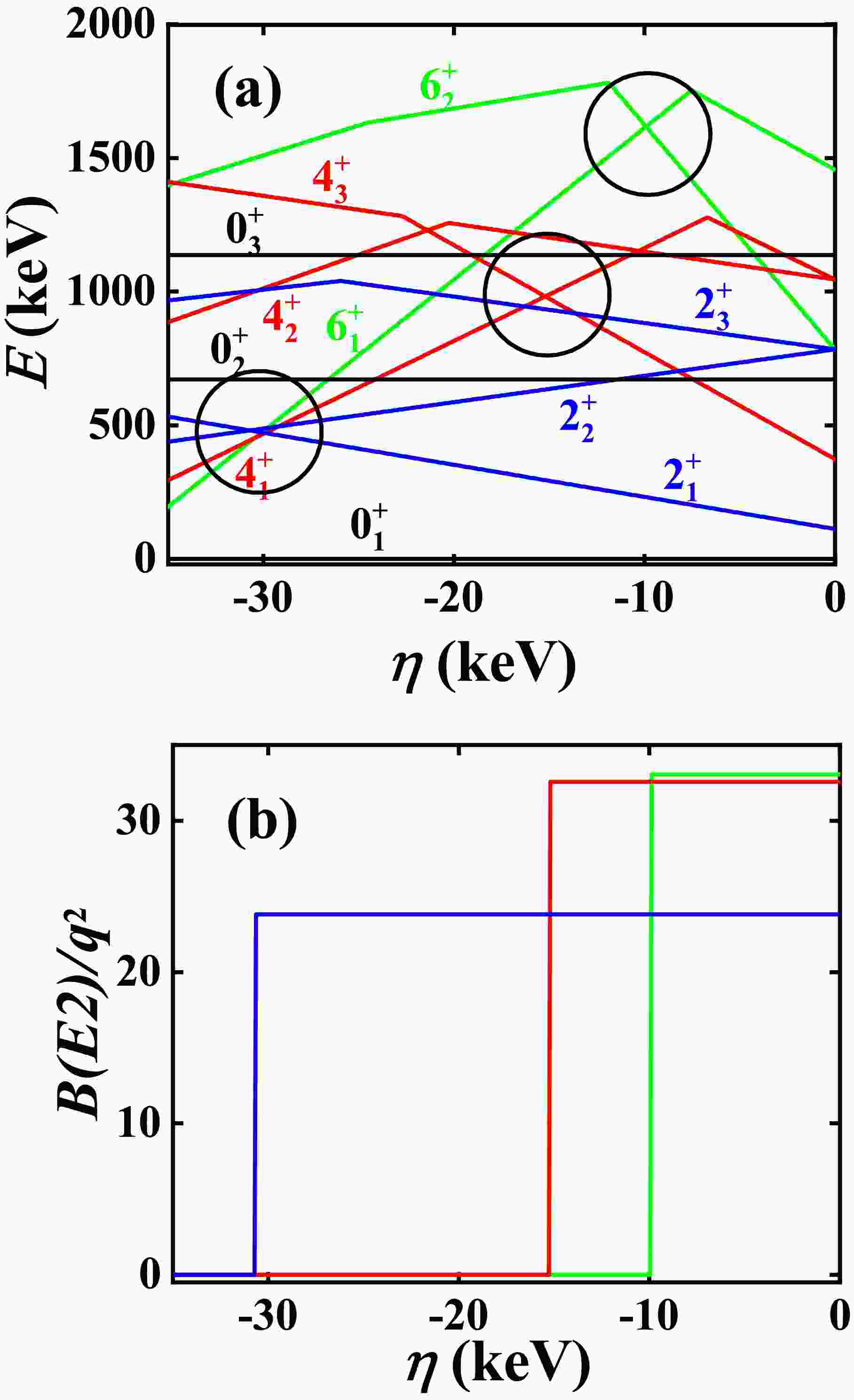For the SU(3) symmetry limit part, let the parameter η in front of the third-order interaction $ [\hat{L} \times \hat{Q} \times \hat{L}]^{(0)} $ change gradually, and observe whether the $ 4_{1}^{+} $ state can intersect with another higher $ 4^{+} $ state and whether other level-crossing phenomena can appear.

Fig. 1(a) shows the evolutionary behaviors of the low-lying $ 0^{+} $, $ 2^{+} $, $ 4^{+} $, and $ 6^{+} $ states when the parameter η decreases from 0. We can observe that the first $ 4^{+} $ state crosses over with another higher $ 4^{+} $ state at $ \eta=-15.20 $ keV (solid red lines and black circle). Before this crossover point, the $ 6_{1}^{+} $ state first intersects with another higher $ 6^{+} $ state at $ \eta=-10.04 $ keV (solid green lines and black circle). When η further decreases, the first $ 2^{+} $ state also crosses over with another higher $ 2^{+} $ state at $ \eta=-30.72 $ keV (solid blue lines and black circle). In the SU(3) symmetry limit, if two levels belong to two different SU(3) irreps $ (\lambda, \mu) $, the B(E2) transitions between the two levels must be zero. After the crossover point of the two $ 4^{+} $ states and before the crossover point of the two $ 2^{+} $ states (from $ - $15.20 keV to $ - $30.72 keV), a B(E2) anomaly exists because the $ B_{4/2} $ value is 0.

Figure 1.  (color online) (a) The evolutionary behaviors of the partial low-lying levels as a function of η; (b) The evolutionary behaviors of the $ B(E2; 2_{1}^{+}\rightarrow 0_{1}^{+}) $ (blue line), $ B(E2; 4_{1}^{+}\rightarrow 2_{1}^{+}) $ (red line), and $ B(E2; 6_{1}^{+}\rightarrow 4_{1}^{+}) $ (green line) as a function of η. The parameters are deduced from [40].

The $ B_{4/2} $ values in the U(5) symmetry limit and the O(6) symmetry limit are both normal [42], with $ B_{4/2}>1.0 $. Thus if $ B_{4/2}=0 $ in the SU(3) symmetry limit, a realistic $ B_{4/2}<1.0 $ value can be obtained when moving towards the U(5) symmetry limit or the O(6) symmetry limit. However, the two recovery mechanisms are very different. In Fig. 1, the crossover of the $ 4_{1}^{+} $ state and another higher $ 4^{+} $ state induces the B(E2) anomaly. Thus, when moving towards the U(5) symmetry limit, the two $ 4^{+} $ states exhibit a level-anticrossing phenomenon, unwinding the crossover in the SU(3) symmetry limit.

However, when moving towards the O(6) symmetry limit, the unwinding phenomenon cannot occur [51]. Fig. 2 shows the evolutionary behaviors from the SU(3) symmetry limit to the O(6) symmetry limit when $ \eta=-20.0 $ keV (here the parameter changes from $ -\dfrac{\sqrt{7}}{2} $ to $ -0.7 $). Clearly, the evolutionary behaviors of the two $ 4_{1}^{+} $ and $ 4_{2}^{+} $ states do not exhibit level-anticrossing. Instead, the B(E2) anomaly results from the level-anticrossing of the two $ 2_{1}^{+} $ and $ 2_{2}^{+} $ states (solid blue lines and black circle).

Figure 2.  (color online) (a) The evolutionary behaviors of the partial low-lying levels as a function of χ; (b) The evolutionary behaviors of the $ B(E2; 2_{1}^{+}\rightarrow 0_{1}^{+}) $ (blue line), $ B(E2; 4_{1}^{+}\rightarrow 2_{1}^{+}) $ (red line), and $ B(E2; 6_{1}^{+}\rightarrow 4_{1}^{+}) $ (green line) as a function of χ. The parameters are deduced from [40].

In [44], it was found that, even if the $ B_{4/2} $ value is larger than 1.0 in the SU(3) symmetry limit (here $ \eta>15.20 $ keV), when moving towards the O(6) symmetry limit, the B(E2) anomaly can also occur. Fig. 3 shows the evolutionary behaviors from the SU(3) symmetry limit to the O(6) symmetry limit when $ \eta=-10.0 $ keV. Clearly, in the SU(3) symmetry limit, the $ B_{4/2} $ value is normal. When χ increases, the $ 6_{1}^{+} $ and $ 6_{2}^{+} $ states first exhibit level-anticrossing (solid green lines and black circle), followed by the $ 4_{1}^{+} $ and $ 4_{2}^{+} $ states (solid red lines and black circle), and lastly the $ 2_{1}^{+} $ and $ 2_{2}^{+} $ states (solid blue lines and black circle). Thus, the B(E2) anomaly can occur. This new mechanism has been incorporated into the previous level-crossing mechanism, and a general explanatory framework has been obtained. A detailed discussion can be seen in [51].

Figure 3.  (color online) (a) The evolutionary behaviors of the partial low-lying levels as a function of χ; (b) The evolutionary behaviors of the $ B(E2; 2_{1}^{+}\rightarrow 0_{1}^{+}) $ (blue line), $ B(E2; 4_{1}^{+}\rightarrow 2_{1}^{+}) $ (red line), and $ B(E2; 6_{1}^{+}\rightarrow 4_{1}^{+}) $ (green line) as a function of χ. The parameters are deduced from [40].

The three different mechanisms discussed here will be used to fit the $ B(E2;2^{+}_{1}\rightarrow0^{+}_{1}) $ anomaly in $ ^{166} {\rm{Os}}$ and the B(E2) anomalies in $ ^{168,170} {\rm{Os}}$ simultaneously.

In Fig. 4, the evolutionary behavior of the $B(E2;2_{1}^{+}\rightarrow0_{1}^{+}$) values in $^{166-170}{\rm{ Os}}$ is shown. When the boson number decreases from 9 to 7, the value decreases from 97(9) W.u., normally to 74(13) W.u., and then, suddenly, to 7(4) W.u. The $B(E2;2^{+}_{1}\rightarrow0^{+}_{1})$ value in $^{166}{\rm{ Os}}$ is almost 10 times smaller than the one in $^{168}{\rm{ Os}}$ while the boson number is only one less. Such a very small $B(E2;2^{+}_{1}\rightarrow0^{+}_{1})$ value, typically, can only occur in magic nuclei. When moving away from the magic nuclei, this value increases significantly. If $N\geq5$, the nucleus can have a deformed shape, and the $B(E2;2^{+}_{1}\rightarrow0^{+}_{1})$ value is large. The two adjacent nuclei $^{168,170}{\rm{ Os}}$ indeed follow this pattern. Similar evolutionary behavior can also be observed in $^{162-166}{\rm{ W}}$. The $B(E2;2^{+}_{1}\rightarrow0^{+}_{1})$ value in $^{162}{\rm{ W}}$ is 31(13) W.u. [69], which is almost 5 times smaller than the value 150(100) W.u. in $^{164}{\rm{ W}}$ [69].

Figure 4.  (color online) Experimental $ B(E2;2_{1}^{+}\rightarrow0_{1}^{+}) $ values in $ ^{162-166} {\rm{W}}$ and $ ^{166-170} {\rm{Os}}$ as a function of the boson number N. These values are from [36−38, 68, 69].

In Table 1, the $B(E2;2_{1}^{+}\rightarrow0_{1}^{+}$) values of 22 nuclei with $N=7$ are shown. From the top, the three nuclei $^{146}{\rm{ Gd}}$, $^{118}{\rm{ Sn}}$, and $^{114}{\rm{ Sn}}$ in the first group are magic nuclei (proton or neutron boson number is 0). The $B(E2;2_{1}^{+}\rightarrow0_{1}^{+}$) values are small, but the values in $^{114,118}{\rm{ Sn}}$ are still larger than the one in $^{166}{\rm{ Os}}$. The proton or neutron boson number of the five nuclei in the second group is 1, and the average value of the five nuclei is 34.0 W.u., much larger than those of the magic nuclei in the first group. Next, the proton or neutron boson number of the six nuclei in the third group is 2, and the average value is 46.6 W.u., larger than that of the nuclei in the second group.

nucleus	$B(E2;2^{+}_{1}\rightarrow0^{+}_{1})$	nucleus	$B(E2;2^{+}_{1}\rightarrow0^{+}_{1})$
$^{146}{\rm{ Gd}}$	$>$ 0.59	$^{118}{\rm{ Sn}}$	12.1(5)
$^{114}{\rm{ Sn}}$	15(3)
$^{194}{\rm{ Hg}}$	$39^{+9}_{-6}$	$^{122}{\rm{ Te}}$	36.92(25)
$^{118}{\rm{ Cd}}$	33(3)	$^{114}{\rm{ Te}}$	34.0(30)
$^{110}{\rm{ Cd}}$	27.0(8)
$^{194}{\rm{ Pt}}$	49.5(20)	$^{146}{\rm{ Nd}}$	31.9(4)
$^{138}{\rm{ Nd}}$	36(1)	$^{126}{\rm{ Xe}}$	56(5)
$^{114}{\rm{ Xe}}$	62(4)	$^{106}{\rm{ Pd}}$	44.3(15)
$^{194}{\rm{ Os}}$	45(16)	$^{166}{\rm{ Os}}$	7(4)
$^{162}{\rm{ W}}$	31(13)	$^{146}{\rm{ Ce}}$	43(5)
$^{146}{\rm{ Ba}}$	59.7(19)	$^{134}{\rm{ Ce}}$	50.8(41)
$^{130}{\rm{ Ba}}$	57.9(17)	$^{102}{\rm{ Ru}}$	44.6 (7)

Table 1.  $B(E2;2^{+}_{1}\rightarrow0^{+}_{1})$ values of 22 nuclei with $N=7$. The unit is W.u. These values are from [34, 35, 68−75].

Lastly, the proton or neutron boson number of the eight nuclei in the fourth group is 3, and the average value, except for $^{166}{\rm{ Os}}$ and $^{162}{\rm{ W}}$, is 50.2 W.u., larger than that of the nuclei in the third group. This is the normal trend. If $^{166}{\rm{ Os}}$ and $^{162}{\rm{ W}}$ are included, the average value is 38.6 W.u., smaller than the 46.6 W.u. in the third group. The normal average value of 50.2 W.u. can also be deduced from Fig. 1 with normal extrapolation. The $B(E2;2_{1}^{+}\rightarrow0_{1}^{+}$) value in $^{166}{\rm{ Os}}$ is very small, almost 7 times smaller than this normal average value, which is an anomalous phenomenon.

Through the above discussions, the $B(E2;2_{1}^{+}\rightarrow0_{1}^{+}$) anomaly in $^{166}{\rm{ Os}}$ really exists.

In [51], a general explanatory framework for the B(E2) anomaly was proposed based on the SU(3) analysis up to the SU(3) third-order interactions. The Hamiltonian is as follows:

where $\varepsilon_{d}$, κ, ζ, η, and f are five fitting parameters. $\hat{n}_{d}=d^{\dagger} \cdot \tilde{d}$ is the d boson number operator, and $\hat{Q}_{\chi}= (d^{\dagger}s + s^{\dagger}\tilde{d}) + \chi(d^{\dagger} \times \tilde{d})$ is the general quadrupole operator ($-\dfrac{\sqrt{7}}{2} \leq \chi \leq 0$). If $\varepsilon_{d}=0$ and $\chi=-\dfrac{\sqrt{7}}{2}$, this Hamiltonian corresponds to the SU(3) analysis. The $-\hat{Q}\cdot \hat{Q}$ interaction can describe the prolate shape, and the $-[\hat{Q} \times \hat{Q} \times \hat{Q}]^{(0)}$ interaction can describe the oblate shape [59]. The third-order interaction $[\hat{L} \times \hat{Q} \times \hat{L}]^{(0)}$ is vital for the emergence of the B(E2) anomaly.

For understanding the B(E2) anomaly, the B(E2) values are necessary. The $E2$ operator is defined as

where q is the boson effective charge. The evolutionary behaviors of the $B(E2;4_{1}^{+}\rightarrow2_{1}^{+})$ and $B(E2;2_{1}^{+}\rightarrow0_{1}^{+})$ values are discussed. Here $q=Nq_{0}$ is used. When discussing higher-order interactions, the simple form in (2) is usually used [76−78]. If more accurate results are desired, the higher-order interaction $[\hat{Q}_{\chi} \times \hat{Q}_{\chi}]^{(2)}$ should be considered [2, 27]. In the existing discussions with the SU3-IBM, we found that the simple form in (2) is sufficiently accurate [57, 62].

One may doubt whether the boson number N used here is applicable. In a recent paper on the boson number odd-even effect in $^{196-204}{\rm{ Hg}}$ [63], it was proven that the boson number N must be the valence nucleon-pair number, which validates the boson number assumption in the IBM.

Following the ideas in Section II, we perform the SU(3) analysis for $N=7, 8, 9$. In Fig. 5, the evolutional behaviors of the $B(E2;2_{1}^{+}\rightarrow 0_{1}^{+})$ values (solid lines) and $B(E2;4_{1}^{+}\rightarrow2_{1}^{+})$ values (dashed lines) as a function of η are presented. Other parameters are $\varepsilon_{d}=0$ keV, $\chi=-\dfrac{\sqrt{7}}{2}$, $\kappa=30.09$ keV, $\zeta=3.79$ keV, and $f=18.66$ keV [18]. The boson numbers N are 7 for $^{166}{\rm{ Os}}$ (black lines), 8 for $^{168}{\rm{ Os}}$ (red lines), and 9 for $^{170}{\rm{ Os}}$ (blue lines), respectively. The SU(3) irrep of the ground state is $(2N,0)$, which corresponds to the prolate shape. Thus, the B(E2) values are the largest among all the SU(3) irreps $(\lambda,\mu)$.

Figure 5.  (color online) The evolutionary behaviors of the $B(E2;2_{1}^{+}\rightarrow0_{1}^{+})$ (solid lines) and $B(E2;4_{1}^{+}\rightarrow2_{1}^{+})$ (dashed lines) values are shown as a function of η for $N=9$ (blue lines), $N=8$ (red lines), and $N=7$ (black lines). The parameters are derived from [40].

For different N, the parameters η for the emergence of $B(E2;4_{1}^{+}\rightarrow 2_{1}^{+})=0$ and $B(E2;2_{1}^{+}\rightarrow 0_{1}^{+})=0$ are different, and if N decreases, the parameters decrease as well.

The validity of the parameter setting of the effective charge $q=Nq_{0}$ requires explanation here. Under normal circumstances, the $B(E2;2_{1}^{+}\rightarrow 0_{1}^{+})$ value in $^{166}{\rm{ Os}}$ should be around 50.2 W.u. (the normal average value discussed in Section III). The $B(E2;2_{1}^{+}\rightarrow 0_{1}^{+})$ values in $^{168,170}{\rm{ Os}}$ are 74(13) W.u. and 97(9) W.u., respectively. Thus, the normal ratio for $^{166-170}{\rm{ Os}}$ is 50.2:74:97. In Fig. 5, the SU(3) analysis gives the ratio of the $B(E2;2_{1}^{+}\rightarrow 0_{1}^{+})$ values for $N=7,8,9$ as 23.8:30.4:37.8, or 61:78:97. If q is the same for $^{166-170}{\rm{ Os}}$, the experimental data cannot be obtained. If $q=Nq_{0}$, the ratio of the $B(E2;2_{1}^{+}\rightarrow 0_{1}^{+})$ values for $^{166-170}{\rm{ Os}}$ is $61\times7^{2}:78\times8^{2}:97\times9^{2}$ or 36.9:61.6:97. When the $\hat{n}_{d}$ interaction is added or the parameter χ changes from $-\dfrac{\sqrt{7}}{2}$ to 0, the normal ratio 50.2:74:97 can be obtained. Thus, the setting $q=Nq_{0}$ is reasonable, and the very small $B(E2;2_{1}^{+}\rightarrow 0_{1}^{+})$ value in $^{166}{\rm{ Os}}$ results from level-crossing.

Now, we fit the isotopes $^{166,168,170}{\rm{ Os}}$ based on the results in Fig. 5. In this paper, we present four results for $^{166-170}{\rm{ Os}}$ from the three different mechanisms shown in section II. Table 2 presents the fitting parameters for these four results.

Res. 1	χ	$\varepsilon_{d} $	κ	ζ	η	f
$^{170}{\rm{ Os}}$	$-\sqrt{7}/2$	306	30.09	3.79	$-10.38$	18.66
$^{168}{\rm{ Os}}$	$-\sqrt{7}/2$	328	31.72	3.99	$-14.69$	19.67
$^{166}{\rm{ Os}}$	$-\sqrt{7}/2$	31.2	10.76	1.36	$-11.92$	50.20
Res. 2	χ	$\varepsilon_{d} $	κ	ζ	η	f
$^{170}{\rm{ Os}}$	$-1.1192$	0	30.27	$-5.01$	$-8.91$	27.79
$^{168}{\rm{ Os}}$	$-1.0266$	0	30.27	$-5.01$	$-12.01$	33.64
$^{166}{\rm{ Os}}$	$-1.3044$	0	21.70	$-3.59$	$-13.88$	41.57
Res. 3	χ	$\varepsilon_{d} $	κ	ζ	η	f
$^{170}{\rm{ Os}}$	$-1.0583$	0	79.31	$-13.13$	$-16.13$	5.06
$^{168}{\rm{ Os}}$	$-0.9551$	0	85.64	$-14.18$	$-21.63$	2.77
$^{166}{\rm{ Os}}$	$-1.0504$	0	29.26	$-4.84$	$-18.46$	45.77
Res. 4	χ	$\varepsilon_{d} $	κ	ζ	η	f
$^{170}{\rm{ Os}}$	$-1.1562$	0	120.69	$-19.99$	$-24.54$	$-21.49$
$^{168}{\rm{ Os}}$	$-1.1324$	0	97.67	$-16.17$	$-26.71$	$-11.74$
$^{166}{\rm{ Os}}$	$-1.1192$	0	25.52	$-4.23$	$-15.70$	42.84

Table 2.  The fitting parameters for the four results of $^{166,168,170}{\rm{ Os}}$ are presented. The unit is keV, except for χ.

The concept of fitting for any result is as follows. We first fit the B(E2) anomaly in $^{170}{\rm{ Os}}$, for which a significant amount of experimental data has been accumulated. Based on the results (indicated by blue lines) in Fig. 5, the parameter η is determined. Then, the $\hat{n}_{d}$ interaction is added, or the parameter χ is adjusted from $-\dfrac{\sqrt{7}}{2}$ to 0. The $B_{4/2}$ value that matches the experimental one in $^{170}{\rm{ Os}}$ can be found. To make the energy of the $2_{1}^{+}$ state equal to the experimental value, all parameters should be multiplied by the same factor, allowing the parameters to be accurately determined, as shown in Table 2. When the $B_{4/2}$ value in $^{170}{\rm{ Os}}$ is set equal to the experimental one, the parameter $q_{0}$ can be determined, and subsequently, the effective charge q is obtained. For each result, the parameter $q_{0}$ remains consistent. This ensures that the variation in the effective charge q is not too significant for $^{168-170}{\rm{ Os}}$ and aligns with the actual observations. Using a similar method, the parameters for $^{168}{\rm{ Os}}$ and $^{166}{\rm{ Os}}$ can be determined successively.

For Result 1, the $\hat{n}_{d}$ interaction is added (the first mechanism). $^{168,170}{\rm{ Os}}$ exhibits a B(E2) anomaly. The parameter η is chosen from the region satisfying $B(E2;2^{+}_{1}\rightarrow0^{+}_{1})\neq0$ and $B(E2;4^{+}_{1}\rightarrow2^{+}_{1})=0$. For $^{166}{\rm{ Os}}$, the $B(E2;2^{+}_{1}\rightarrow0^{+}_{1})$ value is very small, so the parameter η is determined from the region satisfying $B(E2;2^{+}_{1}\rightarrow0^{+}_{1})=0$ and $B(E2;4^{+}_{1}\rightarrow2^{+}_{1})=0$. This possibility is unique if the results are obtained by adding the $\hat{n}_{d}$ interaction.

It should be noted that the choice of the parameters is fairly robust. The fitting values of result 1 for $^{166-170}{\rm{ Os}}$ can be seen in Table 3 (the energies of the $2_{1}^{+}$, $4_{1}^{+}$, $6_{1}^{+}$, and $8_{1}^{+}$ states) and Table 4 (the values of the E2 transitions $B(E2;2_{1}^{+}\rightarrow0_{1}^{+})$, $B(E2;4_{1}^{+}\rightarrow2_{1}^{+})$, $B(E2;6_{1}^{+}\rightarrow4_{1}^{+})$, $B(E2;8_{1}^{+}\rightarrow 6_{1}^{+})$). The B(E2) values agree with the experimental ones.

$^{170}{\rm{ Os}}$	Exp.	Res. 1	Res. 2	Res. 3	Res. 4
$E_{2_{1}^{+}}$	286.70(14)	283.73	287.27	287.05	286.99
$E_{4_{1}^{+}}$	749.90(20)	733.19	749.99	759.98	900.84
$E_{6_{1}^{+}}$	1325.42(24)	1237.10	1476.23	1422.26	1245.82
$E_{8_{1}^{+}}$	1946.8(4)	1960.00	2557.86	2413.02	2620.62
$^{168}{\rm{ Os}}$	Exp.	Res. 1	Res. 2	Res. 3	Res. 4
$E_{2_{1}^{+}}$	341.20(20)	342.81	343.07	341.92	342.15
$E_{4_{1}^{+}}$	857.3(3)	973.07	867.36	848.99	1085.14
$E_{6_{1}^{+}}$	1499.1(4)	1548.01	1697.49	1510.92	1500.22
$E_{8_{1}^{+}}$	2222.7(4)	2429.90	2987.13	2537.08	2225.40
$^{166}{\rm{ Os}}$	Exp.	Res. 1	Res. 2	Res. 3	Res. 4
$E_{2_{1}^{+}}$	432.0(3)	432.03	428.26	439.94	429.40
$E_{4_{1}^{+}}$	1021.0(5)	1020.22	1010.74	1046.30	1019.02
$E_{6_{1}^{+}}$	1725.0(7)	1974.57	1948.34	2073.91	1989.63
$E_{8_{1}^{+}}$	2351.3(9)	3653.00	3575.69	3873.44	3663.40

Table 3.  Experimental energy values and fitted data of the four results for certain states along the yrast band for $^{166-170}{\rm{ Os}}$. The unit is keV.

$^{170}{\rm{ Os}}$	Exp.	Res. 1	Res. 2	Res. 3	Res. 4
$B(E2;2^{+}_{1}\rightarrow0^{+}_{1})$	97(9)	96.30	97.05	96.99	97.01
$B(E2;4^{+}_{1}\rightarrow2^{+}_{1})$	38 $^{+18}_{-7}$	37.83	37.79	38.28	38.20
$B(E2;6^{+}_{1}\rightarrow4^{+}_{1})$		33.70	42.50	41.08	13.96
$B(E2;8^{+}_{1}\rightarrow6^{+}_{1})$		21.96	34.18	33.71	15.55
${ B}_{4/2}$	0.39	0.39	0.39	0.40	0.39
$^{168}{\rm{ Os}}$	Exp.	Res. 1	Res. 2	Res. 3	Res. 4
$B(E2;2^{+}_{1}\rightarrow0^{+}_{1})$	74(13)	74.97	76.36	74.03	62.55
$B(E2;4^{+}_{1}\rightarrow2^{+}_{1})$	25(13)	25.35	25.44	25.16	21.67
$B(E2;6^{+}_{1}\rightarrow4^{+}_{1})$		17.64	28.24	26.43	5.84
$B(E2;8^{+}_{1}\rightarrow6^{+}_{1})$		11.15	21.85	20.62	6.19
${ B}_{4/2}$	0.338	0.340	0.333	0.340	0.346
$^{166}{\rm{ Os}}$	Exp.	Res. 1	Res. 2	Res. 3	Res. 4
$B(E2;2^{+}_{1}\rightarrow0^{+}_{1})$	7(2)	7.24	7.29	7.01	7.10
$B(E2;4^{+}_{1}\rightarrow2^{+}_{1})$		0.33	0.04	3.33	1.10
$B(E2;6^{+}_{1}\rightarrow4^{+}_{1})$		0.38	0.10	3.70	1.59
$B(E2;8^{+}_{1}\rightarrow6^{+}_{1})$	1.4(5)	1.01	2.08	2.83	1.43
${B}_{8/2}$	0.20	0.14	0.29	0.40	0.20

Table 4.  Experimental B(E2) values and fitted data for the four results are presented for the $B(E2;2^{+}_{1}\rightarrow0^{+}_{1})$, $B(E2;4^{+}_{1}\rightarrow2^{+}_{1})$, $B(E2;6^{+}_{1}\rightarrow4^{+}_{1})$, and $B(E2;8^{+}_{1}\rightarrow6^{+}_{1})$ transitions for $^{166-170}{\rm{ Os}}$. The unit is W.u. For results $1-4$ of $^{170}{\rm{ Os}}$, the $q_{0}$ values are 0.0166054 eb, 0.0268821 eb, 0.0169294 eb, and 0.0135674 eb, respectively.

The ground band, β band, and γ band of the fitted levels for $^{166}{\rm{ Os}}$ can be seen in Fig. 6. Some other fitted B(E2) values for $^{166}{\rm{ Os}}$ are listed in Table 5. It is expected that these results can be further compared in future experiments.

Figure 6.  The ground band, β band, and γ band of the fitted levels for ¹⁶⁶Os are shown in results 1−4.

$^{166}{\rm{ Os}}$	Res. 1	Res. 2	Res. 3	Res. 4
$B(E2;2^{+}_{1}\rightarrow0^{+}_{2})$	2.98	7.96	4.09	2.03
$B(E2;2^{+}_{2}\rightarrow0^{+}_{2})$	0.65	0.45	1.52	0.89
$B(E2;2^{+}_{2}\rightarrow2^{+}_{1})$	24.47	31.64	18.77	22.28
$B(E2;2^{+}_{3}\rightarrow2^{+}_{1})$	0.0	0.01	0.43	0.14
$B(E2;3^{+}_{1}\rightarrow2^{+}_{1})$	52.63	157.28	48.00	30.62
$B(E2;4^{+}_{1}\rightarrow3^{+}_{1})$	0.01	0.0	0.18	0.04
$B(E2;4^{+}_{1}\rightarrow2^{+}_{2})$	0.03	0.01	0.12	0.13
$B(E2;4^{+}_{1}\rightarrow2^{+}_{3})$	0.0	14.55	5.85	3.91
$B(E2;4^{+}_{3}\rightarrow4^{+}_{1})$	0.0	0.01	0.42	0.22
$B(E2;5^{+}_{1}\rightarrow4^{+}_{1})$	30.31	81.98	26.12	18.04

Table 5.  Fitted data of some other B(E2) values for $^{166}{\rm{ Os}}$. The unit is W.u. The parameter $q_{0}$ is the same as the one in Table IV.

For $^{166}{\rm{ Os}}$, not only the $B(E2;2_{1}^{+}\rightarrow0_{1}^{+})$ value but also the $B(E2;8_{1}^{+}\rightarrow6_{1}^{+})$ value has been measured. The experimental $B(E2;8_{1}^{+}\rightarrow6_{1}^{+})$ value is 1.4(5) W.u., and the theoretical value is 1.01 W.u. Thus, the fitting effect of result 1 is good.

Ref. [40] proposed the SU3-IBM and described the B(E2) anomaly in $^{170}{\rm{ Os}}$, which provided a new understanding of nuclear structure. Now, we show that this mechanism can still describe the B(E2) anomaly in $^{168,170}{\rm{ Os}}$ and the $B(E2;2_{1}^{+}\rightarrow0_{1}^{+})$ anomaly in $^{166}{\rm{ Os}}$ simultaneously. Thus, the level-crossing explanation is useful.

For results $2-4$, we set $\varepsilon_{d} = 0$ and slightly adjust χ, as proposed by [44]. For result 2, we also select the parameter η for fitting $^{166-170}{\rm{ Os}}$ in the anomalous region of Fig. 5 (the second mechanism in Fig. 2). From Table 3 and Table 4, the fitting effect of result 2 is notable except that the $B(E2;8_{1}^{+}\rightarrow6_{1}^{+})$ value in $^{166}{\rm{ Os}}$ is somewhat larger. The $B(E2;4_{1}^{+}\rightarrow2_{1}^{+})$ and $B(E2;6_{1}^{+}\rightarrow4_{1}^{+})$ values in $^{166}{\rm{ Os}}$ are smaller than those in result 1.

When the parameter χ changes from $-\dfrac{\sqrt{7}}{2}$ to 0, Ref. [44] found new possibilities. If the $B_{4/2}$ value is larger than 1.0 in the SU(3) analysis, as χ changes, the B(E2) anomaly can also be observed (the third mechanism in Fig. 3). This has been discussed in detail in [44, 51]. Level-anticrossing of the $4_{1}^{+}$ state and another $4^{+}$ state can occur. Thus, different from results 1 and 2, in this case, there are two parameter points satisfying the experimental data in $^{170}{\rm{ Os}}$, leading to results 3 and 4.

Result 3 chooses the $B_{4/2}$ value towards the O(6) side in $^{170}{\rm{ Os}}$. From Table 3 and Table 4, the fit remains good except that the $B(E2;8_{1}^{+}\rightarrow6_{1}^{+})$ value in $^{166}{\rm{ Os}}$ is much larger than those in Results 1 and 2. The $B(E2;4_{1}^{+}\rightarrow2_{1}^{+})$ and $B(E2;6_{1}^{+}\rightarrow4_{1}^{+})$ values in $^{166}{\rm{ Os}}$ are significantly larger than those in Results 1 and 2.

Result 4 chooses the $B_{4/2}$ value towards the SU(3) side in $^{170}{\rm{ Os}}$. This possibility was pointed out in [51]. From Table 3 and Table 4, the fit remains good. The $B(E2;4_{1}^{+}\rightarrow2_{1}^{+})$ and $B(E2;6_{1}^{+}\rightarrow4_{1}^{+})$ values in $^{168,170}{\rm{ Os}}$ are also larger than those in Results 1 and 2.

Thus, the four results provide different predictions for the $B(E2;4_{1}^{+}\rightarrow2_{1}^{+})$ and $B(E2;6_{1}^{+}\rightarrow4_{1}^{+})$ values in $^{166}{\rm{ Os}}$, which future experiments can verify.

For Hamiltonian (1), only the third-order interactions are considered, and the fourth-order interactions are not added. The reason for this is that the functions of these fourth-order interactions on the B(E2) anomaly are not discussed clearly because the effects may be very complicated, and detailed studies are needed in future. In [56], it was found that the fourth-order interactions can affect the positions of the levels greatly, but the B(E2) values slightly. When discussing the Cd nuclei, the fourth-order interactions can make the energy levels fit well. In a recent paper on $^{106}{\rm{ Pd}}$ [57], this result can be also obtained. Thus in following studies, the introduction of the fourth-order interactions may make the energy levels in Table 3 fit better, especially the $8_{1}^{+}$ state.

It should be stressed that the small $B(E2;8_{1}^{+}\rightarrow6_{1}^{+})$ value is not an accident result. In the level-crossing explanation, when $[\hat{L} \times \hat{Q} \times \hat{L}]^{(0)}$ decreases, the $B(E2;8_{1}^{+}\rightarrow6_{1}^{+})$ anomaly first occurs, and then $B(E2;6_{1}^{+}\rightarrow4_{1}^{+})$ anomaly, $B(E2;4_{1}^{+}\rightarrow2_{1}^{+})$ anomaly and $B(E2;2_{1}^{+}\rightarrow0_{1}^{+})$ anomaly. Thus the small $B(E2;2_{1}^{+}\rightarrow0_{1}^{+})$ value implies the emergence of the small $B(E2;8_{1}^{+}\rightarrow6_{1}^{+})$ value, and our fits prove this result.

In [68], the very small $B(E2;8_{1}^{+}\rightarrow6_{1}^{+})$ value results from band-crossing, which is an interesting phenomenon to be further discussed. The B(E2) value of $B(E2;8_{2}^{+}\rightarrow6_{1}^{+})$ need to be measured, and the $8_{2}^{+}$ state may belong to the ground band.

In this paper, we show that the level-crossing mechanism or the general explanatory framework really explain the $B(E2;2_{1}^{+}\rightarrow0_{1}^{+})$ anomaly in $^{166}{\rm{ Os}}$. However the best fitting conditions are not discussed, because the fourth-order interaction effects are not clear. In Table 2, the fitting parameters for $^{166-170}{\rm{ Os}}$ are not so natural, and change abruptly, so a better fitting effect is needed. This will be discussed in next paper.

This paper employs the SU(3) analysis technique to comparatively analyze the three mechanisms that cause the B(E2) anomaly to explain the very small $B(E2;2_{1}^{+}\rightarrow0_{1}^{+})$ anomaly in $^{166}{\rm{ Os}}$. Appropriate parameters are selected to fit the $^{166,168,170}{\rm{ Os}}$. The fitting results closely approximate the experimental data. Not only the B(E2) anomaly in $^{168,170}{\rm{ Os}}$ but also the $B(E2;2_{1}^{+}\rightarrow0_{1}^{+})$ anomaly in $^{166}{\rm{ Os}}$ are described simultaneously. This implies that the level-crossing or level-anticrossing mechanism is necessary for understanding the B(E2) anomaly. There are many possible mechanisms for describing the B(E2) anomaly, here we show that the general explanatory framework in [51] is really useful.