Neutron stars and Pulsar timing arrays as Axion giant gyroscopes

Oscillating background fields across the cosmic space, which behave like matter, are interesting dark matter candidates [1−5]. The most common ones are either axionlike pseudoscalars or scalar fields such as moduli [6−9]. Since axion has a large parameter space, various axion detection schemes are proposed across the spectrum ¹, from the quantum laboratory and collider studies to astrophysical observations. Inspired by the nucleon spin precession detection of axion particles such as CASPEr [10], here we extend the detection principle using the microscopic nucleon spins to the macroscopic neutron stars, such that the three-dimensional rotating motion of spinning neutron stars blown by the axion wind can yield signals for an extensive range of parameter space for the axion mass and decay constant. The current constraints on using PTA systems with neutron stars to detect axions have recently attracted research attention [11−19]. The previous study mainly focused on the axion cloud halos' modulation effects on the electromagnetic signals. Here in this paper, we mostly discuss the case where ultralight axion wind blows on the pulsars in PTA. And this wind blows causes the change of the pulsar's period, which yields the common spectrum on the residual with $ f_c =\dfrac{\omega}{2\pi}\simeq 2.42 \text{ nHz} \left(\dfrac{m}{10^{-23}\text{eV}} \right) $ and two-point correlation function curve. We also briefly comment on the modulation of the pulsar period with different axion masses e.g.QCD axion $ 242 \text{ MHz} \left(\dfrac{m}{10^{-6}\text{eV}} \right) $, or the resonant frequency with pulsar period $ 2.42 \text{ kHz} \left(\dfrac{m}{10^{-11}\text{eV}} \right) $.

Recently several Pulsar Timing Arrays (PTAs) observatories including NANOGrav(North American Nanohertz Observatory for Gravitational Waves) [20], Parkes PTA (PPTA) [21], European PTA (EPTA) [22, 23] and Chinese PTA (CPTA) [24], report strong evidence for gravitational wave (GW) background at the nano-Hertz waveband, which is consistent with previous claims [25−28]. Extensive studies on potential sources of the observed GW background [29−57], including supermassive black holes [58−61], merging PBHs [62, 63], phase transitions [64−67] and axion topological defects [14, 68, 69], etc are conducted. Nongravitational wave signals, such as the ultralight dark matter can also be observed through the timing residuals [38, 70−75].

Most of the pulsars we observed are at the distances of order kpc from the Earth. The de Broglie wavelength of the ultralight dark matter is around $ \lambda_{\text {dB}}=\dfrac{2\pi}{{m} v} \simeq 4 \text{kpc} \left(\dfrac{10^{-23}\text{eV}}{m}\right) \left(\dfrac{10^{-3}}{v}\right) $. Fuzzy dark matter oscillates with the frequency $ 2.42 \text{ nHz} \left(\dfrac{m}{10^{-23}\text{eV}} \right) $ and the oscillation period $ T_c={f}_c^{-1} \simeq 13.1 \text{yr} \left(\dfrac{10^{-23}\text{eV}}{m}\right) $. The field behaves like pressureless cold dark matter on the cosmic scale. Notably, the oscillation frequencies of fuzzy dark matter models fell into the sensitive region of PTA observations.

Uncertainties exist in the dark matter wave model in this work. For instance, primordial axion dark matter may initially exhibit coherence, but then may undergo fragmentation upon infall into galactic halos. Nevertheless, it might still reorganize into a wave-like state, such as forming a Bose-Einstein condensate (BEC)[76, 77]. Taking into account the huge occupation number of the dark matter particle in the universe, the axion field in the Galaxy can be viewed as a classical field and approximated by[70, 78−92]

where $ m_a $ is the mass of the axion, v is the typical velocity of the axion and $ \rho_{DM}\sim0.3 \mathrm{GeV/cm^3} $ is the local dark matter density. The macroscopic behaviour of axions has a classical description, best obtained by computing the coherent state of its quantum field—any quantum fluctuations in such a highly occupied system will be negligible. According to the literature, this well justified the classical plane wave approximation we used. The Hamiltonian of the interaction between the axion and the nucleon is given by[93, 94]

where $ g_{aNN} $ is the coulping constant and $ \vec{\sigma} $ is the nuclear-spin operator.

As it is known that the magnetic moment $ \vec{\mu} $ can be expressed in terms of the nuclear spin $ \vec{\sigma} $

where γ is the gyromagnetic ratio of the nuclear spin, related to the property of the nucleon. Define the effective magnetic field induced by the axion[95]:

Therefore, we can write Eq.(4) into the form below, similar to the Hamiltonian of the particle possessing the magnetic moment in an external magnetic field:

Notice we only take Eq.1 with the lowest order terms, linear in the axion mass. There are more coordinate-dependent terms in Eq. 6 with higher-order terms in axion mass if we keep higher-order terms in Eq.1. Under the condition that the axion's de Broglie wavelength is much larger than the neutron star size, we have therefore omitted the coordinate dependence in Eqs 6, 7.We clarify that Eq.(6) is valid only when the axion wavelength $ \lambda_a $ satisfies $ \lambda_a \gg R_{\text{NS}} $, where $ R_{\text{NS}} $ is the typical neutron star radius. Now we generalize the above microscopic interaction to the macroscopic astrophysical object with a huge magnetic moment and the effective axion dark matter magnetic field. In different neutron star models [96−98], the magnetic moment of neutron stars $ \vec{\mu} $ is consistently associated with the spin of neutrons, and according to Eq.10.3 of [99], neutrons in neutron stars can also lead to macroscopic nuclear spin polarization in NS. This justifies our generalization from the microscopic neutron spins to the magnetic moment of neutron stars.

Classically, the pulsar’s magnetic moment $ \vec{\mu} $ and spin angular momentum $ \vec{L} $ are given by:

where $ \vec{B}_p $ is the magnetic field of the pulsar's pole, M represents the pulsar's mass, R stands for the radius of the pulsar and $ \vec{\Omega}_0 $ is pulsar's angular velocity.

Substitute Eq.(8), (9) into Eq.(5), and we can get the gyromagnetic ratio of the pulsar:

Then we can arrive at the energy change of the pulsar induced by the motion of the axion

where we have defined three unit vectors in the respective orientation$ \colon\hat{B}_p\left( t\right)={\vec{B}_p\left(t\right)}/{B_p},\hat{\Omega}_0={\vec{\Omega}_0}/{\Omega_0},\hat{v}={\vec{v}}/{v} $. Because the magnetic axis $ \hat{B}_p\left( t\right) $ rotates around the spin axis $ \hat{\Omega}_0 $ with angular velocity $ \Omega_0 $, we can decompose $ \hat{B}_p\left( t\right) $ as$ \colon $

Define:

We then arrive at:

Assume that all the energy is converted into the rotational energy of the pulsar$ \colon $

A slight change in the rotation period can be defined,

Dimensionless quantity $ \epsilon\left(t\right) $ then becomes

Next, we turn to the determination of the pulsar's timing residuals. Assume that $ dt $ is the time pulsar takes to turn $ d\theta $ under the action of the axion field, $ dT $ is the time pulsar takes to turn the same angle without the action of the axion field, we then can determine the timing residual of the pulsar per unit time[100]$ \colon $

According to the definition of the angular velocity, we can write $ dT $, $ dt $ as$ \colon $

$ dt/dT $ can be written as:

The timing residual $ R(t) $ of the pulsar is defined to be the integration of $ z\left(t\right) $, measured with respect to a reference time $ t=0 $:

Notice that when we do the integral $ \int_0^t d t z(t) $, we do not include the case when $ \omega=\Omega_0 $ which has to be computed separately, and the result is$ \colon $

The first term in (24) has a linear dependence on t, and the timing residual will tend to infinity as time goes on. The physical meaning of this divergence is that the axion and the pulsar happen to have a resonance around $ 2.42 \text{ kHz} \left(\dfrac{m_a}{10^{-11}\text{eV}} \right) $. And the angular velocity of the pulsar is changed permanently, which can be searched for accordingly. In the wide spectrum of the axion and different types of pulsars, it is plausible that the neutron star resonates with the dark matter.

If the dark matter is the QCD axion $ 242 \text{ MHz} \left(\dfrac{m_a}{10^{-6}\text{eV}} \right) $ with pulsars $ \Omega_{0} \sim \dfrac{2\pi}{10^{-3}\mathrm{s}} \sim 6.28\times 10^{3} \mathrm{Hz} $. The Pulsar Timing Array experiment is mainly focused on the observation of millisecond pulsars with spin periods between $ 1 $ ms and $ 30 $ ms and their spin period gets longer by about $ 10^{-14} $s per second[101], which mean the spin period can be considered as a constant. Without loss of generality, we set the pulsar's angular velocity to be $ 2\pi/1 $ millisecond $ \approx 6.28 \times 10^3 $ Hz. Then we have $ \omega\gg\Omega_{0} $. Then, the axion background will induce a nutation of the magnetic axis of pulsars, which might be observed by closely looking at the neutron star's movement. We will leave this and the resonant case for future study.

For the other case, to determine the value of $ R(t) $, we choose:

as the initial direction of the three axes.

Then we have

Consider a special case when $ \hat{B}_p\left( 0\right) $ is parallel to $ \hat{v} $, and is vertical to $ \hat{\Omega}_0\colon $

For the ultralight dark matter $ 2.42 \text{ nHz} \left(\dfrac{m}{10^{-23}\text{eV}} \right) $, then we have

Consider another special case without losing generality:

The maximum value of the timing residual of the ultralight dark matter is$ \colon $

This is within the reach of current PTA observation. In Fig. 1 we plot the timing residual induced by the axion and the current Nanograv15 data. We can see that PTA data can already constrain axion-nucleon coupling with some assumptions. Fig. 1 is obtained by first choosing different values of $ g_{aNN} $, maximizing the absolute value of Eq.(23) with respect to t and other stochastic variables at different axion masses, and then plotting on a log-log scale, the expression of Eq.(23) fully determines the slope of the lines. The axion mass is around $ 10^{-23} $ eV, so the value of ω is about $ 10^{-9} $ Hz, much less than the angular velocity of the pulsar, $ 10^3 $ Hz. As a result, $ (\omega \pm \Omega) \approx \Omega $, but the frequency of oscillation is equal to the frequency of the axion rather than the pulsar because in Eq.(23), the amplitudes of all the terms in the square brace containing $ (\omega \pm \Omega) $ is much smaller than the last term containing only the axion frequency, so it is also easy to see that $ \log_{10}R $ is proportional to $ -\log_{10}\omega $ and therefore the slope of the lines is $ -1 $ following a power law. Because we limit our proposal to only millisecond pulsars, the angular velocity of the pulsar will not have a significant difference from the timing residual.Thus the current measurement of PTAs can cast constraints on the axion-nucleon coupling as $ g_\text{aNN} \sim 10^{-12}\text{GeV}^{-1} $ with axion mass around $ 10^{-23} $$ \mathrm{eV} $. Compared with the recent paper constraining $ g_{aNN} $ to $ 10^{-8}\text{GeV}^{-1} $[102] in the similar mass range, it is three orders of magnitude stronger, but we emphasize here that our result is just a theoretical rough estimation according to current sensitivity of Nanograv experiment and may be a little too optimistic. Our method and other laboratory searches for axion dark matter are entirely different approaches. They may lead to varying constraints on the axion-nucleon coupling constant by analyzing their respective data.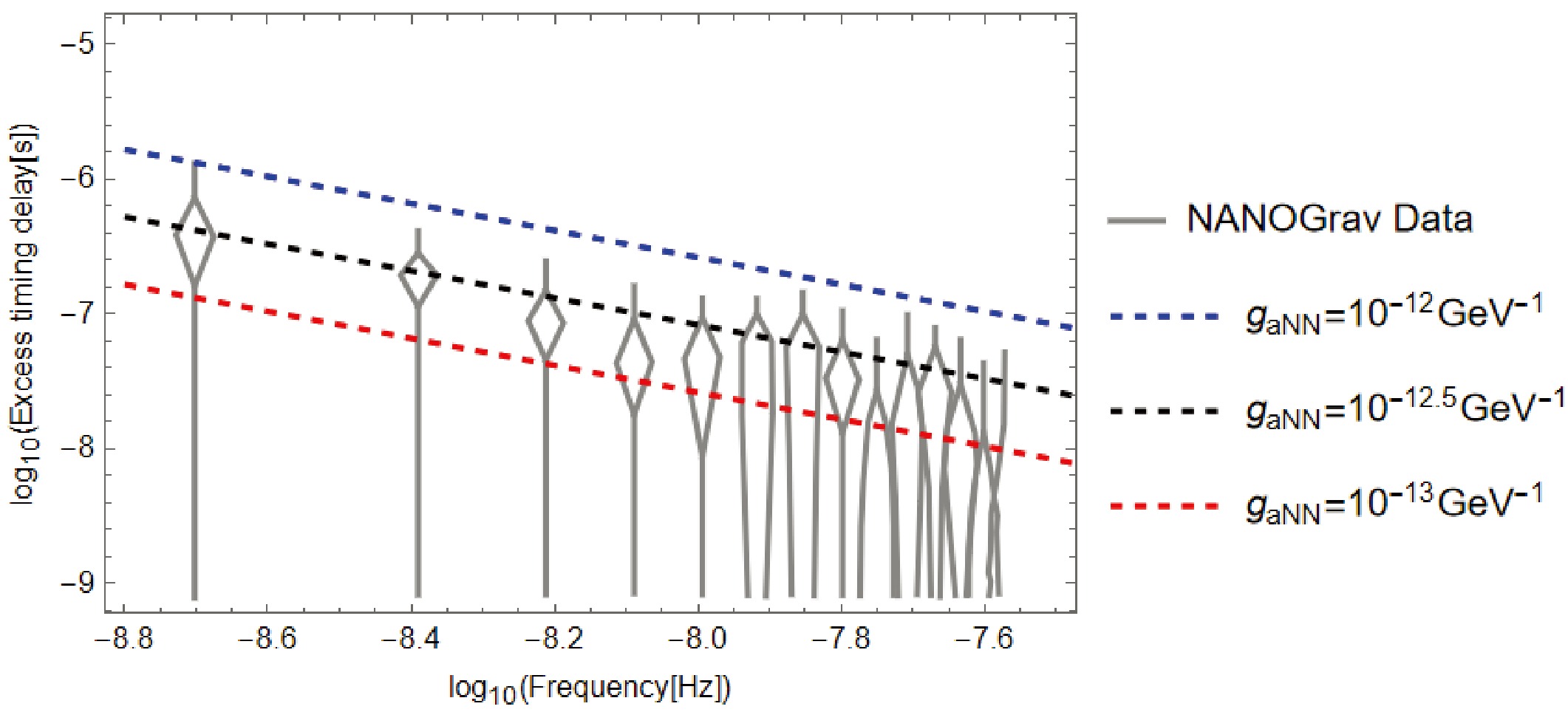

Figure 1.  (color online) Upper limits on the timing residual of pulsar generated by the oscillating dark matter, as a function of frequency/axion's mass. The gray line is the recently released NanoGrav data[20]. The blue, black, and red lines are the upper limits for the coupling constant $ g_{aNN} $ equals $ 10^{-12}\mathrm{GeV}^{-1}, 10^{-12.5}\mathrm{GeV^{-1}, 10^{-13}\mathrm{GeV}^{-1}} $ respectively.

The cross-correlation Hellings-Downs curve between the noise-independent data is essential to detect the gravitational wave background[103, 104]. The cross-correlation between the timing residuals of the pulsar a and b can be calculated through $ \langle z_a\left(t\right)z_b\left(t\right)\rangle $, where $ \langle \cdots \rangle $ represents a time average or an ensemble average. Having the explicit form of the redshift $ z\left(t\right) $ in hand, we can then calculate,

To simplify the calculation below, we then choose another frame that contains the pulsar location unit vector which points from the Earth towards the pulsar as the initial direction:

Without losing generality we set the initial direction of the magnetic axis of the pulsars a and b as:

We also set the orientation of the axion's velocity and the rotational axes of pulsars a and b:

According to Eq.(15), we can easily calculate S of pulsar a and b:

The pulsars we observe are distributed all over the sky; we can assume that their relative angles to the direction of the axion's velocity are random. This means that the average of the cross-correlation signals among many pulsars effectively takes an average over the direction of the axion's velocity. The rotational axis can also change its direction as a result of the motion of the galaxy, so we also take an average over the rotational axis and perform the integral over $ \hat{v}, \hat{\Omega}_{0a}, \hat{\Omega}_{0b} $:

This curve is similar to the vector type modes in massive gravity types of studies [74, 103, 105−107] as expected, due to the one-dimensional directional nature of this modulation. We plot this axion-nucleon curve in Fig. 2. Notice here we did not impose NANOGrav data constraints on the dipole term, and the curve presented was derived purely from theoretical considerations.

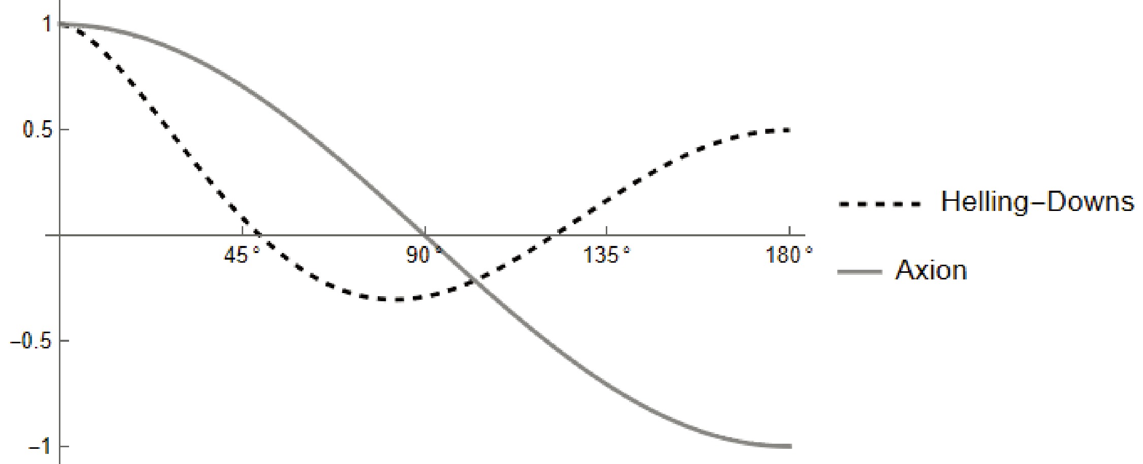
Figure 2.  The angle of separation dependence of the two-point correlation function, normalized to $ 1 $ when $ \theta=0 $. The dashed curve corresponds to the angular correlation of the timing residuals induced by the gravitational wave background(Hellings-Downs curve), and the solid line represents the correlation of the axion's effect acting on the pulsars.

We consider a new detection possibility of employing neutron stars as axion wind detectors. Current PTA network observations can provide interesting sensitivity to the axion-nucleon couplings. This classical macroscopic detection mechanism is complementary to the axion microscopic production and capture mechanism [94, 108−113] to set the limits on the related coupling. Due to the complexity of the neutron star structure models, we expect noise from several different sources to affect the neutron star's motion. Nevertheless, a close analysis of neutron star behavior might provide further insight into this type of coupling. Those analyses will represent a specialized component of our data processing pipeline, specifically addressing noise signal properties. We will investigate those in future work to enhance the robustness of our approach.

We thank Fei Gao for the discussion on the neutron stars.