Unveiling the electromagnetic structure and intrinsic dynamics of spin-$ \bf{3/2}$ hidden-charm pentaquarks: A comprehensive QCD analysis

The study of multiquark states, including tetraquarks, hybrids, glueballs, and pentaquarks, along with the conventional meson-baryon states, has emerged as a pivotal subject in the field of hadron physics after their introduction within the framework of the quark model. Given that Quantum Chromodynamics (QCD) does not inherently preclude their existence, these multiquark states have garnered the interest of the hadron physics community from its inception and have been the subject of comprehensive investigation over an extended period. Following an extended period of anticipation, the much-speculated existence of these states was finally confirmed in 2003 with the announcement of the discovery of the X(3872) particle by the Belle Collaboration [1]. This discovery was identified as a candidate tetraquark state, signifying a substantial advancement in the domain of particle physics. Subsequently, the observation of a large number of promising candidates for multi-quark states by different experimental collaborations contributed to an increase in our expectations and understanding in the field of particle physics.

Following the discovery in 2003, in 2015, the LHCb Collaboration observed a new member of the exotic states, the pentaquark state, which consists of five valence quarks. A detailed analysis of the $ J /\psi + p $ decay channel revealed two pentaquark candidates, designated as $ P_c(4380) $ and $ P_c(4450) $ [2]. In 2019, a more extensive analysis was conducted using a larger data sample, providing further information. It was reported that the previously identified $ P_c(4450) $ pentaquark candidate splits into $ P_c(4440) $ and $ P_c(4457) $ states, revealing an additional peak: the $ P_c(4312) $ state [3]. It is noteworthy that the final status of the $ P_c(4380) $ pentaquark, as reported in the 2015 analysis, remains unresolved, neither confirmed nor ruled out in the updated 2019 analysis. In 2020, the LHCb Collaboration unveiled an additional pentaquark state, designated as $ P_{cs} (4459) $, within the invariant mass spectrum of $ J /\psi\Lambda $ [4]. In 2022, the LHCb Collaboration made a notable observation: a novel structure, $ P_{cs} (4338) $, was identified within the $ J /\psi\Lambda $ mass distribution in the $ B^- \to J /\psi\Lambda^- p $ decays [5]. In 2024, the Belle Collaboration used $ \Upsilon(1S,2S) $ events to search for the pentaquark state in the $ pJ/\psi $ final state. No significant $ P_{c} (4312) $, $ P_{c} (4440) $, or $ P_{c} (4457) $ signal was observed in the $ pJ/\psi $ final state in $ \Upsilon(1S,2S) $ inclusive decays [6]. Very recently, the Belle Collaboration found evidence for the $ P_{cs}(4459) $ state with a significance of 3.3 standard deviations, including statistical and systematic uncertainties [7]. A compendium of data on the mass, width, minimal valence quark content, and observed channel for these states is provided in Table 1. Along with the aforementioned hidden-charm pentaquark states, the search for doubly and triply strange hidden-charm pentaquarks is currently underway, with the CMS Collaboration recently observing the decay $ \Lambda_b^0\to J/\psi\Xi^-K^+ $ [8]. Nevertheless, insufficient yield and inadequate resolution prevented the observation of a clear spectrum in the $ J/\psi\Xi^- $ invariant mass. These findings are relevant for illuminating the strong interaction processes that underlie the hadronic decays of beauty baryons and the underlying potential mechanism for the production of multiquark states.

State	Mass/MeV	Width/MeV	Quark content	Observed decays
$ P_c(4312)^+ $ [3]	$ 4311.9\pm0.7^{\; +6.8}_{\; -0.6} $	$ 9.8\pm2.7^{\; +3.7}_{\; -4.5} $	$ uudc\bar{c} $	$ \Lambda_b^0 \to J/\psi pK^- $
$ P_c(4440)^+ $ [3]	$ 4440.3\pm1.3^{\; +4.1}_{\; -4.7} $	$ 20.6\pm4.9^{\; +8.7}_{\; -10.1} $	$ uudc\bar{c} $	$ \Lambda_b^0 \to J/\psi pK^- $
$ P_c(4457)^+ $ [3]	$ 4457.3\pm0.6^{\; +4.1}_{\; -1.7} $	$ 6.4\pm2.0^{\; +5.7}_{\; -1.9} $	$ uudc\bar{c} $	$ \Lambda_b^0 \to J/\psi pK^- $
$ P_{cs}(4459)^0 $ [4]	$ 4458.8\pm2.9^{\; +4.7}_{\; -1.1} $	$ 17.3\pm6.5^{\; +8.0}_{\; -5.7} $	$ udsc\bar{c} $	$ \Xi_b^- \to J/\psi \Lambda K^- $
$ P_{cs}(4338)^0 $ [5]	$ 4338.2 \pm 0.7 \pm 0.4 $	$ 7.0 \pm 1.2 \pm 1.3 $	$ udsc\bar{c} $	$ B^-\to J/\psi \Lambda \bar{p} $
$ P_{cs}(4459)^0 $ [7]	$ 4471.7 \pm 4.8 \pm 0.6 $	$ 21.9 \pm 13.1 \pm 2.7 $	$ udsc\bar{c} $	$ \Upsilon (1S, 2S)\to J/\psi \Lambda $

Table 1.  Reported hidden-charm pentaquark states by the LHCb [2−5] and Belle [7] Collaborations.

Several interpretations have been posited for these pentaquark states, including the hypothesis of tightly-bound pentaquark states, loosely-bound meson-baryon molecular states, and the product of re-scattering effects, among others. For a more detailed discussion, see Refs. [9−26]. Despite the significant body of research published since the initial observation of these states, our understanding of their precise nature, internal structure, and crucial parameters such as spin-parity quantum numbers remains incomplete. Significant effort is still required to address the aforementioned gaps. In addition to the discovered pentaquark states $ P_c(4312) $, $ P_c(4440) $, $ P_c(4457) $, $ P_{cs}(4338) $, and $ P_{cs}(4459) $, searching for other possible pentaquarks containing one or two strange quarks or those without strangeness and determining their properties are also important and interesting topics of study. One of the key tools for probing the internal structure of hadrons is the study of their electromagnetic properties, such as magnetic dipole moments, electric quadrupole moments, and higher-order multipole moments. These properties are sensitive to the spatial distribution of quarks and their spin orientations within the hadron. For hidden-charm pentaquarks, the electromagnetic multipole moments can provide critical insights into their quark-gluon composition, spin-parity assignments, and geometric shape. To this end, the present study investigates the magnetic dipole, electric quadrupole, and magnetic octupole moments of the $ [u u][d c] \bar c $, $ [dd][u c] \bar c $, $ [u u][s c] \bar c $, $ [dd] [s c] \bar c $, $ [s s][u c] \bar c $, and $ [s s][d c] \bar c $ states in the context of the QCD light-cone sum rules [27−29]. In the course of examining these properties, two distinct diquark-diquark-antiquark forms of the interpolating currents are employed since these pentaquark candidates have the quantum numbers $ {{J}^{P} = {3}/{2}^-} $. By calculating the magnetic dipole, electric quadrupole, and magnetic octupole moments, we aim to shed light on the internal structure of these exotic states and make predictions that can be tested in future experiments. Our results not only contribute to the ongoing effort to understand the nature of pentaquarks but also offer valuable insights into the dynamics of multiquark systems in QCD. Despite their importance, the electromagnetic properties of hidden-charm pentaquarks have not been extensively studied, either theoretically or experimentally. The extant literature offers limited coverage of the electromagnetic multipole moments of hidden-charm/bottom pentaquarks [30−52].

This paper is organized as follows. Sec. II outlines the QCD light-cone sum rules utilized to calculate the magnetic dipole, electric quadrupole, and magnetic octupole moments of the states considered in this study. In Sec. III, we present the numerical analysis of the results derived from the QCD light-cone sum rules. The final section offers a summary and conclusion based on the findings.

To facilitate the analysis of the electromagnetic multipole moments of the $ P_{c(s)} $ states, the correlation function that must be used in the analysis should be determined. The following formula was determined to be the appropriate correlation function:

where $ J_{\mu}^i(x) $ represents the interpolating current of the $ P_{c(s)} $ states, γ is the external electromagnetic field, and q is the momentum of the photon. To study the electromagnetic multipole moments of $ P_{c(s)} $ pentaquarks, the $ J_{\mu}^i(x) $ interpolating currents prove to be significant and can be considered pivotal parameters. Considering the quark content and spin-parity quantum numbers of the pentaquarks in question, the interpolating currents that are likely to couple to the pentaquarks with spin-parity quantum numbers $ {{J}^{P} = {3}/{2}^-} $ are expressed as follows [53]:

where $ {\cal{A}} = \varepsilon_{abc}\varepsilon_{ade} \varepsilon_{bfg} $, with a, b, c, d, e, f, and g being the color indices, and C is the charge conjugation operator. The quark content of the $ P_{c(s)} $ states is listed in Table 2. We should note that the interpolating currents considered here may also couple to positive-parity pentaquark states. According to Refs. [53−56], pentaquarks with positive parity have higher masses than those with negative parity states. This mass difference is particularly relevant in magnetic moment calculations, where contributions from higher-mass states are typically neglected due to their suppressed effects. Since the pentaquarks studied in this work are low-mass states, it is reasonable to disregard the already small contribution of the spin-$ {3}/{2}^+ $ pentaquark states in the magnetic moment analysis. Therefore, the interpolating current used predominantly couples to the spin-$ {3}/{2}^- $ pentaquarks, and the resulting magnetic moment values correspond primarily to these states.

States	$ [u u][d c] \bar c $	$ [dd][u c] \bar c $	$ [u u][s c] \bar c $	$ [dd ][s c] \bar c $	$ [s s][u c] \bar c $	$ [s s][d c] \bar c $
$ q_1 $	u	d	u	d	s	s
$ q_2 $	d	u	s	s	u	d

Table 2.  The quark content of the $ P_{c(s)} $ states.

The essential parameters necessary to initiate the analysis are derived within the framework of the pertinent methodology. As a preliminary step, we derive some of the analytical expressions for the electromagnetic multipole moments using the hadronic description of the correlation function.

In the context of the hadron description, a complete set of intermediate hadronic states is inserted into the correlation function, each state being assigned the same quantum numbers as the interpolating currents. The ground-state contributions are then isolated. Consequently, we get

where $ p_1 = p+q $, $ p_2 = p $. An examination of Eq. (4) shows that various matrix elements with different structures are required in the subsequent analysis. These matrix elements are outlined below [57−60]:

where $ \lambda_{P_{c(s)}} $ is pole residue (or coupling) of the $ P_{c(s)} $ states, $ u_{\mu}(p_2,s) $ and $ \bar u_{\nu}(p_1,s) $ are the spinors of the $ P_{c(s)} $ states, ε is the photon's polarization vector, and $ F_i (q^2) $ are transition form factors. Using Eqs. (4) to (7) and making the requisite simplifications, the expressions for the magnetic moment of the $ P_{c(s)} $ states in conjunction with hadronic parameters are as follows:

To derive the aforementioned equation, a sum over the spins of the $P_{c(s)}$ state must be performed as follows:

The Lorentz invariant form factors $ F_{1}(q^2) $, $ F_{2}(q^2) $, $ F_{3}(q^2) $, and $ F_{4}(q^2) $ are related to the magnetic dipole, $ G_{M}(q^2) $, electric quadrupole, $ G_{Q}(q^2) $, and magnetic octupole, $ G_{O}(q^2) $, form factors as [57−60]

where $ \tau = -\dfrac{q^2}{4m^2_{P_{c(s)}}} $is a kinematic factor. These expressions enable the extraction of the electromagnetic form factors for these pentaquark states. At zero momentum transfer, since we deal with a real photon ($ q^2 = 0 $), these form factors are proportional to the usual static quantities of the magnetic dipole ($ \mu_{P_{c(s)}} $), the electric quadrupole ($ Q_{P_{c(s)}} $), and the magnetic octupole ($ O_{P_{c(s)}} $) moments of the $ P_{c(s)} $ states:

where

Along with the derivation of the above expressions, the hadronic description of the correlation function corresponding to the magnetic dipole, electric quadrupole, and magnetic octupole moments of the pentaquark states is obtained.

In the following, we provide a concise overview of the operator product expansion for the correlation function in perturbative QCD. To that end, the quark fields in the correlation function are contracted using the Wick theorem. Using the $ J_\mu^1 $ current as an example, this would result in the following:

where the light and charm quark propagators, denoted by $ S_q(x) $ and $ S_c(x) $, respectively, can be expressed as follows [61, 62]

with

where $ G^{\mu\nu} $ is the gluon field strength tensor and $ K_n $ are modified Bessel functions of the second kind.

The QCD description has two classes of contributions according to the way the photon interacts with the quark lines. First, the photon interacts perturbatively with the quark line through the standard QED interaction. In this set of interactions, it is possible to replace one of the free quark propagators in Eq. (13) with a propagator that incorporates an electromagnetic interaction. This replacement can be achieved by employing the following method:

The second category of interactions encompasses the non-perturbative interaction of photons with quarks, as depicted by the photon light cone distribution amplitude. One of the five propagators in Eq. (13) is replaced by

where $ \Gamma_i=\mathrm{1},\gamma_5,\gamma_{\mu},\mathrm{i}\gamma_5\gamma_{\mu},\sigma_{\mu\nu}/2 $. Upon substituting the replacement stipulated in Eq.(19), expressions such as $ \langle \gamma(q)\left| \bar{q}(x) \Gamma_i G_{\mu\nu}q(0) \right| 0\rangle $ and $ \langle \gamma(q)\left| \bar{q}(x) \Gamma_i q(0) \right| 0\rangle $ are derived. These expressions are obtained in the form of photon dispersion amplitudes within the framework of the requisite analysis (for details see Ref. [63]). As these subjects are thoroughly delineated and have been standardized, we avoid further elaboration in this section. For a more comprehensive description of these subjects, please refer to Refs. [64, 65]. Eqs. (18) and (19) have been utilized to encompass both perturbative and non-perturbative contributions within the conducted analysis under the prescribed scheme.

The findings from evaluations on both descriptions of the correlation function are compared using dispersion relations that consider the coefficients of the same Lorentz structures. In the final step, double Borel transformations are applied to variables $ -p^2 $ and $ -(p+q)^2 $. This process eliminates contributions from the continuum and higher states, thereby enhancing contributions from ground states. To illustrate this, consider the case of the magnetic dipole moment. The results obtained using the double dispersion relations are as follows [66, 67]:

where $ m_1(m_2) $, $ s_1(s_2) $ and $ M_1^2(M_2^2) $ are the mass, continuum threshold, and Borel parameter for the initial (final) $ P_{c(s)} $ tetraquarks, respectively, and $ \cdots $denote the contribution from higher states and the continuum. $ \rho(s_1, s_2) $ denotes the hadronic spectral density, which is obtained through double Borel transformations applied to the correlation function.

To calculate the magnetic dipole moment within the QCD light-cone sum rules, it is necessary to extract the contributions from higher states and the continuum. This is achieved by utilizing the quark-hadron duality ansatz as follows:

where $ \mathbb D $ is a domain in the $ (s_1,s_2) $ plane. Generally, the domain $ \mathbb D $ is a rectangular region defined by $ s_1<s_{10} $ and $ s_2<s_{20} $ for some constants $ s_{10} $ and $ s_{20} $ or a triangular region. For brevity, we perform the continuum subtraction by selecting $ \mathbb D $ as the region specified by $ s \equiv s_1 u_0 + s_2 \bar u_0 < s_0 $, where $ u_0\equiv \dfrac{M_2^2}{M_1^2+M_2^2} $ and $ \bar u_0 = 1 - u_0 $. Defining a second variable $ u = \dfrac{s_1 u_0}{s} $, the integral in the $ (s_1,s_2) $ plane can be defined as:

where

For the considered problem, the masses of the initial and final states are the same; hence, we can set $ M_1^2 = M_2^2 = 2M^2 $, which produces $ u_0 = {1}/{2} $. Based on the aforementioned procedure, the continuum subtraction performed by setting the upper limit to $ s_0 $ is equivalent (in the original double spectral density) to subtracting everything outside the triangular region $ s = s_1 u_0 + s_2 \bar u_0 \equiv s_0 $. Following this scheme, the QCD light-cone sum rules for the $ F_1 $, $ F_2 $, $ F_3 $, and $ F_4 $ form factors can be determined by equating the coefficients of the $ g_{\mu\nu}{\not {p }} {\not {\varepsilon }}{\not {q }} $, $ g_{\mu\nu}{\not {\varepsilon }}{\not {q }} $, $ q_{\mu}q_{\nu}{\not {\varepsilon }}{\not {q }} $, and $ (\varepsilon.p)q_{\mu}q_{\nu}{\not {p }} {\not {q }} $ structures. The obtained sum rules for the electromagnetic multipole moments of the$ P_{c(s)} $ states are presented as follows:

Since the forms of the $ \rho_i (\rm{M^2},\rm{s_0}) $ functions are similar, for illustrative purposes, we only present the explicit form of the $ \rho_1 (\rm{M^2},\rm{s_0}) $, $ \rho_2 (\rm{M^2},\rm{s_0}) $, and $ \rho_3 (\rm{M^2},\rm{s_0}) $ functions in the Appendix.

The following section is concerned with the results of a numerical analysis of the QCD light-cone sum rules. This analysis is conducted to predict the electromagnetic multipole moments of the $ P_{c(s)} $ states. To perform a numerical analysis of the QCD light-cone sum rule, it is first necessary to ascertain the numerical values of several parameters. The following numerical values are assigned to the relevant parameters: $ m_s = 93.4^{+8.6}_{-3.4}\,\text{MeV} $, $ m_c = 1.27 \pm 0.02\,\text{GeV} $ [68], $ m_{[uu][dc]\bar c} = $ $ m_{[dd][uc]\bar c} = $ $ 4.39 \pm 0.14 $ GeV [53], $ m_{[uu][sc]\bar c} = $ $ m_{[dd][sc]\bar c} = $ $ 4.51 \pm 0.12 $ GeV [53], $ m_{[ss][uc]\bar c} = $ $ m_{[ss][dc]\bar c} = $ $ 4.60 \pm 0.11 $ GeV [53], $ \langle \bar uu\rangle = \langle \bar dd\rangle = (-0.24 \pm 0.01)^3\,\text{GeV}^3 $, $ \langle \bar ss\rangle = (0.8 \pm 0.1)\, \langle \bar uu\rangle $ $ \,\text{GeV}^3 $ [69], $ m_0^{2} = 0.8 \pm 0.1 \,\text{GeV}^2 $ [69], and $ \langle g_s^2G^2\rangle = 0.48 \pm 0.14\; \text{GeV}^4 $ [70]. Furthermore, the residues of the $ P_{c(s)} $ states are required, as adopted from Ref. [53]. In numerical calculations, the parameters $ m_u $, $ m_d $, and $ m_s^2 $ are set to zero because their contributions are substantially small. However, it is important to note that terms proportional to $ m_s $ are considered. For further calculations, the photon DAs and their explicit form, as well as the required numerical quantities, must be used, as described in Ref. [63].

In light of the preceding numerical input variables, two supplementary parameters must be incorporated into the execution of this numerical analysis. The first of these is the continuum threshold parameter, designated as $ {{\rm{s}}_0} $. The second is the Borel mass parameter, denoted by $ {{\rm{M}}^2} $. In an ideal scenario, the numerical analysis should be performed independently of the parameters mentioned above. However, this approach is neither pragmatic nor realistic. Establishing a region of analysis is imperative to ensure that the effect of parameter variation on the numerical results is negligible. The parameter $ {{\rm{s}}_0} $ is not arbitrary; rather, it establishes a scale. Subsequent to this scale, continuum and higher states begin to influence the correlation function. Although various methods for determining the working region of this parameter have been proposed, it has been observed to be within the range $ (m_{P_{c(s)}} +0.5)^2 $ GeV² $ \leq $ $ {{\rm{s}}_0} $ $ \leq $ $ (m_{P_{c(s)}} +0.8)^2 $GeV². Therefore, an approach that assumes that the parameter is within this working interval is preferred. The working region for $ {{\rm{M}}^2} $, that is, the range in which the variation in our numerical predictions of the variable is relatively small, is constrained by the applied approaches. The aforementioned constraints are referred to as the pole contribution (PC) and convergence of OPE (CVG). Following the prevailing methodology, the CVG must be sufficiently small for the OPE to converge. Conversely, the PC is assumed to be adequately large to improve the efficiency of the single-pole scheme. The following formulas have been used to quantify them:

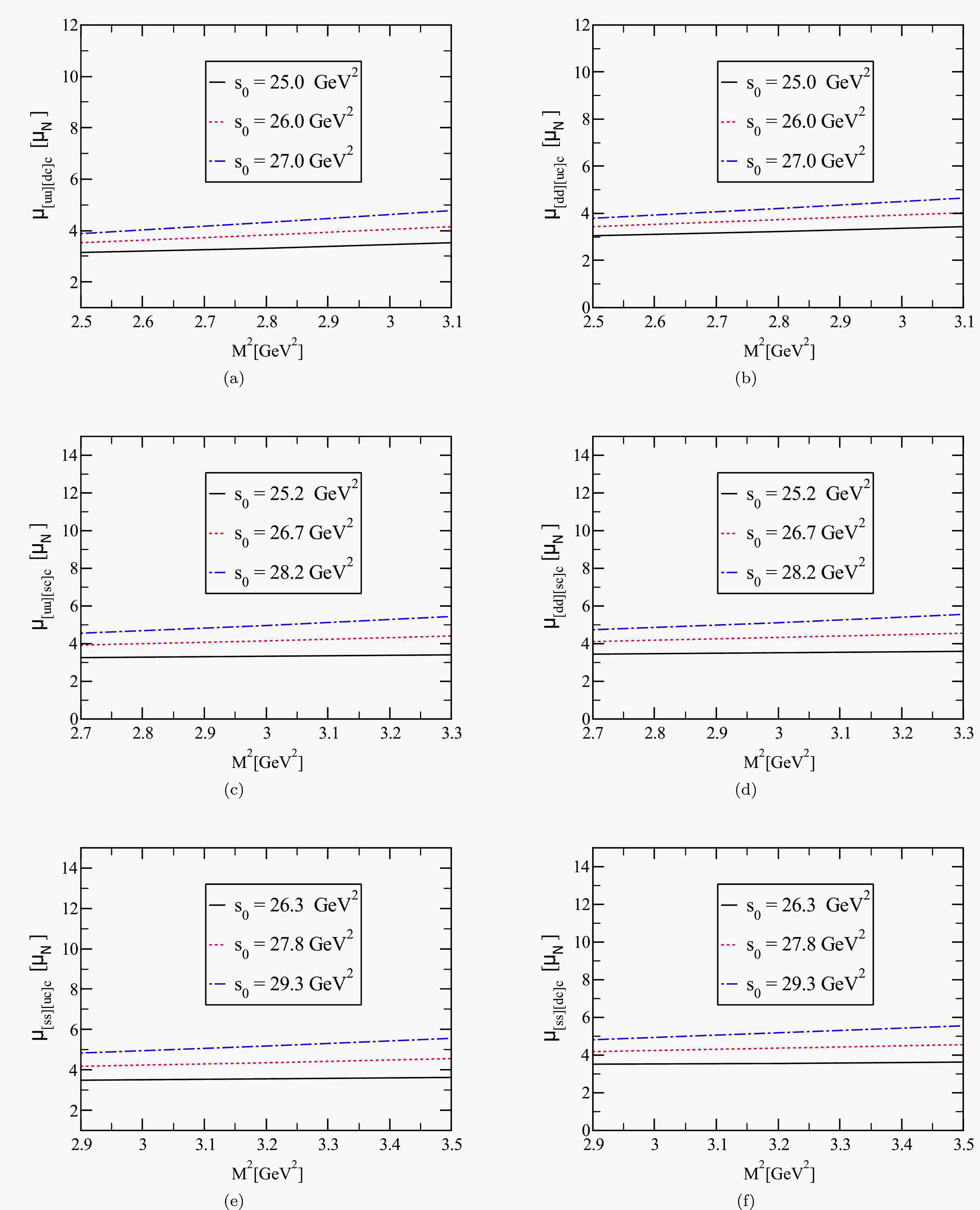
where $ \rho_i^{\rm{DimN}} (\rm{M^2},\rm{s_0}) $ represents the highest dimensional terms in $ \rho_i (\rm{M^2},\rm{s_0}) $. As demonstrated in the analytical expressions in the appendix, our analysis incorporates combinations of condensates with varying compositions, such as $ \langle g_s^2G^2\rangle \langle \bar q q\rangle^2 $, $ m_0^2 $ $ \langle g_s^2G^2\rangle \langle \bar q q\rangle $, $ \langle g_s^2G^2\rangle \langle \bar q q\rangle $, $ \langle \bar q q\rangle^2 $, $ \langle g_s^2G^2\rangle $, and $ \langle \bar q q\rangle $. In our analysis, the highest dimensional terms are dimension 8 ($ m_0^2 $ $ \langle \bar q q\rangle^2 $), 9 ($ m_0^2 $ $ \langle g_s^2G^2\rangle \langle \bar q q\rangle $), and 10 ($ \langle g_s^2G^2\rangle \langle \bar q q\rangle^2 $). Consequently, the CVG analysis has been performed by considering the DimN expression in the form of $ \rm{Dim(8+9+10)} $. From our analysis, considering the results in Table 3, the working regions of parameters $ {{\rm{s}}_0} $ and $ {{\rm{M}}^2} $ meet the constraints of the method. To ensure that the study regions are consistent, the magnetic dipole moments at different values of $ {{\rm{s}}_0} $ are plotted against $ {{\rm{M}}^2} $ in Figs. 1 and 2. As demonstrated in these figures, the variation of the magnetic dipole moment resulting from these parameters is within an acceptable limit. It is also worth noting that the results may be affected by uncertainty due to the presence of residual dependencies.

Current	State	$ \mathrm{s_0} $/GeV2	$ \mathrm{M^2} $/GeV2	CVG(%)	PC(%)	Pert(%)	NPert(%)
$ J_\mu^1 $	$ [uu] [dc] \bar c $	$ [25.0, 27.0] $	$ [2.5, 3.1] $	$ \ll 1 $	[56.45, 35.38]	$ (88-93) $	$ (7-12) $
	$ [dd] [uc] \bar c $	$ [25.0, 27.0] $	$ [2.5, 3.1] $	$ \ll 1 $	[56.36, 35.27]	$ (88-93) $	$ (7-12) $
	$ [uu] [sc] \bar c $	$ [25.2, 28.2] $	$ [2.7, 3.3] $	$ \ll 1 $	[56.15, 34.60]	$ (89-94) $	$ (6-11) $
	$ [dd] [sc] \bar c $	$ [25.2, 28.2] $	$ [2.7, 3.3] $	$ \ll 1 $	[56.12, 35.78]	$ (87-92) $	$ (8-13) $
	$ [ss] [uc] \bar c $	$ [26.3, 29.3] $	$ [2.9, 3.5] $	$ \ll 1 $	[55.08, 34.90]	$ (89-94) $	$ (6-11) $
	$ [ss] [dc] \bar c $	$ [26.3, 29.3] $	$ [2.9, 3.5] $	$ \ll 1 $	[56.30, 36.05]	$ (87-92) $	$ (8-13) $
$ J_\mu^2 $	$ [uu] [dc] \bar c $	$ [25.0, 27.0] $	$ [2.5, 3.1] $	$< 1.5 $	[57.45, 35.38]	$ (81-86) $	$ (14-19) $
	$ [dd] [uc] \bar c $	$ [25.0, 27.0] $	$ [2.5, 3.1] $	$< 1.5 $	[57.36, 35.27]	$ (81-86) $	$ (14-19) $
	$ [uu] [sc] \bar c $	$ [25.2, 28.2] $	$ [2.7, 3.3] $	$< 1.5 $	[57.23, 35.47]	$ (80-85) $	$ (15-20) $
	$ [dd] [sc] \bar c $	$ [25.2, 28.2] $	$ [2.7, 3.3] $	$< 1.5 $	[54.17, 35.24]	$ (75-82) $	$ (18-25) $
	$ [ss] [uc] \bar c $	$ [26.3, 29.3] $	$ [2.9, 3.5] $	$< 1.5 $	[53.97, 34.14]	$ (80-85) $	$ (15-20) $
	$ [ss] [dc] \bar c $	$ [26.3, 29.3] $	$ [2.9, 3.5] $	$< 1.5 $	[53.64, 33.17]	$ (75-82) $	$ (18-25) $

Table 3.  Working regions of $ \rm{s_0} $ and $ \rm{M^2} $ together with the CVG and PC for the magnetic moments of the $ P_{c(s)} $ states, where "Pert" and "NPert" represent contributions from the perturbative and non-perturbative terms, respectively.

Figure 1.  (color online) Magnetic dipole moments of the $P_{c(s)} $ states versus $\mathrm{M^2} $ for the $J_\mu^1 $ current.

Figure 2.  (color online) Magnetic dipole moments of the $P_{c(s)} $ states versus $\mathrm{M^2} $ for the $J_\mu^2 $ current.

All the necessary variables for the numerical evaluation are determined. The entire numerical predictions, together with all the inherent uncertainties concerning the input quantities, are listed in Table 4. The following conclusions can be made from the results:

Current	Pentaquarks	$ \mu\,(\mu_N) $	$ {\cal{Q}} $/($ 10^{-2} $ fm2)	$ {\cal{O}} $/($ 10^{-3} $ fm3)
$ J_\mu^1 $	$ [uu] [dc] \bar c $	$ 3.95 \pm 0.82 $	$ 0.31 \pm 0.02 $	$ - 0.56 \pm 0.07 $
	$ [dd] [uc] \bar c $	$ 3.86 \pm 0.80 $	$ 1.79 \pm 0.23 $	$ - 0.81 \pm 0.07 $
	$ [uu] [sc] \bar c $	$ 4.33 \pm 1.09 $	$ 0.32 \pm 0.02 $	$ - 0.58 \pm 0.08 $
	$ [dd] [sc] \bar c $	$ 4.50 \pm 1.04 $	$ 3.48 \pm 0.60 $	$ -1.09 \pm 0.08 $
	$ [ss] [uc] \bar c $	$ 4.53 \pm 1.03 $	$ 1.83 \pm 0.28 $	$ -0.80 \pm 0.08 $
	$ [ss] [dc] \bar c $	$ 4.48 \pm 0.98 $	$ 3.42 \pm 0.56 $	$ -1.04 \pm 0.08 $
$ J_\mu^2 $	$ [uu] [dc] \bar c $	$ 3.17 \pm 0.82 $	$ -1.43 \pm 0.26 $	$ - 0.20 \pm 0.04 $
	$ [dd] [uc] \bar c $	$ 3.09 \pm 0.61 $	$ \; \; 1.51 \pm 0.19 $	$ - 0.62 \pm 0.05 $
	$ [uu] [sc] \bar c $	$ 3.43 \pm 0.83 $	$ -1.53 \pm 0.33 $	$ - 0.21 \pm 0.05 $
	$ [dd] [sc] \bar c $	$ 2.19 \pm 0.59 $	$ \; \; 4.85 \pm 0.88 $	$ -1.12 \pm 0.07 $
	$ [ss] [uc] \bar c $	$ 2.81 \pm 0.67 $	$ \; \; 1.57 \pm 0.25 $	$ -0.63 \pm 0.06 $
	$ [ss] [dc] \bar c $	$ 1.84 \pm 0.49 $	$ \; \; 4.80 \pm 0.82 $	$ -1.06 \pm 0.06 $

Table 4.  Predictions of the electromagnetic multipole moments of the $ P_{c(s)} $ states.

● In the QCD light-cone sum rules framework, the primary contributions to the electromagnetic multipole moments of the $ P_{c(s)} $ states originate from the perturbative component of the spectral density. This component can be schematically expressed as $ ( A \, e_c \pm B \, (2 e_{q_1}+e_{q_2})) $. For the magnetic dipole moment, the contribution from the $ B \, (2 e_{q_1}+e_{q_2}) $ term is found to be negligible. However, for the electric quadrupole and magnetic octupole moments, this term plays a more significant role, and in some cases, it determines the sign of the electric quadrupole moment in certain $ P_{c(s)} $ states.

● A more thorough investigation of the magnetic dipole moment requires the examination of the contributions of light quarks and the charm quark. The findings of this comprehensive analysis are presented in Table 5 , where the central values of all input parameters are used. The contributions of both light quarks and the charm quark differ significantly depending on the choice of interpolating current. For the $ J_\mu^1 $ interpolating current, the contributions of light quarks to the magnetic dipole moment are quite small. In contrast, for the $ J_\mu^2 $ interpolating current, these contributions become larger than in the $ J_\mu^1 $ interpolating current. The analysis of quark contributions to the magnetic dipole moments reveals that the charm quark dominates the magnetic properties of pentaquarks. The light quarks (up, down, and strange) contribute less significantly to the magnetic dipole moments. However, their contributions vary depending on the diquark configuration. This variation suggests that the light quark dynamics are sensitive to the quark arrangement within the pentaquark.

Current	Pentaquarks	$ \mu_{q} $	$ \mu_{c} $	$ \mu_{\rm total} $
$ J_\mu^1 $	$ [uu] [dc] \bar c $	$ -0.30 $	$ 4.25 $	$ 3.95 $
	$ [dd] [uc] \bar c $	$ -0.31 $	$ 4.17 $	$ 3.86 $
	$ [uu] [sc] \bar c $	$ -0.27 $	$ 4.60 $	$ 4.33 $
	$ [dd] [sc] \bar c $	$ -0.11 $	$ 4.61 $	$ 4.50 $
	$ [ss] [uc] \bar c $	$ -0.17 $	$ 4.70 $	$ 4.53 $
	$ [ss] [dc] \bar c $	$ -0.21 $	$ 4.69 $	$ 4.48 $
$ J_\mu^2 $	$ [uu] [dc] \bar c $	$ \; \; 0.21 $	$ 2.96 $	$ 3.17 $
	$ [dd] [uc] \bar c $	$ \; \; 0.14 $	$ 2.95 $	$ 3.09 $
	$ [uu] [sc] \bar c $	$ \; \; 0.26 $	$ 3.17 $	$ 3.43 $
	$ [dd] [sc] \bar c $	$ -0.98 $	$ 3.17 $	$ 2.19 $
	$ [ss] [uc] \bar c $	$ -0.41 $	$ 3.22 $	$ 2.81 $
	$ [ss] [dc] \bar c $	$ -1.38 $	$ 3.22 $	$ 1.84 $

Table 5.  Contributions of light and heavy quarks to the magnetic dipole moment of the $ P_{c(s)} $ states ($ \mu_N $).

● The contributions of charm- and light quarks to the magnetic dipole moment are observed to exhibit an inverse relationship, except for the $ [u u][d c] \bar c $, $ [dd][u c] \bar c $, and $ [uu][sc] \bar c $ states, which are obtained in the case of $ J_\mu^2 $. The signs of the magnetic dipole moments demonstrate the interaction of the spin degrees of freedom of the quarks. The opposite signs of the magnetic dipole moments for charm and light quarks suggest that their spins are anti-aligned within the pentaquark.

● The electric quadrupole and magnetic octupole moments of the related pentaquarks are also calculated. The obtained results are given in Table 4. It may be posited that the values of the electric quadrupole and magnetic octupole moments are substantially smaller than those of the magnetic dipole moments. This finding indicates the presence of non-zero values for the electric quadrupole and magnetic octupole moments of the observed pentaquarks, suggesting a non-spherical charge distribution. The sign of the electric quadrupole moment reveals the overall shape of the charge distribution in the baryon states: a positive quadrupole moment indicates a prolate deformation — charge is stretched along the quantization axis. A negative quadrupole moment indicates an oblate deformation — charge is concentrated in the transverse plane. The magnetic octupole moment gives information about the spatial distribution of the magnetic current inside the baryon: a positive octupole moment suggests that magnetic currents are aligned or concentrated along a specific axis. A negative octupole moment indicates an opposite orientation of the magnetic current distribution. It can be posited that the signs of the higher multipole moments can offer insights into the deformation of the corresponding hadron and its direction. If the signs of the higher multipole moments are the same, the geometric deformation and the charge distribution are in the same direction. Conversely, if the signs are different, the spatial deformation and charge distribution are in opposite orientations. For a negative prediction, the hadron is oblate, and for a positive prediction, it is prolate. The electric quadrupole moments is predicted to be positive except in the $ [u u][d c] \bar c $ and $ [uu][sc]\bar c $ states, which are obtained for $ J_\mu^2 $ and correspond to the prolate charge distribution. In contrast, the sign of the magnetic octupole moments is negative. This finding suggests that the charge distribution and geometrical shape of these states are opposite. However, for the $ [u u][d c] \bar c $ and $ [uu][sc] \bar c $ states, which are obtained for $ J_\mu^2 $, both the electric quadrupole and magnetic octupole moments have the same sign and geometric shape as the charge distribution (oblate). As observed from the obtained results, different diquark configurations affect both the geometric shape of the corresponding hadrons and their internal charge distributions.

● To ensure that the analysis is comprehensive, the contributions of the light quarks and the c-quark to the electric quadrupole and magnetic octupole moments are investigated. The predicted values of these parameters are presented in Tables 6 and 7. In the quark contribution analysis, a similar result to that observed in the magnetic dipole moment output is evident. The contributions of the light quarks and c-quarks are quite different in the employed interpolating currents. The contributions of the light quarks in the second interpolating current are approximately twice those of the first interpolating current. As demonstrated by the results, the different diquark structures significantly influence the outcomes.

Current	Pentaquarks	$ {\cal{Q}}_{q} $	$ {\cal{Q}}_{c} $	$ {\cal{Q}}_{\rm total} $
$ J_\mu^1 $	$ [uu] [dc] \bar c $	$ -1.53 $	$ 1.84 $	$ 0.31 $
	$ [dd] [uc] \bar c $	$ \; \; 0.00 $	$ 1.79 $	$ 1.79 $
	$ [uu] [sc] \bar c $	$ -1.62 $	$ 1.94 $	$ 0.32 $
	$ [dd] [sc] \bar c $	$ \; \; 1.54 $	$ 1.94 $	3.48
	$ [ss] [uc] \bar c $	$ \; \; 0.00 $	$ 1.83 $	1.83
	$ [ss] [dc] \bar c $	$ \; \; 1.52 $	$ 1.90 $	3.42
$ J_\mu^2 $	$ [uu] [dc] \bar c $	$ -3.01 $	$ 1.58 $	$ -1.43 $
	$ [dd] [uc] \bar c $	$ \; \; 0.00 $	$ 1.51 $	1.51
	$ [uu] [sc] \bar c $	$ -3.19 $	$ 1.66 $	$ -1.53 $
	$ [dd] [sc] \bar c $	$ \; \; 3.19 $	$ 1.66 $	4.85
	$ [ss] [uc] \bar c $	$ \; \; 0.00 $	$ 1.57 $	1.57
	$ [ss] [dc] \bar c $	$ \; \; 3.16 $	$ 1.64 $	4.80

Table 6.  Contributions of light and heavy quarks to the electric quadrupole moment of the $ P_{c(s)} $ states ($ 10^{-2} $ fm²).

Current	Pentaquarks	$ {\cal{O}}_{q} $	$ {\cal{O}}_{c} $	$ \cal{O}\mathrm{_{total}} $
$ J_\mu^1 $	$ [uu] [dc] \bar c $	$ \; \; 0.24 $	$ -0.80 $	$ -0.56 $
	$ [dd] [uc] \bar c $	$ \; \; 0.00 $	$ -0.81 $	$ -0.81 $
	$ [uu] [sc] \bar c $	$ \; \; 0.26 $	$ -0.84 $	$ -0.58 $
	$ [dd] [sc] \bar c $	$ -0.25 $	$ -0.84 $	$ -1.09 $
	$ [ss] [uc] \bar c $	$ \; \; 0.00 $	$ -0.80 $	$ -0.80 $
	$ [ss] [dc] \bar c $	$ -0.23 $	$ -0.81 $	$ -1.04 $
$ J_\mu^2 $	$ [uu] [dc] \bar c $	$ \; \; 0.46 $	$ -0.66 $	$ -0.20 $
	$ [dd] [uc] \bar c $	$ \; \; 0.00 $	$ -0.62 $	$ -0.62 $
	$ [uu] [sc] \bar c $	$ \; \; 0.48 $	$ -0.69 $	$ -0.21 $
	$ [dd] [sc] \bar c $	$ -0.43 $	$ -0.69 $	$ -1.12 $
	$ [ss] [uc] \bar c $	$ \; \; 0.00 $	$ -0.63 $	$ -0.63 $
	$ [ss] [dc] \bar c $	$ -0.39 $	$ -0.67 $	$ -1.06 $

Table 7.  Contributions of light and heavy quarks to the magnetic octupole moment of the $ P_{c(s)} $ states ($ 10^{-3} $ fm³).

● Given that U-spin symmetry-breaking effects have been incorporated through a nonzero strange-quark mass and strange-quark condensate, as reflected in the ratios of electromagnetic multipole moments $ ( \dfrac{[uu][dc]\bar c}{[uu][sc]\bar c} $ and $ \dfrac{[dd][uc]\bar c}{[ss][uc]\bar c} $), the resulting predictions indicate a U-spin violation of at most $ 15 $%. The typical U-spin symmetry breaking effects are anticipated to reach, at most, approximately 30%. A detailed examination of these symmetry violation effects reveals that the maximum violation reaches approximately $ 15 $% for the $ J_\mu^1 $ interpolating current, while for the $ J_\mu^2 $ interpolating current, the violation is slightly lower, around $ 10 $%. This difference may stem from the varying sensitivity of the interpolating currents to strange-quark contributions because each current emphasizes different quark-gluon configurations and coupling structures. These findings indicate a moderate but noticeable violation of U-spin symmetry, consistent with theoretical expectations. Moreover, the analysis shows that the construction of interpolating currents with different internal structures alters the relative contributions of strange-quark terms in the operator product expansion. These results also demonstrate that the choice of diquark configurations plays a significant role in modulating the extent and manifestation of U-spin symmetry-breaking effects. The diquark structure affects the flavor composition and internal correlations of the baryon, which in turn influences the sensitivity to strange-quark dynamics. Taken together, our findings confirm that U-spin symmetry is moderately broken at a level below 15%, but its breaking is not negligible. These effects should be considered in any precise determination of the internal electromagnetic structure of hadrons.

● The magnetic dipole moments obtained using different interpolating currents are related as follows:

where λ varies for different pentaquark states, as shown in Table 8.

Pentaquark State	λ (Scaling Factor)
$ [uu][dc]\bar{c} $	$ 1.25 $
$ [dd][uc]\bar{c} $	$ 1.25 $
$ [uu][sc]\bar{c} $	$ 1.25 $
$ [dd][sc]\bar{c} $	$ 2.05 $
$ [ss][uc]\bar{c} $	$ 1.60 $
$ [ss][dc]\bar{c} $	$ 2.40 $

Table 8.  Scaling factors (λ) for different pentaquark states.

From the above equations, the various diquark configurations constructed for pentaquarks result in a substantial variation in the observed outcomes.

● As demonstrated in Table 5, the application of different interpolating currents to the $ P_{c(s)} $ states — despite having identical quark content and quantum numbers — leads to substantial discrepancies in the obtained magnetic dipole moments. These results may suggest the existence of multiple $ P_{c(s)} $ states with the same quantum numbers but different electromagnetic properties due to variations in their internal quark configurations. While these states are nearly mass degenerate [53], their electromagnetic properties appear to be highly sensitive to the underlying diquark configurations. This raises important questions about the common assumption that changing the basis of hadrons does not affect physical observables. In the context of electromagnetic properties, a change in the hadronic basis may correspond to a change in the internal structure, leading to significant variations in the predicted results. Previous studies [42, 48, 71−74] have explored the electromagnetic properties of tetraquark and pentaquark states using various interpolating currents, revealing substantial deviations in the magnetic dipole moments obtained from different diquark-antidiquark and diquark-diquark-antiquark configurations. Consequently, the choice of interpolating currents — or equivalently, the isospin and charge basis of the studied hadrons — may significantly impact the electromagnetic moments.

● The mass of the $ [u u][d c] \bar c $ state is very close to the mass of the $ P_c(4440) $ pentaquark state, accounting for errors. Hence, these interpolating currents may couple to the $ P_c(4440) $ pentaquark state. Comparing the results obtained for the $ P_c(4440) $ state with the results from literature can provide a useful consistent perspective. In Ref. [36], the magnetic dipole moment of the $ P_{c}(4440) $ state was examined within the quark model and interpreted as being in the molecular configuration with the quantum numbers $ J^P ={1}/{2}^- $. The resultant value is referred to as $ \mu_{P_{c}(4440)} = - 0.979\; \mu_N $. In Ref. [45], the magnetic dipole moment of the $ P_{c}(4440) $ state has been studied utilizing the QCD light-cone sum rules for the meson-baryon pentaquark picture with $ J^P = {3}/{2}^- $ quantum numbers. The resultant value is referred to as $ \mu_{P_{c}(4440)} = 0.73^{+0.26}_{-0.24}\; \mu_N $. The observed differences in the magnetic dipole moments may stem from the distinct internal dynamics of these configurations. In the diquark-diquark-antiquark picture, the clustering of diquarks may lead to a different spin alignment compared to the meson-baryon interpretation, where the spatial separation between the meson and baryon components could modify the magnetic response. The differences in electromagnetic properties between these configurations (diquark-diquark-antiquark and meson-baryon molecular states) could be used to distinguish between them in future experimental studies. Our numerical analyses suggest that the magnetic dipole moments of the $ P_{c}(4440) $ state may provide crucial insights into their fundamental structures. These results, in turn, may facilitate a more refined interpretation of the distinction between their respective spin-parity quantum numbers. Future studies should explore these differences to better understand the underlying structure of these exotic states.

● Determining the magnetic dipole moments of $ P_{c(s)} $ pentaquarks via spin precession experiments presents significant challenges owing to their relatively short lifetimes. This difficulty stems from the need for stable, long-lived systems to allow for accurate measurements of spin dynamics. As such, direct observation is not feasible. Instead, the magnetic dipole moment of these $ P_{c(s)} $ states can only be determined indirectly through a three-step procedure. First, the $ P_{c(s)} $ is generated. Then, it emits a low-energy photon that acts as an external magnetic field. Finally, the $ P_{c(s)} $ undergoes decay. The magnetic dipole moment of the Δ resonance was obtained using this scheme through the $ \gamma N \rightarrow \Delta \rightarrow \Delta \gamma \rightarrow \pi N \gamma $ process [75−83]. By analogy, a comparable process, $ \gamma^{(*)}N $ $ \rightarrow $ $ P_{c} $ $ \rightarrow P_{c} \gamma $ $ \rightarrow $ $ J /\psi N \gamma $ or $ \gamma^{(*)}\Lambda $ $ \rightarrow $ $ P_{cs} $ $ \rightarrow P_{cs} \gamma $ $ \rightarrow $ $ J/\psi \Lambda \gamma $, could be utilized to extract the magnetic dipole moment of the $ P_{c(s)} $ pentaquarks. Future experiments at facilities such as LHCb, Belle II, and PANDA could focus on measuring the angular distributions and polarization observables in pentaquark decays, which are sensitive to electromagnetic multipole moments. In parallel, lattice QCD calculations, which have been successfully employed to compute the magnetic dipole moments of baryons containing two charm quarks [84, 85], are expected to provide crucial theoretical predictions. These methods, in combination with forthcoming experimental data, will help refine our understanding of the electromagnetic properties of exotic hadrons.

In this study, we investigate the magnetic dipole, electric quadrupole, and magnetic octupole moments of the $ [u u][d c] \bar c $, $ [dd][u c] \bar c $, $ [u u][s c] \bar c $, $ [dd] [s c] \bar c $, $ [s s][u c] \bar c $, and $ [s s][d c] \bar c $ states in the context of the QCD light-cone sum rules. In the course of examining these properties, two distinct diquark-diquark-antiquark forms of the interpolating currents are employed. These pentaquark candidates have quantum numbers $J^P ={3}/{2}^{-} $. Our numerical results show that there are significant discrepancies in the predicted magnetic dipole moments depending on the chosen diquark-diquark-antiquark structure. The results of this study provide valuable insights into the electromagnetic properties of hidden-charm pentaquarks, shedding light on their internal structure and quark-gluon dynamics. The significant differences in electromagnetic properties between different diquark configurations suggest that pentaquarks may exist in multiple states with similar quantum numbers but different internal structures. These findings have important implications for future experimental searches and theoretical studies of exotic hadrons. By combining theoretical predictions with experimental observations, we can gain a more comprehensive understanding of the nature of pentaquarks and the fundamental forces that bind quarks. Future theoretical studies should explore alternative pentaquark configurations such as molecular models for a better understanding of the range of possible electromagnetic properties. Additionally, lattice QCD calculations could provide more precise predictions for comparison with experimental data. The discrepancies between theoretical predictions and experimental observations (when available) serve as a testing ground for various QCD models. The ability of different models to reproduce the electromagnetic properties of pentaquarks could help refine our understanding of QCD dynamics in the non-perturbative regime.

The obtained sum rules for the electromagnetic multipole moments of $ P_{c(s)} $ states for the $ {J_\mu^1} $ current are presented as follows:

with

where

where $ C_1 = \langle g_s^2 G^2\rangle $ is gluon condensate; $ C_2 = \langle \bar q_1 q_1 \rangle $ and $ C_3 = \langle \bar q_2 q_2 \rangle $ are corresponding light-quark condensates. For completeness, the values $ e_{q_1} $, $ e_{q_2} $, $ m_{q_1} $, $ m_{q_2} $, $ \langle \bar q_1 q_1 \rangle $, and $ \langle \bar q_2 q_2 \rangle $ related to the expressions of the sum rules in aforementioned equations are given in Table A1. The function $ \mathrm{I}[n,m] $ is given as

Parameters	$ [u u][d c] \bar c $	$ [dd ][u c] \bar c $	$ [u u][s c] \bar c $	$ [dd ][s c] \bar c $	$ [s s][u c] \bar c $	$ [s s][d c] \bar c $
$ e_{q_{1}} $	$ e_u $	$ e_d $	$ e_u $	$ e_d $	$ e_s $	$ e_s $
$ e_{q_{2}} $	$ e_d $	$ e_u $	$ e_s $	$ e_s $	$ e_u $	$ e_d $
$ m_{q_{1}} $	$ m_u $	$ m_d $	$ m_u $	$ m_d $	$ m_s $	$ m_s $
$ m_{q_{2}} $	$ m_d $	$ m_u $	$ m_s $	$ m_s $	$ m_u $	$ m_d $
$ \langle \bar q_1 q_1 \rangle $	$ \langle \bar uu \rangle $	$ \langle \bar d d \rangle $	$ \langle \bar uu \rangle $	$ \langle \bar dd \rangle $	$ \langle \bar ss \rangle $	$ \langle \bar ss \rangle $
$ \langle \bar q_2 q_2 \rangle $	$ \langle \bar d d \rangle $	$ \langle \bar uu \rangle $	$ \langle \bar ss\rangle $	$ \langle \bar ss \rangle $	$ \langle \bar uu \rangle $	$ \langle \bar dd \rangle $

Table A1.  Values of $ e_{q_1} $, $ e_{q_2} $, $ m_{q_1} $, $ m_{q_2} $, $ \langle \bar q_1 q_1 \rangle $, and $ \langle \bar q_2 q_2 \rangle $ related to the expressions of the sum rules in the equations above.

where $ \widetilde m = (2m_c)^2 $ for the $ [u u][d c] \bar c $ and $ [dd ][u c] \bar c $ states, $ \widetilde m = (m_s+2m_c)^2 $ for the $ [u u][s c] \bar c $ and $ [dd ][s c] \bar c $ states, and $ \widetilde m = (2m_s+2m_c)^2 $ for the $ [s s][u c] \bar c $ and $ [s s][d c] \bar c $ states.