Bayesian and Monte Carlo approaches to estimating uncertainty for the measurement of the bound-state β^- decay of ²⁰⁵Tl⁸¹⁺

Bound-state $ \beta^- $ decay ($ \beta_b $ decay) has proven to be a rare but consequential decay mode in astrophysical events because it has the potential to vastly alter the decay properties of certain nuclei [1, 2]. In this decay mode, the $ \beta $ electron is created in a bound-state of the daughter nucleus, which can significantly enhance the Q value of the decay for very high charge states. Takahashi et al. [3] were the first to catalogue key isotopes where bound-state $ \beta $ decay had a large impact on the decay rate, and this was soon supported by the first measurements at the Experimental Storage Ring (ESR) at GSI Helmholtzzentrum für Schwerionenforschung in Darmstadt, Germany [4−7]. The technical challenges involved in storing millions of fully-stripped ions for several hours mean that, presently, the ESR is the only facility capable of directly measuring bound-state $ \beta $ decay [8−10].

Recently, we reported on the first measurement of the $ \beta_b $ decay of ²⁰⁵Tl⁸¹⁺ [11, 12]. This measurement was crucial in establishing the weak decay rates of ²⁰⁵Tl and ²⁰⁵Pb in the core of Asymptotic Giant Branch (AGB) stars, the nucleosynthetic site for the cosmochronometer ²⁰⁵Pb that is valuable in early Solar System studies. Additionally, the $ \beta_b $-decay rate of ²⁰⁵Tl⁸¹⁺ was required for the Lorandite Experiment (LOREX), which aims to use the Tl-bearing mineral lorandite to achieve the lowest-threshold measurement of the solar neutrino spectrum, sensitive to $ E_{\nu_e}\geq53\; {\rm{keV}} $ [13].

An accurate estimation of uncertainties in experimental measurements is paramount in nuclear astrophysics, especially when trying to determine whether discrepancies originate from nuclear data or astrophysical modeling. For the $ \beta_b $ decay of ²⁰⁵Tl⁸¹⁺, our experimental half-life is 4.7 times longer than the values presently used in the astrophysical community [14], although it agrees with modern shell-model calculations [15−17]. Therefore, an accurate uncertainty was crucial to assess the impact of the experiment. The analysis we presented in Refs. [11, 12], with further details in the theses [18, 19], was notably complex, involving four corrections and a fit with experimentally measured parameters. This analysis demanded careful handling of the correlations between data points and a fit to a model with uncertain parameters, which in turn required more sophisticated methods than the traditional $ \chi^2 $ minimization. Furthermore, we identified in Refs. [11, 12] that the measured uncertainties on the corrections, which we refer to as the "raw uncertainties," do not sufficiently describe the scatter in the data. To address these issues, we developed a Monte Carlo error propagation that included a method for self-consistently estimating the "missing uncertainty" and including it in the determination of the model parameters, namely the decay-rate of ²⁰⁵Tl⁸¹⁺.

This Monte Carlo method extends a frequentist framework to handle experimentally determined parameters and missing uncertainty; however, Bayesian methods also naturally address these issues in a self-consistent manner. In this paper, we compare the two approaches for decay-rate estimation. Additionally, we explore how the Bayesian approach can efficiently handle outlier data points, which we had to exclude manually in our original analysis. To further investigate the origin of the missing uncertainty, we also present a new, dedicated analysis of the statistical uncertainties. Owing to the presence of beam losses, this analysis is not trivial and has been further developed to account for the Poisson nature of the recorded signals. In Sec. II, we briefly introduce the experimental method. Given that the experimental method and analysis corrections have been described elsewhere, we refer interested readers to the provided references for further details. The Monte Carlo uncertainty estimation method is presented in Sec. III, with Poisson counting statistics described in Sec. IV. The alternative Bayesian analysis is then presented in Sec. V, followed by a discussion comparing the methods in Sec. VI and a conclusion in Sec. VII.

In our experimental analysis, the sources of uncertainty for each datum depend on the method for producing and detecting the ions. To measure the $ \beta_b $ decay of ²⁰⁵Tl, ions need to be stored in the storage ring in the fully-stripped charge state, given that only $ \beta_b $ decay to the K shell of the daughter nucleus is energetically allowed. To do so, a secondary ²⁰⁵Tl⁸¹⁺ beam was created via projectile fragmentation of a primary ²⁰⁶Pb⁶⁷⁺ beam using the entire accelerator chain at GSI. The main contaminant of concern was ²⁰⁵Pb⁸¹⁺, given that it has only a 31.1(5) keV mass difference compared to ²⁰⁵Tl⁸¹⁺ and is also the $ \beta_b $-decay daughter product, which directly confounds the decay signal. To minimize this contamination, the Fragment Separator (FRS) was used, in which an aluminium energy degrader produced a spatial separation at the exit of the FRS via the $ B\rho $–$ \Delta E $–$ B\rho $ method [20]. With this setting, ²⁰⁵Pb⁸¹⁺ contamination was reduced to ~ 0.1%.

Approximately 10^{6 205}Tl⁸¹⁺ ions were accumulated in the ESR from over 100 injections from the FRS. These ions were then stored in the ring for various periods up to 10 hours to accumulate ²⁰⁵Pb⁸¹⁺ decay products. Ions in the ring were monitored with a non-destructive, resonant Schottky detector [21, 22]. Because of the very small mass difference, ²⁰⁵Tl⁸¹⁺ and ²⁰⁵Pb⁸¹⁺ ions revolve on nearly identical orbits in the storage ring, so the ²⁰⁵Pb⁸¹⁺ decay daughters were mixed within the ²⁰⁵Tl⁸¹⁺ parent beam. To count the ²⁰⁵Pb⁸¹⁺ decay daughters, the stored ²⁰⁵Tl/Pb⁸¹⁺ beam was forced to interact with an argon gas-jet target with a density of ~ $10^{12} $ atoms/cm² that stripped off the bound electron, revealing the ²⁰⁵Pb daughters in the 82+ charge state; these daughters could then be counted with the Schottky detectors. The $ N_{{\rm{Pb}}^{81+}}/N_{{\rm{Tl}}^{81+}} $ ratio at the end of the storage period could subsequently be determined from the measured $ N_{{\rm{Pb}}^{82+}}/N_{{\rm{Tl}}^{81+}} $ ratio after gas stripping [23].

The $ N_{{\rm{Pb}}^{81+}}/N_{{\rm{Tl}}^{81+}} $ ratio at the end of the storage period is given by

This equation features four corrections that were required to successfully extract the ratio:

1) a saturation correction $ SC(t_s) $ to account for a mismatched amplifier in the Schottky DAQ employed in this experiment;

2) a resonance correction RC to account for the resonance response of the Schottky cavity at different revolution frequencies;

3) the interaction efficiency $ \epsilon(t_s) $ to determine the extent to which both species interacted with the gas target; and

4) a charge-changing cross section ratio $ (\sigma_{\rm{str}}+ \sigma_{\rm{recr}})/\sigma_{\rm{str}} $ that accounts for ²⁰⁵Pb⁸¹⁺ ions lost to electron recombination rather than stripping.

This experimental protocol is covered in Refs. [11, 12] with extensive details on the analysis corrections given in the theses [18, 19], including validation and quantification of each correction to the total uncertainty. The intermediate and result data for this experiment are publicly available at Ref. [24] and the analysis script is also available at Ref. [25].

It has been established in previous $ \beta_b $-decay experiments [4], and derived explicitly in Ref. [19], that as the storage time increases, the daughter/parent ratio will increase pseudo-linearly according to

where $ N_X $ is the number of ²⁰⁵Pb or ²⁰⁵Tl ions, $ t_s $ is the storage time, $ \lambda_{\beta_b} $ is the $ \beta_b $-decay rate of ²⁰⁵Tl⁸¹⁺, and $ \gamma=1.429(1) $ is the Lorentz factor for conversion into the laboratory frame. The initial ²⁰⁵Pb⁸¹⁺ contamination, written here as $ N_{\rm{Pb}}(0) $, must be scaled by the storage loss rates $ \lambda^{\rm{loss}}_X $, which are slightly different for Pb and Tl. Thus, Eq. (2) is the physical model that describes data.

It is important to note that the uncertainties in the Schottky intensities and the interaction efficiencies were determined for each storage period and are thus statistically independent, while the uncertainties in the saturation correction, resonance correction, charge-changing cross section, and storage losses were determined globally for the entire data set and are thus entirely correlated between data points. As a result, it was not straightforward to incorporate those uncertainties into the fit of Eq. (2). Furthermore, the fit itself contains parameters with experimental uncertainties that need to be included. This cannot be handled by a simple $ \chi^2 $ minimization, given that the $ \chi^2 $ assumption considers that the data points are statistically independent. To handle these correlations between the data and fit, and to take into account the uncertainties of the parameters in Eq. (2), the Monte Carlo error propagation method was chosen.

Monte Carlo (MC) error propagation is a well-established method used when an uncertainty distribution or physical model is too complicated to compute the uncertainties analytically [26−28]. It simulates "m runs" of the experiment, where the underlying uncertainty distributions are randomly sampled and then that sampled data set is used to fit the physical model. In our case, the underlying uncertainty distributions are the experimental uncertainties coming from the thermal and electronic noise in the Schottky detectors and the evaluated uncertainties of the experimental corrections, which are mostly Gaussian (details in Ref. [18]). Because some of the experimental corrections were applied globally to all 16 data points (resonance correction, charge-changing cross section, etc.), their uncertainties are correlated and this correlation was included in the MC simulation because these corrections were sampled only once and applied to all data points for a given run. Additionally, we sampled the uncertainties of the experimentally determined parameters of the physical model. The physical model is given by Eq. 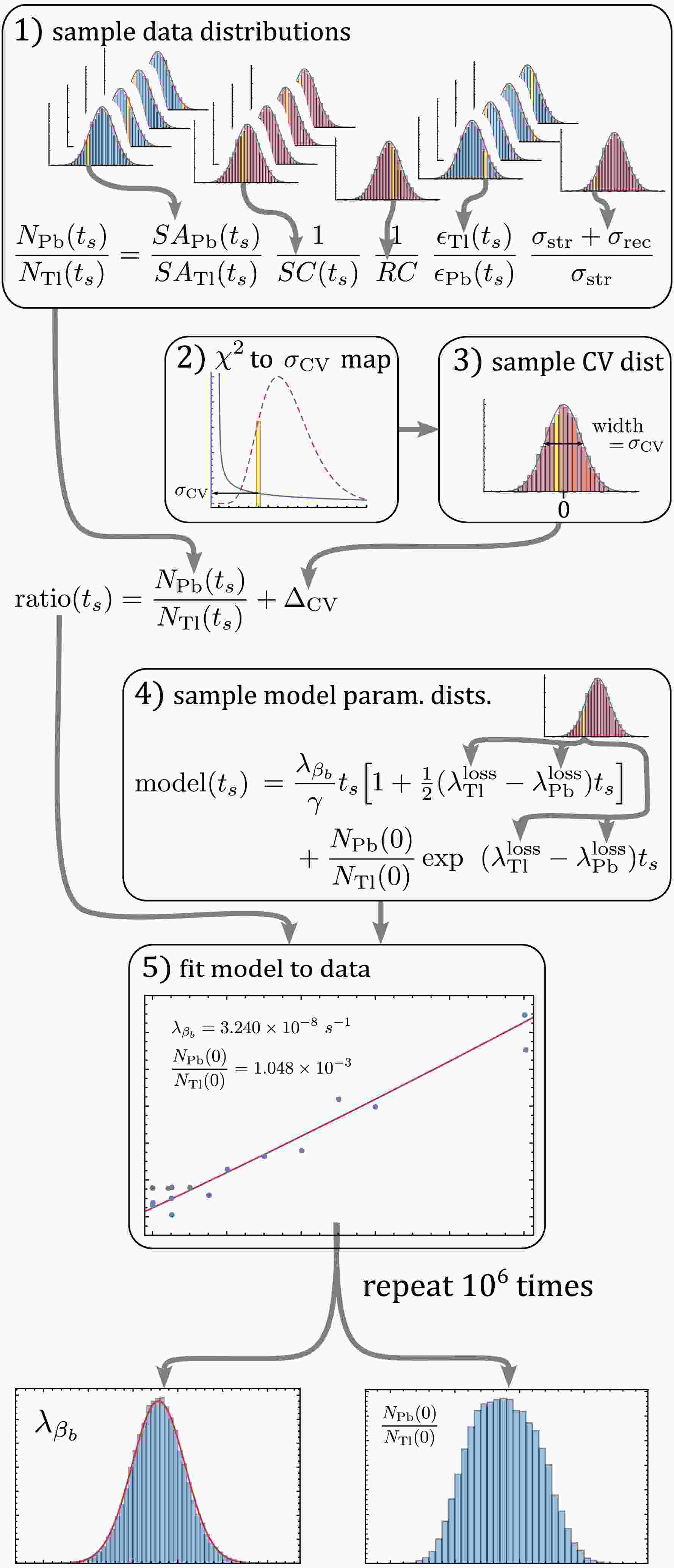(2); to fit a sampled data set with this equation, we used least squares to obtain a best fit value for the decay rate $ \lambda_{\beta_b} $. The distribution in the final model parameters is then representative of the underlying uncertainty distributions and the correlations between uncertainties, and even the "nuisance" model parameters are naturally handled by the MC simulation.

Figure 1 presents a flowchart that summarizes our implementation of the MC method, which can be broken down into five steps:

Figure 1.  (color online) A flowchart outlining the proposed MC method following the five steps described in the text. The yellow bin schematically suggests that the corresponding value was the sampled value for that MC run. The distributions in blue are uncorrelated between the 16 measurements, while distributions in red are correlated. Multiple distributions stacked indicates that the corresponding individual values were used for this variable for each of the 16 measurements, whereas a single distribution indicates a single value for all measurements.

1) Randomly sample each measured quantity (Schottky intensities, corrections, etc.) and calculate the corrected $ N_{\rm{Pb}}/N_{\rm{Tl}} $ ratio with Eq. (1) to produce 16 data points.

2) Randomly sample the $ \chi^2(\nu=14) $ distribution and determine a value for $ \sigma_{\rm{CV}} $ for that run (see discussion below for motivation).

3) Add a randomly sampled value to each data point from a Gaussian distribution with mean zero and standard deviation $ \sigma_{\rm{CV}} $ to simulate the contamination variation.

4) Randomly sample the uncertain model parameters ($ \lambda^{\rm{loss}} $ rates) to construct a model from Eq. (2) for that MC run.

5) Use least squares to fit the sampled model and obtain a best fit value for $ \lambda_{\beta_b} $ and $ N_{\rm{Pb}}(0)/N_{\rm{Tl}}(0) $.

This method was repeated 10⁶ times to produce a distribution of final model parameters. Our code for the MC method is also available publicly in Ref. [25].

The strength of the MC method is that it is straightforward to apply to an arbitrarily complex analysis while simultaneously handling correlations between inputs, even if the input uncertainties have highly unusual distributions; this was the primary motivation for our analysis. The weakness is that it is a numerical method, so the precision of the model parameter distributions is determined by the number of MC runs m, which can be a significant limitation if the analysis is computationally expensive. Typically, $ m>10^4 $ is considered sufficient, and for our relatively simple model fit, we were able to achieve a MC accuracy of 0.02% with $ m=10^6 $ MC runs.

Figure 2 shows the experimental data, with each data point representing the ratio derived at the end of a storage run with the error bars representing the "raw statistical error" derived from the median and $ \pm1\sigma $ intervals of the MC simulation for that ratio. This figure also shows the best fit results from 100 sample MC runs, with the inset showing the histogram of the MC best fit results of the $ \beta_b $ decay rate.

Figure 2.  (color online) ²⁰⁵Pb/²⁰⁵Tl ratios for all storage periods, including the "raw uncertainty" from the corrections, alongside a sample of 100 MC fits (red) and the median MC fit result (blue), which represents the median value of the MC histogram of the final model parameters. The residuals (lower panel) highlight that some statistical variation is missing to account for the scatter in the data. The inset shows the MC histogram for $ \lambda_{\beta_b} $ with the Gaussian fit used to extract the model parameter distribution.

Analyzing the residuals in Fig. 2, it is clear that the "raw uncertainty" from the corrections cannot explain the scatter in the data, indicating that not all of the experimental uncertainty was accounted for. In particular, the value of $ \chi^2 $ for the data in Fig. 2 is 303, whereas the 95% confidence interval for a $ \chi^2 $ distribution with 14 degrees of freedom is [6.6, 23.7]. The first remedy for missing uncertainty should always be the careful examination of the data and the identification and quantification of the unaccounted-for uncertainty. For this purpose, we surveyed a list of possible sources of systematic effects; the details are provided in §3.3.1 of Ref. [18]. Notably, Poisson "counting statistics" cannot account for all the missing uncertainty, providing variation at approximately the 3% level (see Sec. IV for a deeper discussion). By exclusion of all other possibilities, we concluded that this variation most likely arose from fluctuations in the field strengths of the FRS magnets between storage periods. Given the FRS-selected a $ >3\sigma $ tail from the ²⁰⁵Pb fragmentation distribution, it is likely that such fluctuations could produce the missing uncertainty of ~ 6% in the ²⁰⁵Pb contamination level that was observed.

Given that there was no method to measure this contamination variation from the FRS because it was perfectly confounded with our signal, the missing uncertainty must be quantified by analyzing the scatter in the data. While bootstrapping by random re-sampling of the data is a self-consistent method with minimal assumptions that was used in earlier stages of this analysis, our simulations have shown that it is only accurate if more than 50 data points are available. With only 16 data points, we were forced to turn to other methods.

We first considered the well-known Birge ratio method [29]. Discussed at length in a recent publication of ours [30], the Birge ratio is used to globally increase all error bars by a factor $ \tilde{\sigma}_i=R_B\,\sigma_i $ with

where n is the number of data points $ (x_i,y_i) $ being evaluated and k is the number of parameters $ \vec{\alpha} $ of the model. This has the effect of globally inflating the error bars until $ \chi^2=n-k $. However, inflating the error bars maintains their relative size, which in our case underweights the long storage time measurements that contain most of the signal from $ \beta_b $ decay. Specifically, the uncertainty coming from the corrections is much smaller for short storage times, while the contamination variation from the FRS should affect all data points equally. For this reason, we chose to add additional uncertainty $ \sigma_{\rm{CV}} $ in quadrature rather than to inflate the raw uncertainties, yielding a value of $ \chi^2 $ expressed as

Note that the contamination variation $ \sigma_{\rm{CV}} $ must be multiplied by the storage loss factor $ \exp[(\lambda^{\rm{loss}}_{\rm{Tl}}-\lambda^{\rm{loss}}_{\rm{Pb}})t_s] $ to account for the evolution of the contamination with storage time.

The Birge ratio also breaks down for small numbers of data points because the $ \chi^2 $ distribution distribution can no longer sufficiently constrain the missing uncertainty. Consider our case with $ n-k =14 $ where the 95% confidence interval of the associated $ \chi^2 $ distribution is [6.6, 23.7]. Using the Birge ratio to achieve a final $ \chi^2 $ value of 14 is not well motivated over other values in this range, which has led to criticism of the method over the years. However, this problem can be naturally solved by the Monte Carlo propagation method because for each MC run, a different target value for $ \chi^2 $ can be chosen. Specifically, we constructed a mapping between the $ \sigma_{\rm{CV}} $ value and the minimum $ \chi^2 $ value for that $ \sigma_{\rm{CV}} $ value. Using this mapping, we could then randomly sample a $ \chi^2 $ variate for that MC run and determine how much contamination variation to add to the data for that MC simulation run. This allowed us to naturally incorporate the uncertainty with which the data can constrain the missing statistical variation identified by the $ \chi^2 $ goodness of fit test, solving a key weakness of the Birge ratio through the unique framework of the Monte Carlo method. The mapping between the value of $ \chi^2 $ and $ \sigma_{\rm{CV}} $ is represented in Fig. 3 along with the $ \chi^2(\nu=14) $ probability distribution that was sampled.

Figure 3.  (color online) Mapping (in blue) between the $ \chi^2 $ variate and the estimated contamination variation $ \sigma_{\rm{CV}} $ required to achieve that value for our data and model. The $ \chi^2(\nu=14) $ probability distribution is also represented (in red) to visually convey how often a given value was sampled.

The histogram of best fit values for $ \lambda_{\beta_b} $—shown in the inset of Fig. 2—gives the final uncertainty distribution for the parameter: $ \lambda_{\beta_b}=2.76(28)\times10^{-8}\; {\rm{s}}^{-1} $, as reported in Refs. [11, 12]. This distribution includes the raw statistical error as well as the correlated systematic errors and estimated contamination variation.

Another well-known weakness of the $ \chi^2 $ minimization method is the sensitivity to possible outliers [30−32]. A single outlier can dramatically increase the calculated value of $ \chi^2 $, thus increasing the estimated missing uncertainty as well as biasing the result. We observed this effect in our data analysis as a result of the outlier tagged in the bottom-left of Fig. 2. When included in the analysis, it increased the slope of the fit and doubled the uncertainty, giving a final distribution of $ \lambda_{\beta_b}=3.13(47)\times10^{-8}\; {\rm{s}}^{-1} $. This outlier was $ 6.7\sigma $ away from the best fit prediction, even with the missing uncertainty included, so we discarded this data point for the above MC analysis. This case highlights a further weakness of using $ \chi^2 $ to estimate missing uncertainty. It must be paired with judicious data selection to provide reasonable results, which can be slow and painstaking work when done carefully.

It was quickly determined that the uncertainty arising from counting a finite number of decays, otherwise known as "counting statistics", could not explain the missing variation in our data (producing ~ 3% variation, whereas 6% was missing). Given that the variation from the counting statistics is automatically included in the estimation of the contamination variation in the MC method, we did not differentiate between these two sources in the analysis reported in Refs. [11, 12, 18, 19]. This sufficed for an accurate determination of $ \lambda_{\beta_b} $; however, as we shall see, an in-depth treatment of counting statistics is necessary to compare the MC method with a Bayesian analysis.

In a typical decay counting experiment, the impact of counting statistics is accounted for via the Poisson uncertainties on the counting bins or, ideally, via the Maximum Likelihood Estimator, where each data point is considered individually. The $ \beta_b $-decay measurements are atypical because the ions cannot be identified at the time of decay given that they are mixed with the parent ions owing to the small Q value of the decay. Thus, ions must be counted at the end of the storage period. The number of ions that decay during a given storage period follow a Poisson distribution; furthermore, the ions are affected by beam losses and the initial ion population in this experiment arose from projectile fragmentation, both of which are also Poisson processes. Fortunately, the sum of two independent Poisson variables $ X\sim P(\lambda) $ and $ Y\sim P(\eta) $ is itself a Poisson variable with $ X+Y\sim P(\lambda+\eta) $, so the Poisson variation from all of these processes is just determined by the number of ions at any given time. It is worth noting that while the parent and daughter populations are 100% correlated for radioactive decay, the loss constants $ \lambda^{\rm{loss}} $ are three orders-of-magnitude larger than $ \lambda_{\beta_b} $, so the variance of the $ N_{\rm{Tl}} $ and $ N_{\rm{Pb}} $ populations are not correlated in this experiment.

For the first two $ \beta_b $-decay experiments [4, 5], the fully-stripped $ \beta_b $-decay daughters were counted with particle detectors. Therefore, the number of ions was known immediately. For ²⁰⁵Tl⁸¹⁺, we chose to measure the ratio of Schottky noise power densities—proportional to the ion number according to the Schottky theorem—to avoid introducing systematic errors when calibrating the Schottky detectors. While the Schottky noise power density has its own uncertainty, it does not account for the variance introduced by the Poisson statistics. The Poisson uncertainty in the ratio $ R=N_{\rm{Pb}}/N_{\rm{Tl}} $ is just $ \sigma_R=\sqrt{R/N_{\rm{Tl}}} $ (see Appendix A for derivation). Using this expression, we can add Poisson uncertainty to each data point using the MC method in the same manner that we added the contamination variation. The results are shown in Fig. 4. As can be seen from the residuals, Poisson statistics alone are not enough to account for the missing uncertainty, although they do explain a third of the unaccounted-for variation. However, as expected, the final result from an updated MC analysis is $ \lambda_{\beta_b}= 2.78(30)\times 10^{-8}\; {\rm{s}}^{-1} $, almost identical to the published result, indicating that the Poisson variation had been included in the contamination variation. Despite this, explicitly modeling Poisson statistics is essential when comparing the MC method with the Bayesian analysis because we are primarily interested in the behaviour of the methods when estimating the missing uncertainty.

Figure 4.  (color online) Updated MC method with error bars indicating the variance included for Poisson statistics and updated contamination variation. The example of 100 MC fits is again represented in red with the median fit result used to calculate the residuals. The pie chart shows the contribution of each source to the total uncertainty, highlighting that the dominant uncertainty for the experiment remains the contamination variation from the FRS.

The fully Bayesian approach, similar to the previously described MC method, properly evaluates the likelihood by accounting for the uncertainty of the model parameters. For this purpose, each experimental datum was evaluated as a Gaussian probability distribution centered at the mean value with a standard deviation equal to the associated uncertainty. However, differently from the method described in the previous section, it does not simply minimize the likelihood but efficiently explores the allowed parameter space taking into account possible multimodalities. Unlike the Monte Carlo method, the dependence between data is ignored. The posterior probabilities were obtained by evaluating the likelihood function over the parameter space using the nested sampling method [33, 34] and, more specifically, the $ {\rm{\small{NESTED\_FIT}}} $ code [35−37]. The nested sampling is a recursive search algorithm using an ensemble of sampling points that evolves during the algorithm execution. It is a method normally used for Bayesian model selection in which, in addition to finding the maximum of the likelihood function, a probability for each model is evaluated from the integral over the parameter space of the model (via the calculation of the Bayesian evidence). In this study, however, the $ {\rm{\small{NESTED\_FIT}}} $ code was not used for the Bayesian model selection but only for the powerful exploration features of the nested sampling and the capability of $ {\rm{\small{NESTED\_FIT}}} $ to treat multimodal solutions and to use non-standard likelihoods.

The standard procedure builds the likelihood function by considering a normal (Gaussian) distribution of the experimental data with respect to the model value, with the mean equal to the experimental value $ y_i $ and the standard deviation equal to the value of the error bar $ \sigma_i $. The maximization of the likelihood thus corresponds to the minimization of the associated $ \chi^2 $ value. Alternatively, we considered also the approach proposed by Sivia [38], referred here to as the conservative approach, for a robust analysis. For each data point, the error bar value is instead considered as a lower bound on the real unknown uncertainty $ \sigma'_i $ that includes unevaluated systematic contributions. After marginalization over the possible values of $ \sigma'_i $ (considering a modified version of non-informative Jeffreys prior), for each datum the corresponding distribution is no longer a normal distribution but now features lateral tails decreasing as $ 1/(y - y_i)^2 $ (see Fig. 5), where $ y=y_i-f[x_i|\vec{\alpha}] $ is the theoretical expected value for the modeling function $ f[x_i|\vec{\alpha}] $. More precisely, the final likelihood function L is now given by

Figure 5.  (color online) Standard Gaussian distribution compared to the distribution derived by the Bayesian conservative method for each single data point $ y_i $ with standard deviation $ \sigma_i $.

Because of the slower drop-off at extreme values of y, such a distribution is naturally more tolerant to outliers and, more generally, to inconsistency between error bars and data dispersion.

By using the $ {\rm{\small{NESTED\_FIT}}} $ code, different estimates for the $ \beta_b $ decay constant were extracted by analyzing the same data as in Ref. [11] ("raw uncertainties") or with the Poisson statistical additional contribution discussed in Sec. IV. In addition, we considered the entire available data set ("all") with and without the outlier in the bottom-left of Fig. 2 that was excluded from the MC method. Finally, we considered both standard Gaussian and conservative distributions. The different results are presented in Fig. 6. For all different cases, the uncertainties of the parameters $ \lambda^{\rm{loss}}_{\rm{Tl}} $ and $ \lambda^{\rm{loss}}_{\rm{Pb}} $ were taken into account by considering Gaussian prior probabilities with the parameter uncertainty as standard deviation (and its nominal value as mean). Owing to the very small relative uncertainty ($10^{-3} $), no priors were considered for $ \gamma $, which is considered as exact. Slice sampling [39] was used for the search of the sampling points in $ {\rm{\small{NESTED\_FIT}}} $because of its superior performance with respect to other methods (for example, random walk; see [37]). Typical computation times were in the order of a few seconds on a standard laptop PC.

Figure 6.  (color online) Comparison between the different statistical analysis. The grey band corresponds to the reported value in [11]. The other approaches, indexed in the legend with three possible variations, are described in the text.

As expected, the presence of outliers significantly introduces bias in determining the decay constant when the standard likelihood is used, even when considering uncertainty evaluations from the Poisson statistics of the ions. Once the outlier is excluded, the obtained decay value is consistent with the MC method reported in Ref. [11], where the uncertainties were globally increased to justify the residual scattering.

When the conservative method is adopted, no difference is observed whether the outlier is included or not, demonstrating the robustness of the method. However, the corresponding uncertainties are larger than in the other cases because the conservative method assumes missing systematic uncertainty contributions for each data point. It is notable that, for the conservative method, even if the error bars of the raw data are underestimated, the final evaluation of the decay constant is close to the value obtained by eliminating the outlier and artificially inflating the error bars using the Monte Carlo method discussed in Sec. III (grey band in Fig. 6). The use of a more tolerant probability distribution (Fig. 5) leads, in fact, to a final uncertainty that depends on the data dispersion. This is not completely the case for standard $ \chi^2 $ minimization methods. See Ref. [30] for a more extended discussion on this aspect, but applied to weighted averages. Among the different approaches, the preferable option is the one with the least working hypotheses considering the best of our possible knowledge at present. This corresponds to considering the entire set with the Poisson statistics uncertainty resulting in the parameter estimate of $ \lambda_{\beta_b}= 2.62(32)\times 10^{-8}\; {\rm{s}}^{-1} $.

As seen in the previous sections, the different robust statistical approaches reassuringly yield very similar results, even when the statistical uncertainty is underestimated.

The Monte Carlo method is a robust technique for handling underestimated uncertainties in small data sets while respecting the uncertainty in the ability of the data to constrain the missing uncertainty, namely the fluctuation in the $ \chi^2 $ distribution. Simultaneously, it takes into account correlations in the data and uncertainties in the nuisance parameters of the model, making it a flexible tool. An outstanding weakness is that outlier detection must be done manually to ensure an accurate estimate of the missing uncertainty.

The Bayesian method is simpler in that it requires fewer assumptions about the data. Taking advantage of the Bayesian framework, uncertain parameters can be represented with experimentally determined prior distributions, and that uncertainty is naturally incorporated when these parameters are integrated out in the final estimation. The implemented missing uncertainty estimation is also optimized to handle outliers, making it a very flexible tool. However, correlations between data points cannot be considered in the current likelihood construction. This does not appear to be a limitation in this analysis, as the uncertainty is dominated by uncorrelated contamination variation and Poisson counting statistics.

The two methods produce remarkably consistent results, as shown in Fig. 6, especially when considering they handle the missing uncertainty in a fundamentally different manner. The MC method adds the same additional uncertainty to all data points, scaling the entire data set together. This is appropriate if the unknown variation affects all data points equally and has the advantage of not treating any data point preferentially, though it reduces the constraining power of the more precise points. The Bayesian method, on the other hand, treats the missing uncertainty for each data point individually. This optimizes the Bayesian method to handle outliers but also allows for situations where the minimization may allow for several optimising parameter values sets.

The estimation of unknown statistical error is a common challenge in experimental physics, and while every effort should be made to fully understand the uncertainties of an experiment, sometimes sources of uncertainty must be estimated from the data itself. The method used to estimate this missing uncertainty should be as accurate and unbiased as possible. One of the most common methods for estimating missing uncertainty has been the Birge ratio. However, we have explained how it is biased towards the most probable $ \chi^2 $ of the data and does not take into account the full range of possibilities for model parameters that are compatible with the data. We have presented two methods that provide an alternative to the Birge ratio. The Monte Carlo method takes advantage of the fact that it uses multiple trials, so the $ \chi^2 $ value that is replicated can be varied with each trial. The Bayesian method takes advantage of the fact that Bayesian analysis can self-consistently allow the data to constrain the missing uncertainty. As a result, both of these methods improve on the traditional Birge ratio and more reliably represent the uncertainty of the measured parameters.

The application of multiple analysis methods also provides a useful assessment on the variation in our final value and uncertainty. We have shown here that across a broad range of analysis methods, our final result for the $ \beta_b $ decay rate is reliable and features a very reproducible uncertainty. A correct treatment of the Poisson statistics improves the coherence of the results by decomposing the missing uncertainty into its Poisson and contamination variation components explicitly. It is also reassuring to note that this dedicated analysis resulted in only a 0.7% or $ 0.07\sigma $ increase on the final value reported in Refs. [11, 12]. Once counting statistics are included, which is essential for a fair comparison, the MC and Bayesian methods agree on the reported value within $ 0.5\sigma $ and provide almost identical estimates for the size of the parameter uncertainty. This highlights the remarkable robustness of our reported half-life value considering how different the methods are.

The presence of the outlier (bottom-left in Fig. 2) also tested the ability of the method to handle outliers. The Bayesian method is clearly better suited to handle outliers because the missing uncertainty is evaluated individually for each data point, allowing individual outliers to be inflated without penalizing the entire data set. The fact that the method can handle both the outlier and missing uncertainty out-of-the-box and yield a similar result to that from the MC method, which required months of work to perfect, demonstrates its versatility and reliability in analyzing challenging data. As a result, we recommend the use of the open-source $ {\rm{\small{NESTED\_FIT}}} $ code [35−37] for future experimental analysis. For those who require an alternative to Bayesian methods, which can be sometimes computational costly, or when strong correlations in the data exist, we also recommend the Monte Carlo method for easy error propagation and as a natural mechanism for estimating missing uncertainty.

The results presented here are based on the experiment G-17-E121, which was performed at the FRS-ESR facilities at the GSI Helmholtzzentrum für Schwerionenforschung, Darmstadt (Germany) in the frame of FAIR Phase-0.

To estimate the contribution of counting statistics to our final data points, we aim to calculate the variance of our ratio data points arising from the underlying Poisson variables. Noting that the variance of a Poisson distribution is equal to its mean, the definition of the ratio $ R=N_{\rm{Pb}}/N_{\rm{Tl}} $ implies that the variance of R is given by

Given that $ R\ll1 $ in our case, we have that $ {\rm{Var}}(R)\approx R/N_{\rm{Tl}} $. Note that because we only measured the ratio via Schottky detectors and $ N_{\rm{Tl}} $ by the DC current transformer [11, 12], we have expressed Var(R) just in terms of these variables.