Testing redshift variation in the X-ray and ultraviolet luminosity relations of quasars

Quasars (quasi-stellar objects) are extremely luminous and persistent sources powered by gas spiraling at high velocity into supermassive black holes. Their immense luminosity, often thousands of times greater than that of the Milky Way, makes them visible across vast cosmological distances. The maximum observed redshift of quasars fulfills $ z>7 $ [1−4]. To date, more than half a million quasars have been identified. Quasars serve as reliable cosmological probes, offering a valuable tool for filling the redshift desert in observational data. Consequently, they have been widely utilized to investigate the nature of dark energy, explore the potential origins of the Hubble constant ($ H_0 $) tension, test the cosmic distance duality relation [5], and other purposes.

In quasar cosmology, establishing a robust luminosity relation is essential for determining quasar distances. Several empirical relations have been proposed, including the anticorrelation between ultraviolet (UV) emission lines and luminosity [6, 7], luminosity-mass relation in super-Eddington accreting quasars [8], relation between luminosity and X-ray variability [9], radius-luminosity relationship [10−12], redshift-angular size relation [13−18], and nonlinear relation between X-ray luminosity ($ L_\mathrm{X} $) and UV luminosity ($ L_\mathrm{UV} $) [19−22]. The $ L_\mathrm{X} $-$ L_\mathrm{UV} $ relation has gained particular prominence in constructing the Hubble diagram of quasars, extending to redshifts as high as $ z\sim 7.5 $ [23−31]. The cosmological distance can be derived from the Hubble diagram. Initially, the results fit the cosmological constant plus the cold dark matter (ΛCDM) model well and match distances inferred from type-Ia supernova (SN Ia) [21]. However, several groups found recently that the distance modulus/redshift relation of quasars derived from the $ L_\mathrm{X} $-$ L_\mathrm{UV} $ relation has an apparent deviation from the prediction of the ΛCDM model [23, 32−35]. This deviation raises concerns about the accuracy of the $ L_\mathrm{X} $-$ L_\mathrm{UV} $ relation and suggests that it may evolve with redshift [36].

The potential redshift evolution of the $ L_\mathrm{X} $-$ L_\mathrm{UV} $ relation has been explored in prior studies [37, 38] although these analyses present limitations. For example, Wang et al. [37] divided a quasar sample into low-redshift ($ z<1.4 $) and high-redshift $ z>1.4 $ subsets and found that the relation coefficients for the two subsamples differ by more than $ 2\sigma $. Similarly, Li et al. [38] split a quasar sample with $ z<2.261 $ into two parts with approximately the same data number ($ \langle z \rangle=1.16 $) and found similar deviations between the relation coefficients. While it is now recognized that the relation coefficients vary across redshift ranges, their precise evolutionary behavior remains unclear.

Recently, a three-dimensional and redshift evolutionary $ L_\mathrm{X} $-$ L_\mathrm{UV} $ relation has been constructed in [39]; it is based on a redshift-dependent correction to the luminosities of quasars. Additionally, Wang et al. [37] applied the statistical tool copula [40] to construct another three-dimensional and redshift evolutionary $ L_\mathrm{X} $-$ L_\mathrm{UV} $ relation. Subsequent analyses have indicated [41, 42] that the copula-based relation outperforms both the standard $ L_\mathrm{X} $-$ L_\mathrm{UV} $ relation and the relation given in [39]. However, whether these generalized relations fully eliminate redshift variations in the relation coefficients requires further scrutiny.

Thus, in this study, we systematically tested the redshift dependence of both two- and three-dimensional $ L_\mathrm{X} $-$ L_\mathrm{UV} $ relations. The paper is organized as follows. In Sec. II, we examine the redshift variation of the standard $ L_\mathrm{X} $-$ L_\mathrm{UV} $relation. In Sec. III, we investigate whether the selection effect results in the redshift variation of the $ L_\mathrm{X} $-$ L_\mathrm{UV} $ relation. In Sec. IV, we analyze two three-dimensional $ L_\mathrm{X} $-$ L_\mathrm{UV} $ relations. We propose a new $ L_\mathrm{X} $-$ L_\mathrm{UV} $ relation in Sec. V. Finally, in Sec. VI, we summarize our findings.

The standard $ L_\mathrm{X} $-$ L_\mathrm{UV} $ relation describes a non-linear relationship between the X-ray and UV luminosities of quasars [19−22]; it takes the form

where $ L_\mathrm{X} $ and $ L_\mathrm{UV} $ are the luminosities (in $ \mathrm{erg\; s}^{-1}\; \mathrm{Hz}^{-1} $) at 2 keV and 2500 $ \mathring{A} $, respectively, and β and γ are two relation coefficients. Converting luminosity to flux, we obtain

where $ F_\mathrm{X}=\dfrac{ L_\mathrm{X}}{4\pi d_L^2} $ and $ F_\mathrm{UV}=\dfrac{ L_\mathrm{UV}}{4\pi d_L^2} $ are the fluxes of the X-ray and UV, respectively, and $ d_L $ is the luminosity distance, which depends on cosmological models.

Thus, given a cosmological model, the values of relation coefficients and the intrinsic dispersion of quasars can be determined from the observed quasar data. In this study, we chose the cosmological model to be a spatially flat ΛCDM model with $ H_0=70\; {\mathrm{km\; s^{-1}\; Mpc^{-1}}} $ and $ {\mathrm{\Omega_{m0}}}= $ 0.3, where $ {\mathrm{\Omega_{m0}}} $ is the present dimensionless matter density parameter.

The data sample of quasars used in our analysis consists of 2421 X-ray and UV flux measurements, spanning a redshift range from $ z = 0.009 $ to 7.541 [26]. These sources were carefully selected from an initial sample of 21,785 data points based on several criteria for the X-ray and ultraviolet bands, including signal-to-noise ratio, host galaxy contamination in the ultraviolet band, X-ray absorption, and Eddington bias. These criteria were chosen to minimize observational biases. Using the maximum likelihood estimation method [43], we obtained $ \beta=6.298\pm 0.228 $ and $ \gamma=0.665\pm0.007 $ as well as an intrinsic dispersion $ \delta=0.230\pm0.004 $ from the 2421 quasar data points.

To test whether the $ L_\mathrm{X} $-$ L_\mathrm{UV} $ relation varies with cosmological redshift, we separated the 2421 quasars into four groups based on their redshift and calculated the mean redshift for each group. The four groups, which have almost equal data numbers and cover the redshift range from low to high values, are described as follows:

● Group 1 – 606 quasars, $ 0.009\leq z <0.844 $, $ \langle z \rangle=0.586 $

● Group 2 – 605 quasars, $ 0.844\leq z <1.298 $, $ \langle z \rangle=1.064 $

● Group 3 – 605 quasars, $ 1.298\leq z<1.892 $, $ \langle z \rangle=1.578 $

● Group 4 – 605 quasars, $ 1.892\leq z\leq7.541 $, $ \langle z \rangle=2.561 $

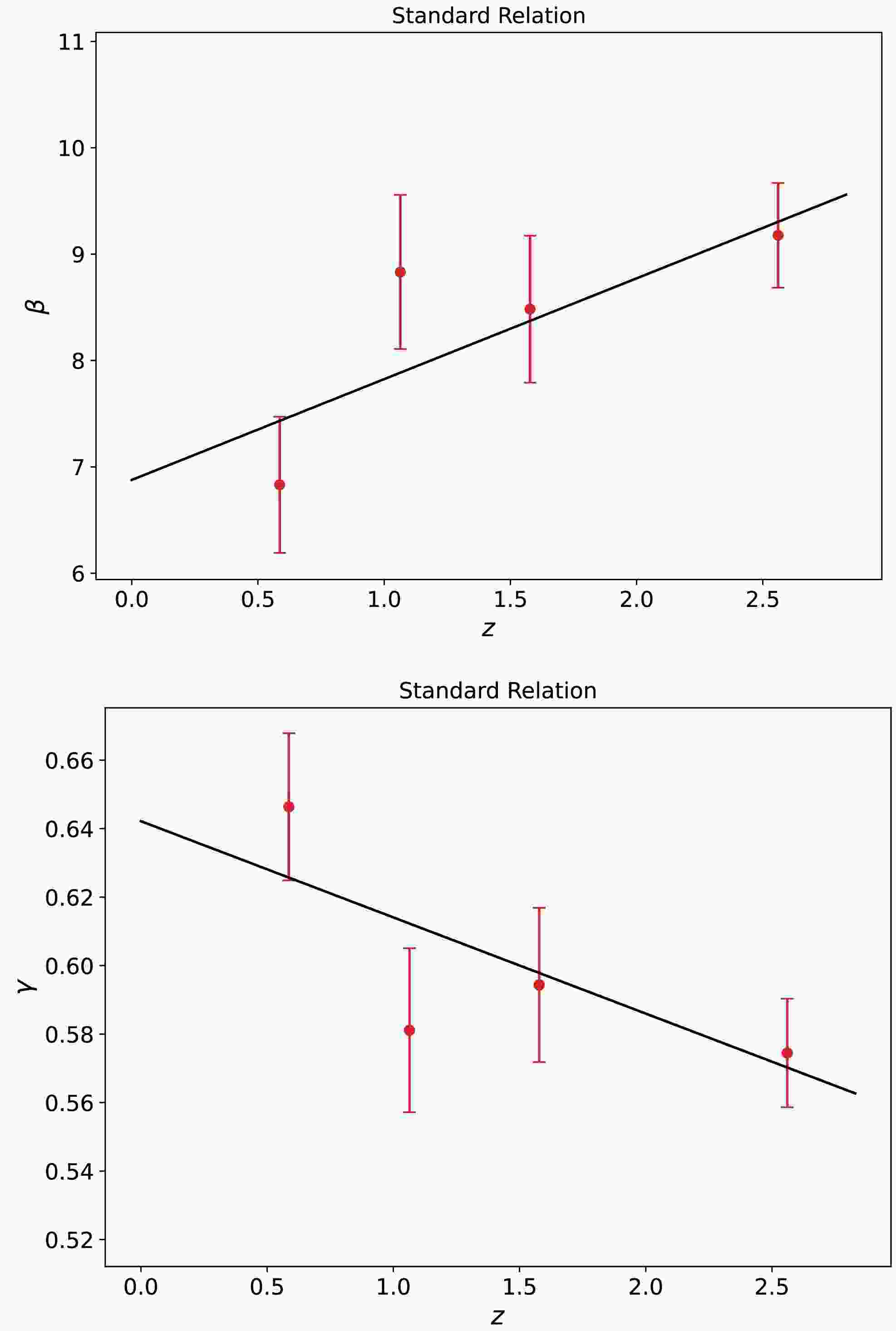
Then, we compared the data in each group with Eq. (1) and checked whether the values of β and γ evolve with redshift. Utilizing the maximum likelihood estimation method [43] to fit each group of quasars, we obtained ($\beta= 6.831\pm 0.640$, $ \gamma=0.646\pm0.021 $) for Group 1, ($\beta=8.832\pm 0.724$, $ \gamma=0.581\pm0.024 $) for Group 2, ($ \beta=8.482\pm0.691 $, $\gamma= 0.594\pm0.022$) for Group 3, and ($ \beta=9.177\pm0.492 $, $ \gamma=0.574\pm0.016 $) for Group 4. The corresponding results are shown in Fig. 1. Note that as $ \langle z \rangle $ increases, β increases approximately linearly, and γ decreases linearly. This means that β and γ are strongly correlated/anticorrelated with $ \langle z \rangle $. We used a linear function to fit β-$ \langle z \rangle $ and γ-$ \langle z \rangle $, obtaining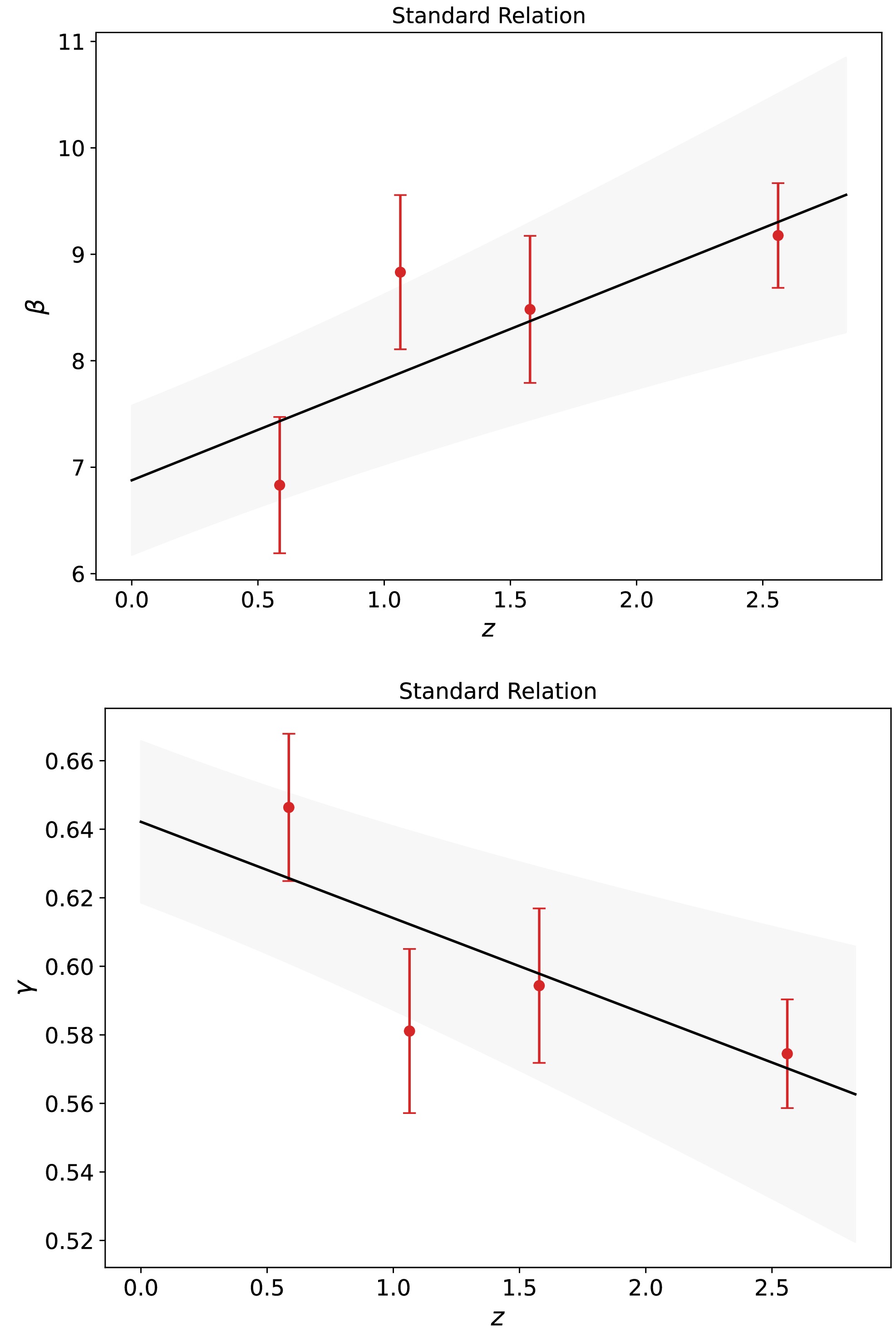

Figure 1.  (color online) Values of β and γ as a function of the mean redshift of quasars. Each data point with 1σ error bars represents a group of quasars (1, 2, 3, and 4). The solid line represents a linear fit.

and

These results show that parameters β and γ tend to evolve with redshift, given that the slopes of these relationships deviate from zero by more than $ 2\sigma $ confidence level (CL).

To minimize the impact of grouping strategies on the redshift evolution trends in the luminosity relation coefficients, we also divided the quasar sample into four groups with equal redshift intervals:

● Group 1 – 460 quasars, $ 0.009\leq0.750 $, $ \langle z \rangle=0.520 $

● Group 2 – 959 quasars, $ 0.750\leq1.500 $, $ \langle z \rangle=1.095 $

● Group 3 – 644 quasars, $ 1.500\leq2.250 $, $ \langle z \rangle=1.817 $

● Group 4 – 263 quasars, $ 2.250\leq3.000 $, $ \langle z \rangle=2.529 $

We excluded quasars with redshifts exceeding 3 given that only 95 data points fall within this range. We used the maximum likelihood estimation method to fit each group of data separately, obtaining ($ \beta=6.450\pm0.718 $, $ \gamma=0.659\pm 0.024 $) for Group 1, ($ \beta=8.165\pm0.532 $, $ \gamma=0.603\pm0.018 $) for Group 2, ($ \beta=10.104\pm0.595 $, $ \gamma=0.542\pm0.019 $) for Group 3, ($ \beta=8.703\pm0.837 $, $ \gamma=0.590\pm0.027 $) for Group 4. The corresponding linear relations for $ \beta-\langle z \rangle $ and $ \gamma-\langle z \rangle $ are expressed as follows:

and

Clearly, the slopes of these relations remain significantly different from zero at more than 2σ CL, consistent with the results expressed by Eqs. (3), (4). Therefore, employing different grouping strategies does not change the redshift evolution trends of the parameters β and γ.

To check whether the evolutions of β and γ with redshift originate from the selection effect in the measurement process, we followed the method in [44] to generate a sample of quasars by using Monte-Carlo simulations. Given that the observed quasars provide only X-ray and UV fluxes (i.e., $ \log F_\mathrm{UV} $ and $ \log F_\mathrm{X} $), we first calculated their luminosities as $ \log L_\mathrm{UV}(\log L_\mathrm{X})=$ $\log F_\mathrm{UV}(\log F_\mathrm{X})+ \log 4\pi d_L(z)^2$ in the framework of a flat ΛCDM model with $ H_0=70\; {\mathrm{km\; s^{-1}\; Mpc^{-1}}} $ and $ {\mathrm{\Omega_{m0}}}=0.3 $. Using the real sample of 2421 quasars, we then modeled the distributions of redshift, $ \log L_\mathrm{UV} $, and measurement errors $ \sigma_\mathrm{UV} $ of quasars, respectively. It has previously been demonstrated that the quasar redshift follows a Gamma distribution [37] described by $f(z) = \dfrac{b^a z^{a-1} {\rm e}^{-b z}}{\Gamma(a)}$, with $ a=3.036 $ and $ b=2.098 $. Therefore, we used this Gamma distribution to generate the redshifts for mock quasars. Additionally, the distribution of $ \sigma_\mathrm{UV} $ was modeled as a Lognormal distribution given by $f(\sigma_\mathrm{UV}) = \dfrac{1}{\sqrt{2\pi} s\: \sigma_\mathrm{UV}} \times \exp\left\{ -\dfrac{(\log \sigma_\mathrm{UV} - \mu)^2}{2 s^2} \right\}$, with $ \mu=-4.342 $ and $ s=0.566 $; this distribution was derived directly from the real quasar data employing the Python package scipy.stats. The distribution of $ \log L_\mathrm{UV} $ is Gaussian, with a mean value of $ 30.428 $ and a standard deviation of $ 0.658 $, also derived from real data. Although observational limitations (e.g., flux detection thresholds or Eddington bias) could introduce deviations from the Gaussian assumptions for the UV luminosity, we verified the validity of this assumption through a statistical distribution test, specifically the Cramér-von Mises test [45, 46]. Then, we sampled the mock datasets of (z, $ \log L_\mathrm{UV} $, $ \sigma_\mathrm{UV} $) from these distributions. Note that we assumed no correlations between the distributions, meaning that they are mutually independent. We then introduced a UV luminosity cutoff by removing mock data with $ \log L_\mathrm{UV}<\log L_\mathrm{UV,min} $, where $ \log L_\mathrm{UV,min}= \log F_\mathrm{UV,min}+ \log 4\pi d_L(z)^2 $, with $ \log F_\mathrm{UV,min}= -28.759 $ being the minimum observable flux. For each triplet (z, $ \log L_\mathrm{UV} $, $ \sigma_\mathrm{UV} $), we sampled $ \log L_\mathrm{X} $ from the probability distribution function $ f(\log L_\mathrm{X}) = \dfrac{1}{\sqrt{2\pi}\sigma} \times \exp \left\{ -\dfrac{(\log L_\mathrm{X} - \beta - \gamma \log L_\mathrm{UV})^2}{2\sigma^2}\right\}, $ where the intrinsic dispersion σ and coefficients β and γ were fixed to $ \sigma = 0.230 $, $ \beta = 6.298 $, and $ \gamma=0.665 $, according to the calculations presented in the previous section. The mock observed error $ \sigma_\mathrm{X} $ was also sampled by assuming a Lognormal distribution with mean and standard deviation of $ -3.159 $ and $ 0.769 $, respectively, obtained from real data. After imposing an X-ray luminosity limit, analogous to the UV cutoff, by using $ \log F_\mathrm{X,min}=-32.706 $, we ultimately obtained the simulated quasar data set (z, $ \log L_\mathrm{UV} $, $ \sigma_\mathrm{UV} $, $ \log L_\mathrm{X} $, $ \sigma_\mathrm{X} $).

We could then generate 2421 simulated quasars following the above simulation process, as shown in Fig. 2. Dividing the simulated data into four groups with approximately the same number of data in each group, we could estimate the values of β and γ for each group and derive the $ \beta-\langle z \rangle $ and $ \gamma-\langle z \rangle $ relations, similar to the previous section. By repeating this process 1000 times, we derived 1000 slope pairs (${{\rm d}\beta}/{{\rm d}z}$ and ${{\rm d}\gamma}/{{\rm d}z}$) from linear fits of the coefficients. The distributions of ${{\rm d}\beta}/{{\rm d}z}$ and ${{\rm d}\gamma}/{{\rm d}z}$ are presented as a contour plot in Fig. 3, in which the results from the real data are represented by dashed lines. Note that the values of ${{\rm d}\beta}/{{\rm d}z}$ and ${{\rm d}\gamma}/{{\rm d}z}$ from the real data deviate from those from the mock data at more than $ 1\sigma $ CL. Clearly, the simulated data do not support the redshift evolution of the $ L_\mathrm{X} $-$ L_\mathrm{UV} $ relation given that both ${{\rm d}\beta}/{{\rm d}z}$ and ${{\rm d}\gamma}/{{\rm d}z}$ are consistent with zero within $ 1\sigma $ CL.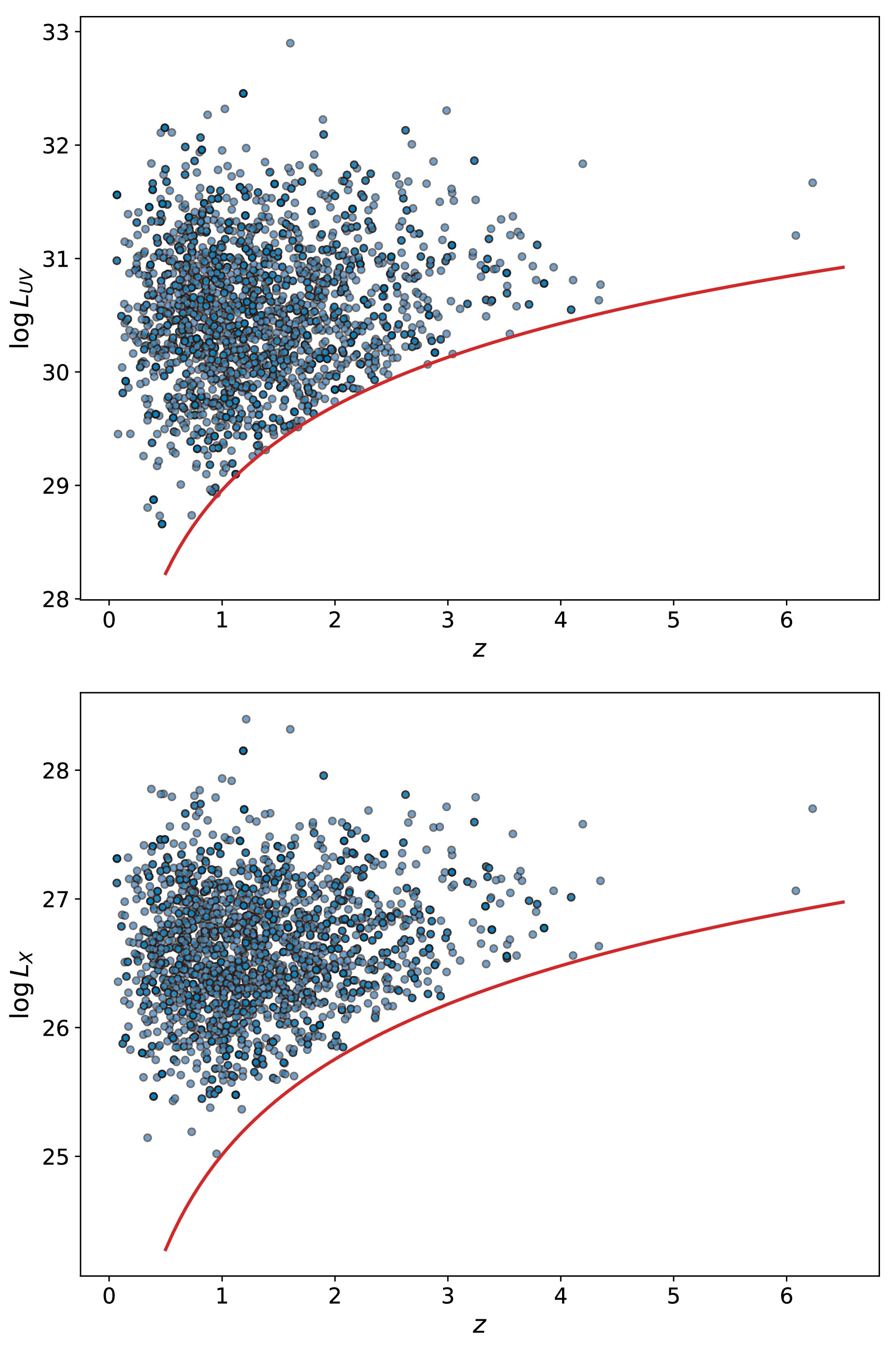

Figure 2.  (color online) Simulated $ \log L_\mathrm{UV} $ and $ \log L_\mathrm{X} $ versus redshift of quasars from the simulation method described in Sec. III.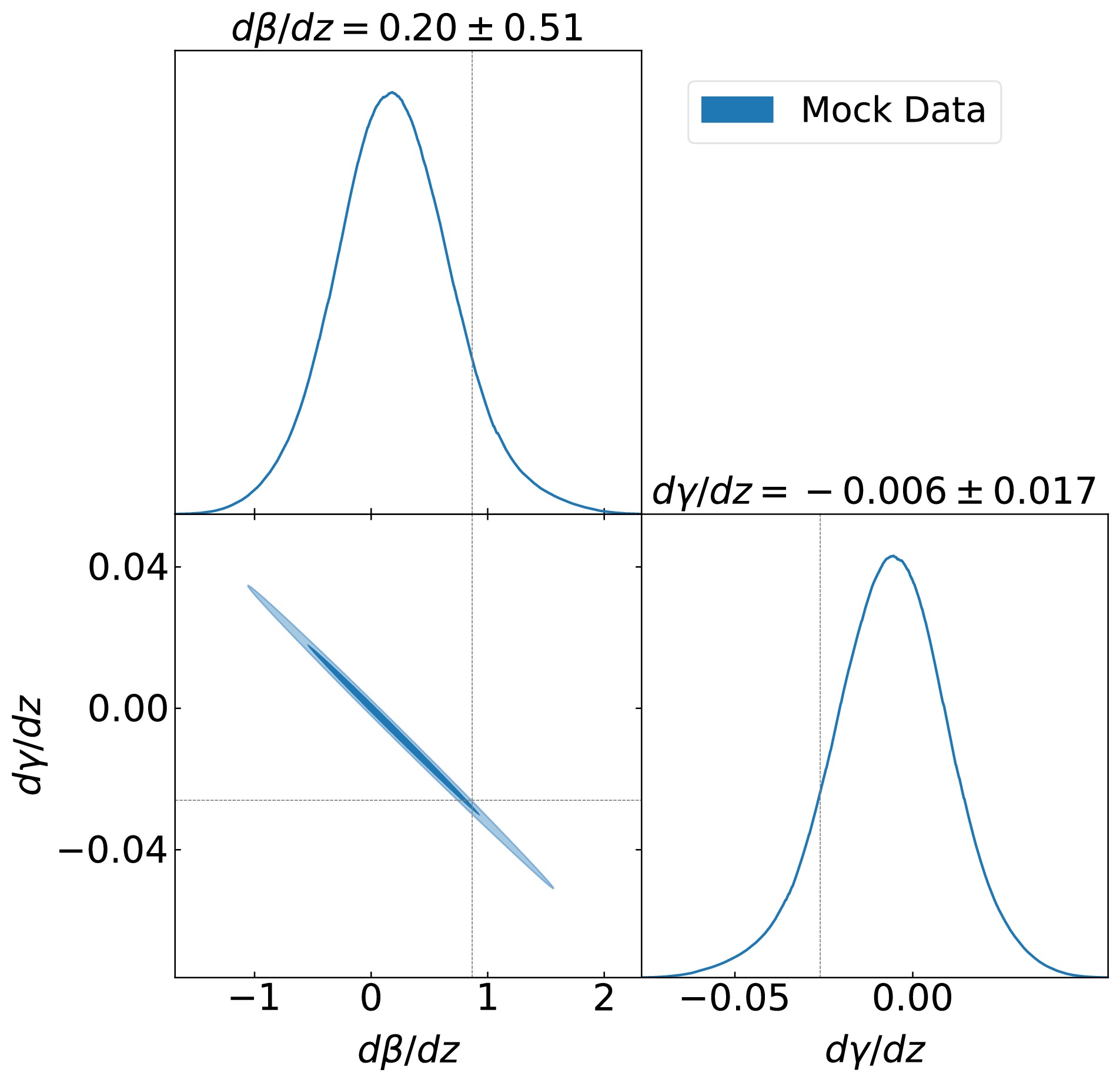

Figure 3.  (color online) Distribution of 1000 slope coefficients (${{\rm d}\beta}/{{\rm d}z}$ and ${{\rm d}\gamma}/{{\rm d}z}$) calculated from the simulated quasars; the dashed lines represent the mean values from 2421 real quasars.

To further investigate the relation between the selection effect and the redshift evolutions of β and γ, we introduced a redshift-dependent correction term $ (1+z)^k $ to adjust the luminosity [39], e.g., $ L_\mathrm{corrected}=L_\mathrm{observed}/(1+z)^k $. We then applied the Efron-Petrosian (EP) method [47] to determine the value of the parameter k. This analysis was performed using a publicly available Mathematica code: Selection biases and redshift evolution in relation to cosmology ¹. If the values of k derived from real data are significantly larger than those from mock data, it indicates that the selection effect alone cannot fully account for the redshift evolutions of β and γ. We obtained $ k_\mathrm{UV}=3.632^{+0.069}_{-0.068} $ and $ k_\mathrm{X}=2.689\pm0.053 $ for real data and $ k_\mathrm{UV}=0.106^{+0.097}_{-0.130} $ and $ k_\mathrm{X}=0.460\pm0.087 $ for mock data. Clearly, the values of $ k_\mathrm{UV} $ and $ k_\mathrm{X} $ obtained from real data are substantially larger than those from mock data, meaning that the evolutions of β and γ with redshift derived from real data cannot be attributed solely to the selection effects. This result is compatible with those presented in Fig. 3.

Let us now consider two redshift evolutionary $ L_\mathrm{X} $-$ L_\mathrm{UV} $ relations expressed in the unified form:

with $ a=1 $ and $ a=5 $, respectively. Here, α is a new parameter characterizing the redshift-dependent property of the relation, and $ \alpha=0 $ corresponds to the case of the standard relation. When $ a=1 $, this relation is obtained by assuming that the luminosities of quasars are corrected by a redshift-dependent function $ (1 + z) ^\alpha $, as in [39]. Substituting the corrected luminosities, namely, $ L_\mathrm{corrected: UV}= L_\mathrm{UV}/(1+z)^{k_\mathrm{UV}} $ and $ L_\mathrm{corrected: X}= L_\mathrm{X}/(1+z)^{k_\mathrm{X}} $, into Eq. (1) yields the relation shown in Eq. (7) for $ a=1 $. For $ a=5 $, the relation is constructed using the Gaussian copula, as in [37]. Copula is a powerful tool used to describe the correlations among $ L_\mathrm{UV} $, $ L_\mathrm{X} $, and z. Assuming that both $ \log L_\mathrm{UV} $ and $ \log L_\mathrm{X} $ follow Gaussian distributions and the redshift of quasars also follows a Gaussian distribution in the $ z_* $ space, with $ z_*=\ln (a+z) $, we constructed the relation expressed by Eq. (7). Wang et al. found that setting $ a = 5 $ provides an optimal fit after comparing results for different values of a [37].

Next, we checked whether β, γ, and α evolve with redshift. Using the observed data of quasars, we calculated their values for each group; the corresponding results are shown in Fig. 4. Note that the relation coefficients vary noticeably with redshift even when the redshift evolutionary relations are considered. The evolutionary trends of β and γ are notably similar to those shown in Fig. 1, where the standard $ L_\mathrm{X} $-$ L_\mathrm{UV} $ relation is considered. Thus, we conclude that the redshift evolutionary $ L_\mathrm{X} $-$ L_\mathrm{UV} $ relations constructed in [37, 39] are not effective in eliminating the redshift evolution of the relation coefficients.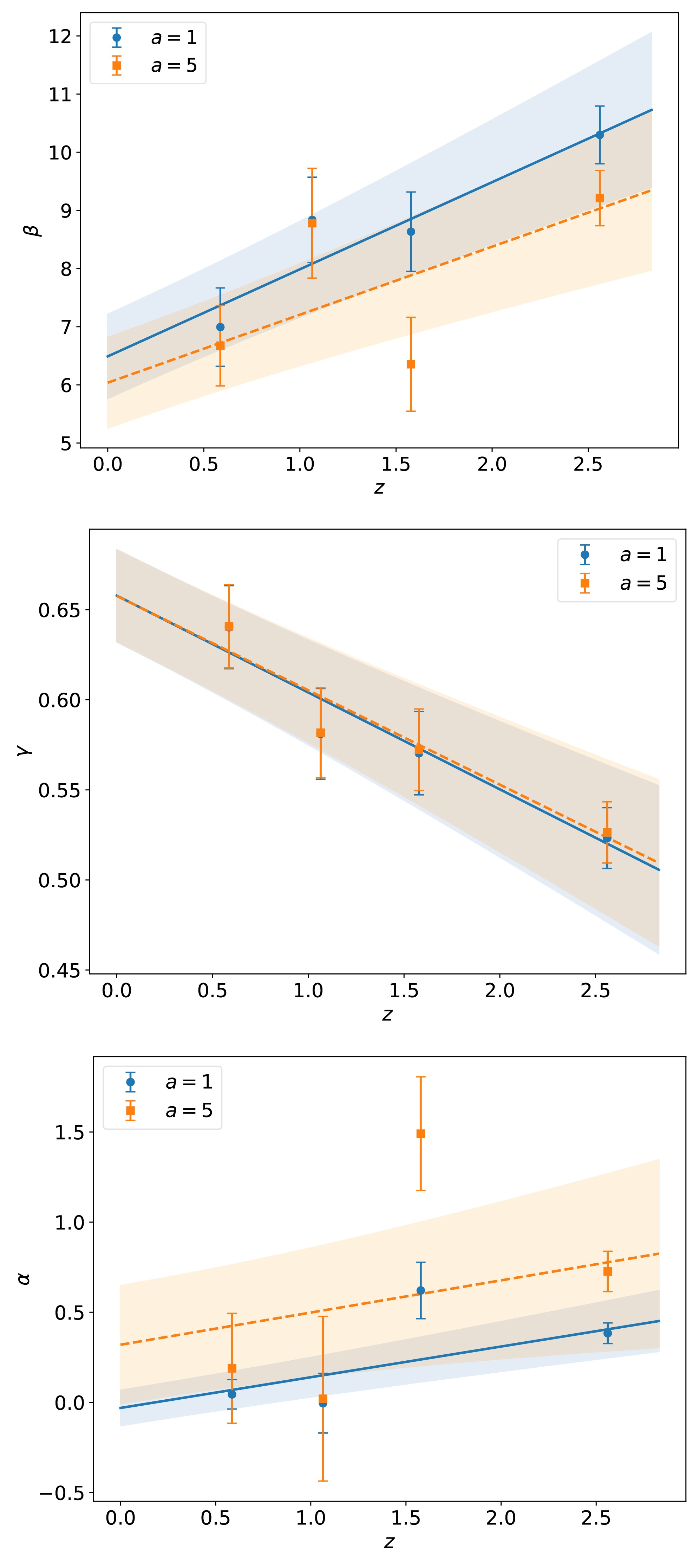

Figure 4.  (color online) Values of β, γ, and α as functions of the mean redshift of quasars based on the redshift evolutionary $ L_\mathrm{X} $-$ L_\mathrm{UV} $ relation (Eq. (7)). Each data point with 1σ error bar represents a group of quasars (1, 2, 3, and 4). The blue and orange points represent different choices for a. The lines with shaded regions represent the linear fit with 1σ uncertainty.

We have established that the standard and two redshift evolutionary $ L_\mathrm{X} $-$ L_\mathrm{UV} $ relations evolve with redshift. In this section, we aim to construct a new $ L_\mathrm{X} $-$ L_\mathrm{UV} $ relation that eliminates the redshift evolution effect. As shown in Fig. 1, coefficients β and γ depend linearly on redshift, which motivates us to propose the following relation:

where $ \tilde{\beta} $ and $ \tilde{\gamma} $ are new parameters introduced to account for any potential redshift evolution in the coefficients. This functional form is similar to the one proposed in [38]. We used real data to constrain β, γ, $ \tilde{\beta} $, and $ \tilde{\gamma} $ in the ΛCDM model with $ \Omega_\mathrm{m0}=0.3 $. The results of our analysis are shown in Fig. 5. Note that coefficients $ \tilde{\beta} $ and $ \tilde{\gamma} $ exhibit significant deviations from zero, exceeding 3σ CL, indicating that the quasar data strongly support the redshift evolutionary relation.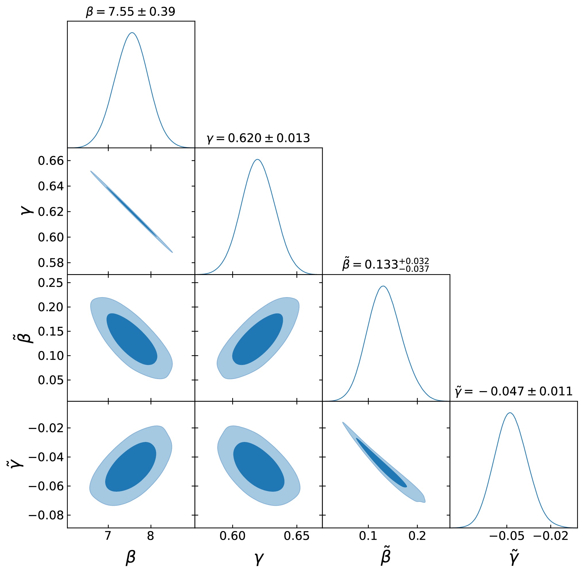

Figure 5.  (color online) Constraints on coefficients (β, γ, $ \tilde{\beta} $, and $ \tilde{\gamma} $) for the new $ L_\mathrm{X} $-$ L_\mathrm{UV} $ relation (Eq. (8)) from 2421 quasar data points in the framework of the ΛCDM model with $ \Omega_{m0}=0.3 $. The title in each subplot shows the mean value with 1σ uncertainty.

We then proceeded to constrain the values of the coefficients from four subsamples of quasars featuring approximately the same data number. We obtained

after applying a linear fit. These coefficients exhibit weak dependence on redshift, as indicated by the slope values of (${{\rm d}\beta}/{{\rm d}z}$ and ${{\rm d}\gamma}/{{\rm d}z}$), both of which are consistent with zero at $ 1\sigma $ CL. Next, given that the new $ L_\mathrm{X} $-$ L_\mathrm{UV} $ relation introduces two additional parameters compared to the standard one, we further constrained the values of β and γ by fixing $ \tilde{\beta}=0.133^{+0.032}_{-0.037} $ and $ \tilde{\gamma}=-0.047\pm 0.011 $, which are given by all quasars in the framework of the ΛCDM model. The resulting fits yield the following expressions:

Clearly, β and γ evolve very weakly with redshift given that slopes ${{\rm d}\beta}/{{\rm d}z}$ and ${{\rm d}\gamma}/{{\rm d}z}$ are consistent with zero within $ 1.5\sigma $ CL.

These results show that the new $ L_\mathrm{X} $-$ L_\mathrm{UV} $ relation effectively eliminates the redshift evolution effect on the relation coefficients. This new formulation provides a more stable and redshift-independent framework for modeling the $ L_\mathrm{X} $-$ L_\mathrm{UV} $ relation in quasars.

To investigate the effect of this new relation on the constraints of cosmological parameters, we fit the flat ΛCDM and flat wCDM models using quasars with the standard $ L_\mathrm{X} $-$ L_\mathrm{UV} $ relation and with the newly proposed relation in Eq. (8), respectively. We used Hubble parameter measurements to calibrate the luminosity relations of quasars. We also used the Gaussian Process (GP) method [48−51] to reconstruct the $ H(z) $ function from 32 observational data points spanning a redshift range of $ 0.07 \leq z \leq 1.965 $ [52]. The reconstructed result is shown in the upper panel of Fig. 6. From this reconstructed $ H(z) $, we derived the luminosity distance $ d_L(z) $ via the relation $ d_L(z)=(1+z)\int_{0}^{z}1/H(z')\mathrm{d}z' $; the result is shown in the lower panel of Fig. 6. Using the luminosity distance $ d_L(z) $, we determined the values of the coefficients of the $ L_\mathrm{X} $-$ L_\mathrm{UV} $ relations from 1892 quasars within the low-redshift range ($ z \leq 1.965 $). We obtained $ \beta=6.916\pm0.28 $, and $ \gamma=0.645\pm0.009 $ at 1σ CL for the standard relation, and $ \beta=7.21\pm0.81 $, $ \gamma=0.631\pm0.027 $, $ \tilde{\beta}=0.187^{+0.091}_{-0.13} $, and $ \tilde{\gamma}=-0.060^{+0.030}_{-0.035} $ at 1σ CL for the relation proposed in this paper. Extrapolating these results from the low-redshift quasars to the full dataset of 2421 quasars, we constrained the free parameters of the ΛCDM and wCDM models from 2421 quasars.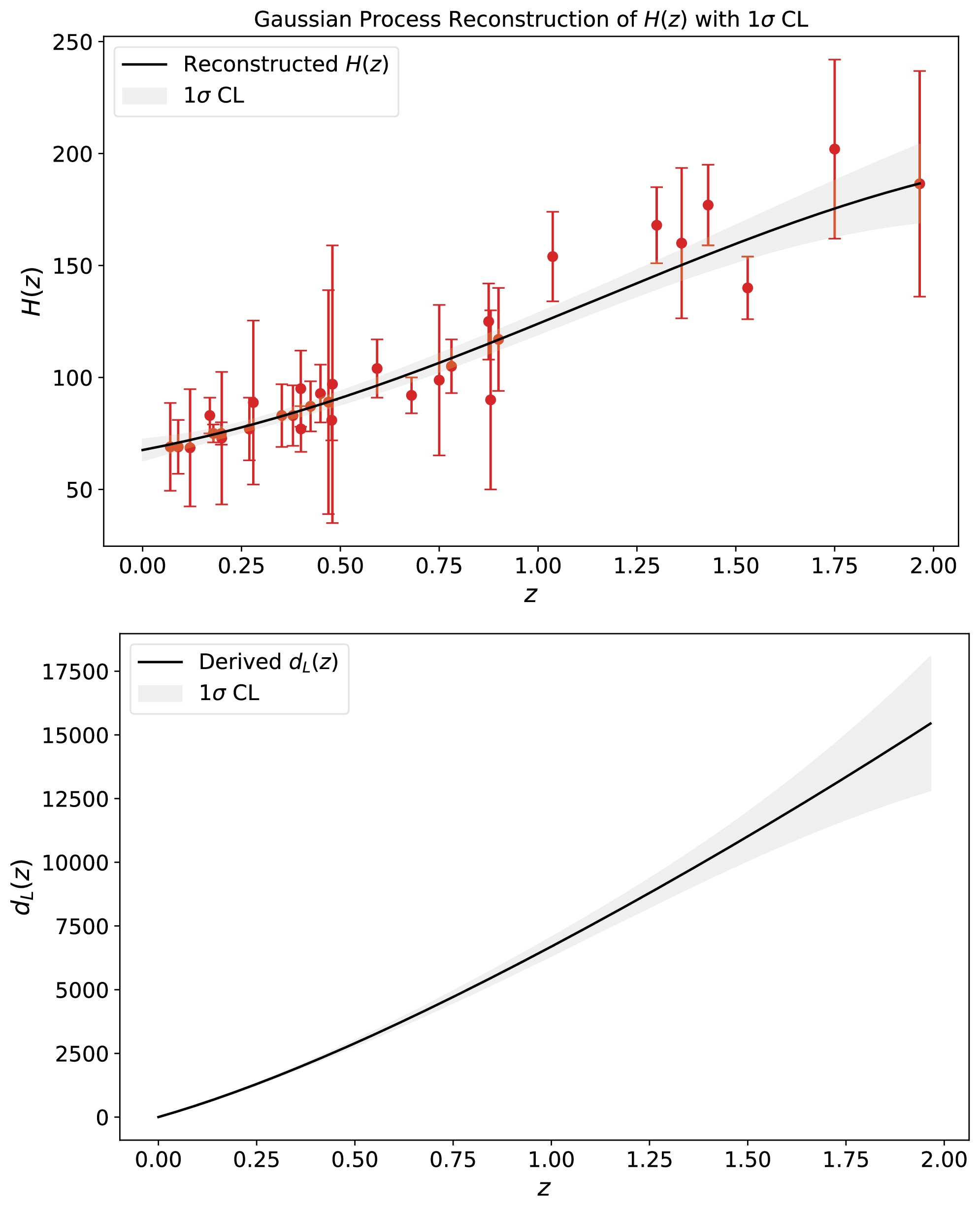

Figure 6.  (color online) Reconstructed $ H(z) $ from 32 Hubble parameter measurements and luminosity distance $ d_L(z) $ derived from this $ H(z) $. The shadows denote 1σ uncertainty.

The cosmological constraints are shown in Fig. 7. For the ΛCDM model, we obtained $ H_0=55.8^{+1.1}_{-1.6} \; {\mathrm{km\, s^{-1}\, Mpc^{-1}}} $ and only a lower bound expressed as $ \Omega_{m0}>0.914 $ using the standard $ L_\mathrm{X} $-$ L_\mathrm{UV} $ relation. In contrast, using the new relation yields effective constraints: $ H_0=70.2\pm3.3 {\mathrm{km\; s^{-1}\, Mpc^{-1}}} $ and $ \Omega_{m0}=0.344^{+0.065}_{-0.093} $. The resulting $ H_0 $ value is consistent with measurements from Planck 2018 ($ H_0=67.4\pm 0.5\; \mathrm{km}\; \mathrm{s}^{-1}\;\mathrm{Mpc}^{-1} $) [53] and from nearby type-Ia supernovae calibrated with Cepheids ($ H_0=73.04\pm 1.04 \mathrm{km}\;\mathrm{s}^{-1}\;\mathrm{Mpc}^{-1} $) [54].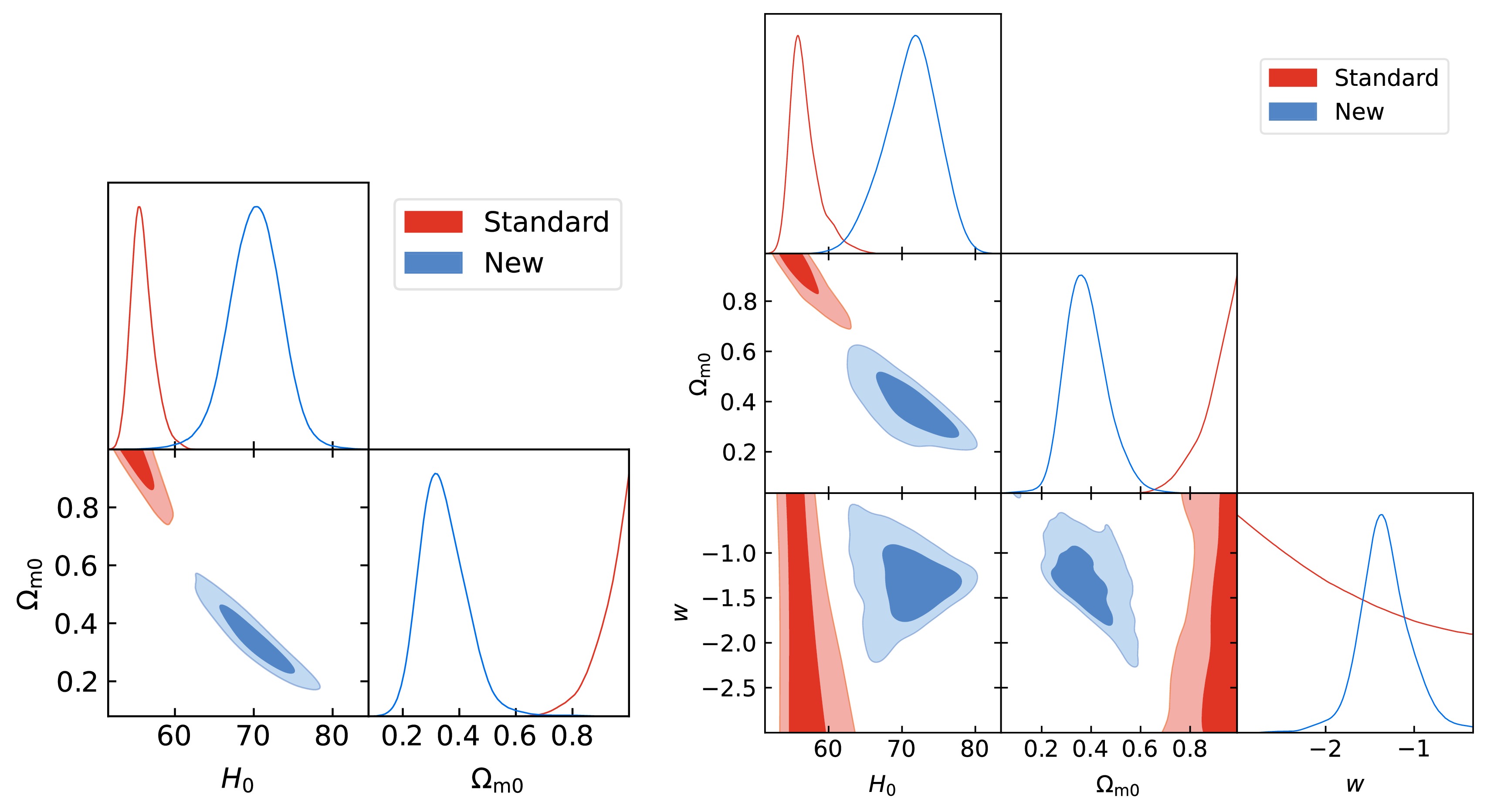

Figure 7.  (color online) Constraints on the ΛCDM and wCDM models from full 2421 quasars standardized with the standard and new $ L_\mathrm{X} $-$ L_\mathrm{UV} $ relations, respectively.

For the wCDM model, quasars with the standard relation provide weak constraints, yielding $H_0=56.7^{+1.1}_{-2.3} {\mathrm{km\; s^{-1}\; Mpc^{-1}}}$, $ \Omega_{m0}>0.883 $, and $ w<-1.45 $. By employing the new relation, we achieved significantly improved constraints: $ H_0=71.2^{+4.0}_{-3.2}\; {\mathrm{km\; s^{-1}\; Mpc^{-1}}} $, $ \Omega_{m0}=0.380^{+0.068}_{-0.095} $, and $ w=-1.33^{+0.25}_{-0.29} $. These results align with those from the Planck 2018 CMB data within 2σ CL [53]. Our findings clearly show that quasars standardized by the proposed relation yield robust and effective cosmological constraints, unlike those standardized by the conventional relation.

Quasars play a crucial role as cosmological probes; constructing accurate luminosity relations for them is essential for their use in cosmology. In this study, we thoroughly tested the redshift variation of the widely used $ L_\mathrm{X} $-$ L_\mathrm{UV} $ relation in quasars. Our analysis reveals a strong linear dependence of the relation coefficients on redshift. Specifically, quasars at higher redshifts favor larger values of β and smaller values of γ compared to those at lower redshifts. These results are consistent with previous findings [37, 38], where quasars were divided into high- and low-redshift subsamples. Importantly, this correlation is not due to the selection effect. For two three-dimensional and redshift-evolving $ L_\mathrm{X} $-$ L_\mathrm{UV} $ relations, we observed that the relation coefficients continue to evolve with redshift. This indicates that the redshift-dependent terms in these evolutionary relations are not sufficient to eliminate the effect of redshift evolution in the coefficients. Finally, we propose a new $ L_\mathrm{X} $-$ L_\mathrm{UV} $ relation that contains four coefficients and found that, in this new relation, the relation coefficients evolve very weakly with redshift. This new relation suggests that the redshift evolution effect can be effectively minimized. Using the Hubble parameter measurements to calibrate the newly proposed relation of quasars, we demonstrate that quasars effectively constrain the ΛCDM and wCDM models. The resulting cosmological constraints are consistent with those derived from Planck CMB observations. Our results indicate that this new $ L_\mathrm{X} $-$ L_\mathrm{UV} $ relation allows quasars to be regarded as more reliable cosmological indicators. The elimination of redshift dependence in the relation could provide a more reliable framework for using quasars in cosmological applications.