Bremsstrahlung emission from nucleon-nucleus reactions in dense medium of compact stars

Light from stars provides key information about them. Stars have nuclei of various masses (for example, see book [1] for the nuclei in the Sun). The convergence in the numeric calculations of the spectra of photons emitted in nuclear processes is obtained while accounting for the space region up to atomic shells. Therefore, it is important to study the nucleus as a system of evolving nucleons in a many-body quantum mechanical problem. This is a basis for studying the emission of photons produced in nuclear reactions in stars. Similar information about photons could be extracted from nuclear collisions at relativistic velocities, and such photons are the subject of this research.

Motivation to study bremsstrahlung photons in nuclear physics can be explained in the following. Bremsstrahlung photons are emitted in reactions and can be measured in experiments. Analysis of the bremss-trahlung spectra during nuclear processes provides additional information about nuclear mechanisms, interactions, etc. Such information obtained from bremss-trahlung analysis can be more deep in comparison with study of the same nuclear reactions without bremss-trahlung analysis. The reason for this is as follows: there are experimental limitations in cross-sectional measurements of nuclear reactions (without measurements of photons); however, one can overcome these limitations through bremsstrahlung measurements and analysis. Some proposals have already been realized in this regard, such as the study of the internal structure of nucleons in nucleon-nucleus scattering at low energies via bremsstrahlung analysis that is proposed as a new type of microscopy of microworld [2]. Based on this, bremsstrahlung analysis of strangeness in hypernuclei was studied [3], deformations of nuclei in α decays were extracted from experimental data [4], information about the dynamics of ternary fission of heavy nuclei was extracted [5−7], the structure and clusters in nuclei in scattering were studied [8, 9], and Δ-resonances in nuclei in proton-nucleus scattering were investigated [10]. Many predictions by such models have been proposed for further experimental study. One attractive idea is to extend the study of bremsstrahlung processes to the conditions of dense media, which can have high-energy collisions in their nuclei. Possible measurements of bremsstrahlung photons can give new uniqual information about the physics of such processes. However, for such investigations, a new bremsstrahlung model must be constructed on a strict quantum mechanical basis (which does not exist yet), taking the properties and mechanisms of nuclear scattering into account.

The study of nuclear forces [12, 13] under extreme conditions in compact stars can widen our understand, and stars are a good laboratory for this [14−16]. This idea is one of the motivations of this research. Many-nucleon unified theories of nucleus and nuclear reactions (see microscopic cluster models based on resonating group method [17−19] and generator coordinate method [20]), shell models, collective models, relativistic mean-field (RMF) theory [21−33], Ab initio calculations theory [34], QCD approaches for systems of nucleons, and quark-meson models [35] have been developed to study nuclei and reactions. In stars, a main focus is to obtain the equation of state (EoS) [36]. Many models have been employed for such a task (for example, see Refs. [37−40] for RMF theories, and see Ref. [36] for Ab initio calculations theory). The Akmal, Pandharipande, Ravenhall (APR) model [41] based on quantum mechanics is one of the most successful (see Refs. [42−45]).

In this paper, we study emission of bremsstrahlung photons from the scattering of neutrons and protons off nuclei under experimental conditions and in compact stars [46−48]. We develop a new bremsstrahlung model for nuclear reactions, where we generalize the quantum mechanical model of the deformed oscillator shells (DOSs) of nuclei [49−52]. We analyze how much the spectra of photons differ between emission from nuclear reactions in conditions on Earth and in the dense medium of stars. As shown in Refs. [53, 54], even for the same full stationary wave functions with the same boundary conditions, there are different nuclear processes (with the same nuclei and energies) in which the difference in cross-sections can be up to 3−4 times. RMF theories cannot explain such a quantum phenomenon, which is important for understanding nuclear processes. Motivated by this, we use quantum mechanics for analysis. It turns out that the DOS model is convenient for such research. ¹

The remainder of this paper is organized as follows. In Sec. II, the emission of bremsstrahlung photons in the scattering of protons and neutrons off nuclei in the dense stellar medium is formulated. In Sec. III, the matrix elements of photon emission are derived for even-even nuclei based on the DOS model. The emission of photons from the nucleon-nucleus scattering for nuclei from ⁴He to ⁵⁶Fe in stars is analyzed in Sec. IV. Conclusions are summarized in Sec. V. Appendixes A and B include some useful analytical formulas for some light nuclei and the derivation of nucleus energy correction due to influence of the stellar medium.

For the first time, we study how the dense medium of a star influences the emission of photons during nuclear reactions. Some calculations have been performed for proton-capture reactions in stars [55, 56]. However, the nuclei in those calculations were studied as stable, without influence from the stellar medium. Now, we will take the deformation of nuclei due to the influence of the stellar medium into account. To be closer to such analysis, we consider the scattering of nucleons on nuclei.

Let us write the Hamiltonian for the scattering of a proton off a nucleus in the stellar medium as

Bremsstrahlung photons emitted in this nuclear process can be described via additional new operator $ \hat{H}_{\gamma} $ as

A concrete form of this operator $ \hat{H}_{\gamma} $ should be defined explicitly. $ V_{\rm star} (|{\bf{r}}_{i} - {\bf{r}}_{j}|) $ will be determined in Sec. III.B.

The emission of bremsstrahlung photons without the influence of stellar medium (i.e., without the last term in Eq. (2)) for the scattering of protons off nuclei on Earth has been studied by many researchers. Here, agreement between theory and existing experimental information has been obtained with the highest precision for this reaction in the frameworks of Refs. [56, 57] (this is data [58] for $ p+^{208}\text{Pb} $ at a proton beam energy of $E_{p}=145$ MeV (see PhD thesis [59] also), data [60] for $ p+^{12}\text{C} $, $ p+^{58}\text{Ni} $, $ p+^{107}\text{Ag} $, $ p+^{197}\text{Au} $ at a proton beam energy of $E_{p}=190$ MeV, and the corresponding calculations in Figs. 5–8 in Refs. [56]). Therefore, we will generalize the bremsstrahlung formalism for these reactions from above-zero up to intermediate energies in stars based on the results of Refs. [56, 57] (see developments in Refs. [2, 3, 55, 61]).

This bremsstrahlung formalism has been tested on the experimental data of bremsstrahlung in α-decay, proton-nucleus scattering, and spontaneous fission [2, 4, 6, 7, 55−57]. It predicts the bremsstrahlung spectra for π-nucleus scattering, radioactivity with proton emission, ternary fission, scattering of α-particles on hypernuclei [3, 5, 57, 61]. At first, proton spin was included in such a formalism in Ref. [57], where scattering of protons off nuclei was studied. However, such a bremsstrahlung was of coherent type, and some experimental bremsstrahlung data were explained in such a way. However, more careful measurements of bremsstrahlung emission in the scattering of protons off nuclei were obtained by TAPS collaborations [60] (we use those data for tests of calculations in the current paper). Those data cannot be described based soley on the coherent bremsstrahlung (there is a plateau in the data not explained in such a way). With this motivation, the previous formalism was improved, where spins of nucleons of the nucleus-target were taken into account. For each nucleon, the scattering proton spin and magnetic moments are used in calculations of the spectra. A new contribution of incoherent emission appeared in the matrix element. That model [56] better describes the experimental data of TAPS for proton-nucleus scattering. It was estimated that incoherent emission is essentially larger than coherent emission. In this paper, we predict ratios between incoherent and coherent bremsstrahlung contributions for different nuclei from ⁴He to ⁵⁶Fe.

We define the cross-section of bremsstrahlung emission for reactions in experiments in the laboratory framework of Ref. [57], where the matrix element of emission is

matrix elements are

coefficients are defined as

and integrals are defined as

Here, $ {\bf{r}} $ is the radius-vector from the center-of-mass of the nucleus to the scattered proton, $ \mu = m_{\rm p}\, m_{A} / (m_{\rm p} + m_{A}) $ is the reduced mass, A is the number of nucleons in the nucleus, $ c_{\rm p} = m_{\rm p}/ (m_{\rm p}+m_{A}) $, $ {\bf{e}}^{(\alpha)} $ are unit vectors of polarization of the photon emitted [$ {\bf{e}}^{(\alpha), *} = {\bf{e}}^{(\alpha)} $], $ {\bf{k}}_{\rm ph} $ is the wave vector of the photon, and $ w_{\rm ph} = k_{\rm ph} c = \bigl| {\bf{k}}_{\rm ph}\bigr|c $, $ E_{\rm ph} = \hbar w_{\rm ph} $ is photon energy. The vectors $ {\bf{e}}^{(\alpha)} $ are perpendicular to $ {\bf{k}}_{\rm ph} $ in Coulomb gauge. We have two independent polarizations $ {\bf{e}}^{(1)} $ and $ {\bf{e}}^{(2)} $ for the photon with impulse $ {\bf{k}}_{\rm ph} $ ($ \alpha=1,2 $). $ \mu_{\rm pn}^{\rm (an)} = \mu_{\rm p}^{\rm (an)} + \mu_{\rm n}^{\rm (an)} $, where $ \mu_{\rm p}^{\rm (an)} $ and $ \mu_{\rm n}^{\rm (an)} $ are anomalous magnetic moments of protons and neutrons, respectively.

The matrix elements $ M_{p}^{(E,\, {\rm dip},0)} $ and $ M_{p}^{(M,\, {\rm dip},0)} $ describe coherent bremsstrahlung emission of photons of electric and magnetic types, and the matrix elements $ M_{\Delta E} $ and $ M_{\Delta M} $ describe incoherent bremsstrahlung emission of photons of electric and magnetic types, respectively. $ M_{P} $ is related to the motion of the full nuclear system, which we neglect in this paper. The effective electric charge and magnetic moment of the system in the dipole approximation (i.e., at $ {\bf{k_{\rm ph}}} {\bf{r}} \to 0 $) are

$ m_{\rm p} $ and $ z_{\rm p} $ are proton mass and charge, and$ m_{A} $ and $ z_{A} $ are nucleus mass and charge, respectively. We introduce the magnetic moment of the nucleus as

where $ \mu_{j}^{\rm (an)} $ is the anomalous magnetic moment of a proton or neutron in the nucleus, $ m_{Aj} $ is the mass of nucleon j in the nucleus, and $ {\boldsymbol{\sigma}} $ is the spin operator.

In this paper, we use the folding approach to describe the scattering of a nucleon in a nucleus. This approach is an approximation of a more complicated and fully microscopic (cluster) formalism describing nuclear reactions with structure on nuclei on the strict basis of quantum mechanics and using nucleon-nucleon interactions in the basis (see App. C for more details). Here, formalisms of the center-of-masses of the nucleus and full nucleon-nucleus system in the scattering are natural parts of the microscopic formalism. Some developments of that approach for reactions with light nuclei are given by us in Refs. [8, 9], where we included the formalism of bremsstrahlung photon emission. In these papers, there are references to other papers with explanations of a more detailed cluster formalism without emission of photons but with analysis of different peculiarities of that approach.

We apply the nuclear model of deformed oscillatoric shells (DOSs; see Appendix A) to describe the nucleus structure, where the Hamiltonian of A nucleons is defined as [49]

The potential energy of two-nucleon nuclear interactions and potential energy of Coulomb forces between protons are defined as (see Eqs. (2.5) and (2.6) in Ref. [52] and Eq. (15) in Ref. [49])

where proton density (for nuclei with an even number of protons) is

Here, summation is performed over all states of configuration, $ H_{n}(x) $ are Hermitian polynomials [we use the definition from Ref. [62], p. 749, (а,6)], a, b, c are oscillator parameters along the x, y, z axes, respectively. Neutron density $ F_{n} (n; {\bf{r}}_{i}, {\bf{r}}_{j}) $ is obtained after a change of proton configuration and numbers of states on the corresponding neutron characteristics.

The kinetic energy of nucleons in the center-of-mass frame is defined as (see Eq. (2.4) in Ref. [52])

The radii of proton and neutron density distributions are defined as [49]

Here, $ a_{\rm p} $, $ b_{\rm p} $, and $ c_{\rm p} $ are oscillator parameters along the x, y, z axes for protons, and $ a_{\rm n} $, $ b_{\rm n} $, $ c_{\rm n} $ for neutrons. We use the approximation $ a_{\rm p} = a_{\rm n} = a $, $ b_{\rm p} = b_{\rm n} = b $, $ c_{\rm p} = c_{\rm n} = c $.

The potential energies for Coulomb and nuclear interactions and kinetic energy are integrated partially analytically for even-even nuclei (see calculations for some light nuclei in Sec. A.3). However, for general analysis of the properties of nuclei in the large region on numbers of protons and neutrons, it is more effective to integrate such energies numerically. It turns out that such an approach allows the influence of a dense stellar medium of a compact star on nuclei to be analyzed easily in this wide region in a unified manner. Table 1 presents the results of calculations of binding energy (per nucleon), oscillating lengths, and radii of proton and neutron density distributions for ground states of even-even nuclei by such an approach.

Nucleus	$ (E_{\rm full}/A) $/MeV	$ E_{\rm nucl} $/MeV	$ E_{\rm Coul} $/MeV	$ E_{\rm kin} $/MeV	a/fm	b/fm	c/fm	$ R_{\rm p} $/fm	$ R_{\rm n} $/fm
4He	−8.462	−125.18	1.11	90.22	1.03	1.03	1.03	1.09	1.09
6He	−2.520	−109.90	0.64	94.14	1.59	1.29	1.29	1.56	1.93
8He	−0.748	−100.92	0.43	94.51	1.50	1.77	1.77	1.93	2.42
10He	−0.091	−98.61	0.43	97.29	1.91	1.91	1.91	2.22	2.77
8Be	−5.549	−207.83	1.29	162.17	1.54	1.15	1.15	1.84	1.84
10Be	−3.496	−204.32	1.29	168.07	1.62	1.46	1.27	2.04	2.11
12Be	−2.475	−203.91	1.23	172.98	1.69	1.55	1.54	2.22	2.33
14Be	−1.785	−213.95	1.07	187.88	1.94	1.59	1.58	2.44	2.97
12C	−5.170	−291.56	1.71	227.80	1.48	1.34	1.34	2.00	2.00
14C	−4.603	−307.63	1.49	241.69	1.52	1.51	1.38	2.13	2.16
16C	−3.672	−314.38	1.41	254.21	1.73	1.55	1.44	2.31	2.73
18C	−2.915	−319.15	1.87	264.79	1.78	1.76	1.49	2.46	3.09
16O	−6.283	−407.27	2.10	304.64	1.41	1.41	1.41	2.08	2.08
18O	−5.255	−417.09	2.20	320.30	1.60	1.44	1.44	2.21	2.57
20Ne	−5.966	−497.98	2.95	375.69	1.66	1.39	1.39	2.59	2.59
22Ne	−5.118	−502.28	3.23	386.44	1.68	1.55	1.42	2.68	2.86
24Mg	−5.587	−575.07	4.82	436.15	1.62	1.62	1.39	2.85	2.85
26Mg	−4.923	−580.27	4.87	447.38	1.64	1.63	1.53	2.93	3.03
28Si	−5.312	−649.71	5.83	495.12	1.60	1.60	1.60	3.03	3.03
30Si	−5.301	−687.11	5.94	522.11	1.64	1.63	1.58	3.06	3.06
32S	−5.898	−771.79	6.21	576.82	1.63	1.62	1.54	3.03	3.03
34S	−5.970	−818.32	6.05	609.28	1.65	1.62	1.56	3.05	3.04
36Ar	−6.545	−899.80	7.03	657.13	1.65	1.59	1.57	3.03	3.03
38Ar	−6.687	−949.80	6.93	688.73	1.64	1.61	1.60	3.05	3.04
40Ar	−6.218	−965.37	6.84	709.82	1.66	1.63	1.65	3.11	3.14
40Ca	−7.285	−1044.28	7.56	745.29	1.60	1.60	1.60	3.01	3.01
42Ca	−6.963	−1072.27	7.82	772.45	1.62	1.62	1.62	3.06	3.09
44Ca	−6.665	−1097.52	7.93	796.32	1.67	1.64	1.62	3.11	3.25
50Cr	−6.788	−1260.28	8.43	912.41	1.73	1.65	1.62	3.30	3.39
52Cr	−6.629	−1293.79	8.53	940.84	1.73	1.69	1.64	3.33	3.49
54Fe	−6.830	−1364.49	8.93	986.71	1.74	1.66	1.64	3.42	3.49
56Fe	−6.788	−1405.45	9.43	1015.87	1.75	1.70	1.64	3.45	3.58
58Fe	−6.662	−1440.90	9.92	1044.59	1.75	1.71	1.67	3.47	3.65

Table 1.  Energies, oscillating parameters, and radii of proton and neutron density distributions for ground states of even-even nuclei from ⁴He to ⁵⁶Fe, calculated by Eqs. (10), (11), (13), and (14). We also include contributions from the potential energy of nuclear two-nucleon interactions and the Coulomb and kinetic terms. One can see that the role of Coulomb interactions in the calculations of binding energy is small.

Note that this formulation of the Hamiltonian of the DOS model also includes a term for correction of the nucleus center-of-mass (see last term in Eq. (13)). Different variants of the center-of-mass correction were analyzed by Steshenko and Filippov in that model, and finally they provided the most suitable formulation of hamiltonian, which we use now. We also calculated binding energies for different nuclei, starting from light ⁴He. We found that the calculated binding energies for light nuclei are sufficiently close to the experimental data. We found that the DOS explains the existence of bound states of isotopes of light nuclei and the non-existence of bound states of further isotopes of these nuclei after increasing the number of neutrons in a unified manner. The model also explained that only ⁴He is spherical, while other isotopes of Helium and other nuclei have deformations. The model calculates deformations for those nuclei. Refs. [49, 50] compared calculated deformations with available experimental information for light nuclei and found good agreement. All these DOS model results (see Table 1) are based on the chosen form of kinetic term with fixed correction of the nucleus center-of-mass.

Note that with nucleon-nucleon potentials based on meson exchange, which are used in calculations of binding energies of nuclei, some electromagnetic interactions (and parametrizations) are different: Argonne potential [63], CD-Bonn potential [64], Nijmegen potential [65], Reid93 potential [65], and Paris potential [66]. Coulomb interactions are electromagnetic interactions with magnetic moments of protons and neutrons. One approach [67] provided an accurate study of Coulomb interactions on the basis of Hartree-Fock calculations within Bardeen-Cooper-Schrieffer approximation using seniority force. Our bremsstrahlung formalism includes anomalous magnetic moments of protons and neutrons of nuclei and of scattered protons or neutrons. Matrix elements of emission can be calculated based on the wave functions of the DOS model. Therefore, the bremsstrahlung formalism calculates the spectra of photons, and these spectra are dependent on magnetic moments of protons and neutrons of the nuclear system. The bremsstrahlung approach allows the magnetic moments of nucleons in nuclear reactions to be studied.

The role of nucleons magnetic moments in producing incoherent bremsstrahlung is more essential than in calculations of binding energies. We estimate the following ratios between incoherent and coherent contributions to the full spectrum: $ \dfrac{\sigma_{\rm incoh} (^{4}\text{He})}{\sigma_{\rm coh} (^{4}\text{He})} = 3.2340 $, $\dfrac{\sigma_{\rm incoh} (^{8}\text{Be})}{\sigma_{\rm coh} (^{8}\text{Be})} = 58.629$, $ \dfrac{\sigma_{\rm incoh} (^{12}\text{C})}{\sigma_{\rm coh} (^{12}\text{C})} = 299.20 $, $ \dfrac{\sigma_{\rm incoh} (^{16}\text{O})}{\sigma_{\rm coh} (^{16}\text{O})} = 947.7 $, $\dfrac{\sigma_{\rm incoh} (^{24}\text{Mg})}{\sigma_{\rm coh} (^{24}\text{Mg})} = 4817.7$, $\dfrac{\sigma_{\rm incoh} (^{40}\text{Ca})}{\sigma_{\rm coh} (^{40}\text{Ca})} = 3.720 \times 10^{4}$, $\dfrac{\sigma_{\rm incoh} (^{56}\text{Fe})}{\sigma_{\rm coh} (^{56}\text{Fe})} = 1.7592 \times 10^{5}$.

A neutron star radius is approximately 10–14 km. The radii of typical white dwarfs are approximately 5000 km [46], while the radius of their nuclei is up to approximately 10–15 fm. The difference between the sizes of nuclei and space regions of compact stars is huge. Thus, under a proper approximation, one can study the influence of the medium of a star on nucleons of a nucleus in the homogeneous approximation (near this nucleus), while the influence of inhomogeneous effects can be estimated as corrections. The evolution of particles in the homogeneous external field is a standard topic of quantum mechanics (for example, see book [62], p. 103–105), where the linear force acting on a particle corresponds to such an approximation. One folding approach describes the structure of nuclei via integration of the density distribution of nuclear matter. This approach is successful in describing experimental data of nuclear scattering, fusion, and spontaneous and ternary fission with very good accuracy.

Let us write the Hamiltonian of a nucleus with influence of the stellar medium on nucleons as

where $ T_{\rm full} $ is defined in Eq. (13). In the first approximation, we shall assume that the influence of the stellar medium on nucleons of the studied nucleus is homogeneous. The force $ {\bf{F}} $ of such an influence depends on distance R between center of the star and center of mass of the studied nucleus. The potential of such an influence depends on relative distances between nucleons of the studied nucleus. ² Following quantum mechanics (see Ref. [62], p. 100–102, for details), we define it as ³

The correction $ \Delta E_{\rm star} $ to the full energy of the nucleus due to inclusion of the influence of the star on nucleons of the nucleus can be defined as

Such a matrix element is calculated in B. For even-even nuclei (at $ Z=N $), we obtain

In particular, for ⁴He, we have (see Eq. (69) at $ a=b=c $)

where $ F_{P} (R) = |{\bf{F}}_{P} (R)| $. In a general case, we obtain

Thus, we have the following picture of the influence of stellar medium on the studied nucleus. Forces of the stellar medium press on nucleons of the nucleus. The deeper this nucleus is located in the star, the stronger such forces press on the nucleus. However, binding energy (which is negative for nucleus in the external layer of star) is increased at deeper locations of this nucleus in the star. Starting from some critical distance from the nucleus to the center of the star, the binding energy becomes positive. Thus, the full energy of individual nucleons of the studied nucleus is already larger than the mass of this nucleus, i.e., we obtain an unbound system of nucleons, and the nucleus is disintegrated on nucleons. It could be interesting to estimate if such a phenomenon appears in white dwarfs and neutron stars. The kinetic energy is increased at deeper locations of the nucleus in a star. At decreasing distance from the studied nucleus to the center of the star, the change of kinetic energy is unlimited, while the change of nuclear energy is limited. Thus, the ratio between kinetic energy of nucleonsand nuclear energy of the nucleus is changes.

For estimations of bremsstrahlung emission for nuclear reactions in a stellar medium, we apply perturbation theory. We formulate the influence of the stellar medium on emission as

From here, we find that the matrix element of emission in a star as

Following perturbation theory, the first correction is determined based on two unperturbed wave functions, i.e., we take wave functions as in the matrix element (3):

where

Here, $ \varphi_{\rm p-nucl} ({\bf{r}}, k_{f}) $ is the wave function of protons scattering off the nucleus (energy has continuous spectrum, as emitted photons take some energy of the proton-nucleus system), and $ \varphi_{0}^{2} ({\bf{r}}) $ is the wave function of the nucleus (energy has only discrete levels, nucleons are only in bound states). We renormalize the wave function of proton scattering off the nucleus ⁴. For ⁴He, we have

Substituting Eq. (26) into (24) for ⁴He (at $ a=b=c $), we obtain

The wave function $ \varphi_{\rm p-nucl} $ of relative motion between a proton and center-of-mass of the nucleus is calculated numerically in terms of the proton-nucleus potential as $ V (r) = v_{c}(r) + v_{N}(r) + v_{\rm so}(r) + v_{l} (r) $, where $ v_{c}(r) $, $ v_{N}(r) $, $ v_{\rm so}(r) $, and $ v_{l} (r) $ are Coulomb, nuclear, spin-orbital, and centrifugal terms with parameters in Eqs. (46)–(47) in Ref. [56]. Note that such calculations of the wave function parameters of proton-nucleus potential are varied based on the folding potential (with tests). This gives faster calculations of the final cross-sections of bremsstrahlung with sufficiently good approximation and stability.

EOSs have been obtained by many authors. These data are presented in the form of tables containing a grid of calculated values of matter density, baryon (number) density, and pressure. Useful analytical representations were derived by Haensel and Potekhin for two EOSs for not-rotating and rotating neutron-star matter [68]: FPS and SLy (see Eqs. (14), (17) in that paper). These results allow those EOSs to be applied to other problems in a fast manner. Thus, we use that result to start our own calculations (and for testing) in terms of the density of stellar matter.

However, to obtain corrections to binding energies of nuclei in the stellar medium, we need to reproduce EOSs in compact stars. One object where a polytropic model has been successfully applied is a white dwarf (see Ref. [15], p. 364–370; Ref. [16], p. 213–233, p. 475–496). According to Ref. [14] (see Fig. 2.2 in that book, p. 33; also see Fig. 103 in Ref. [15], p. 365), the density in the center of such a star is $10^{+5} \;\,{\rm g/}\, {\rm cm}^{3}$ – $1.4 \times 10^{+9}\,\; {\rm g/}\, {\rm cm}^{3}$. Solving the Lane-Emden equation at polytropic index $ n=3 $ by the finite-difference method, we obtain radii for white dwarfs in region of 3011.28 (at $\rho_{\rm cr} = 1.4 \cdot 10^{9}\, \;{\rm g/}\, {\rm cm}^{3}$) to 72 576.27 km (at $\rho_{\rm cr} = 10^{5}\,\; {\rm g/}\, {\rm cm}^{3}$). We perform analysis for such a star.

Let us estimate the force acting on the studied nucleus under the influence of stellar medium. Pressure is force applied perpendicular to the surface of an object per unit area over which that force is distributed. Therefore, the pressure acting on a selected layer in the medium can be represented as force acting on a unit area of this layer. The full force acting on such a layer can be found as the pressure multiplied by the full area of this layer. Thus, the force acting on a nucleus with surface $ S_{\rm nucl} $ in a stellar medium can be determined as pressure multiplied by the surface area of this nucleus as

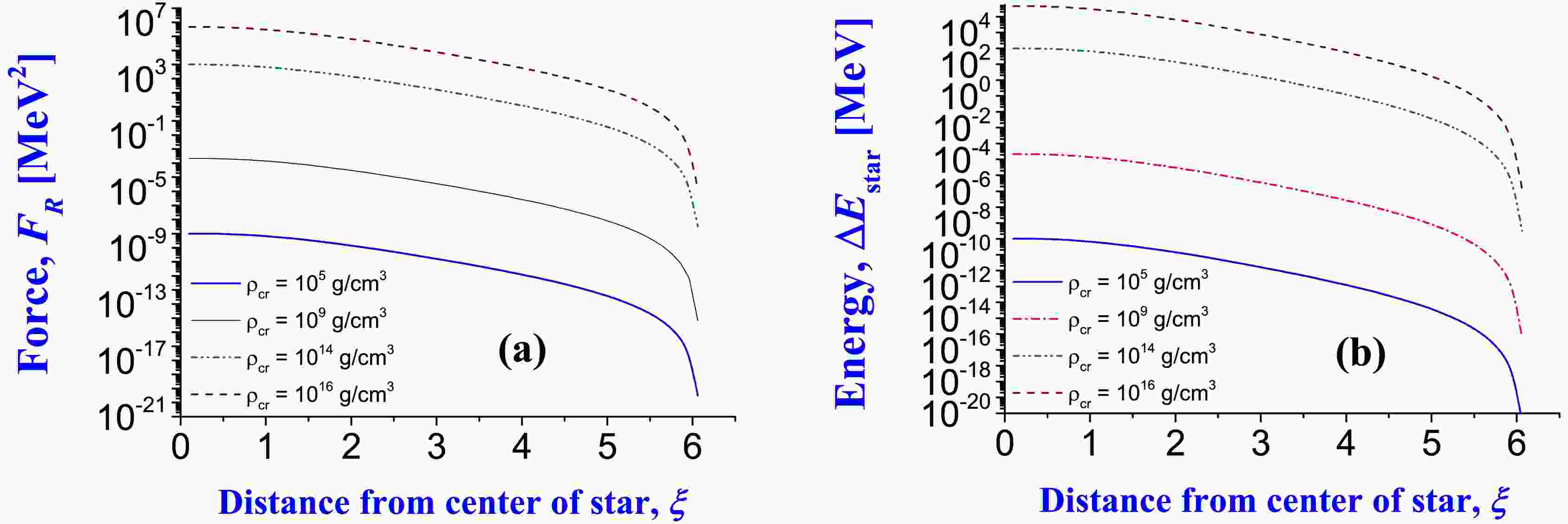
By good approximation, the nucleus can be studied as spherical with $ S_{\rm nucl} = 4\pi\, R_{\rm nucl}^{2} $, $ R_{\rm nucl} = a \cdot A^{1/3} $. The force acting on a ⁴He nucleus in a star is shown in Fig. 1 (a) ⁵.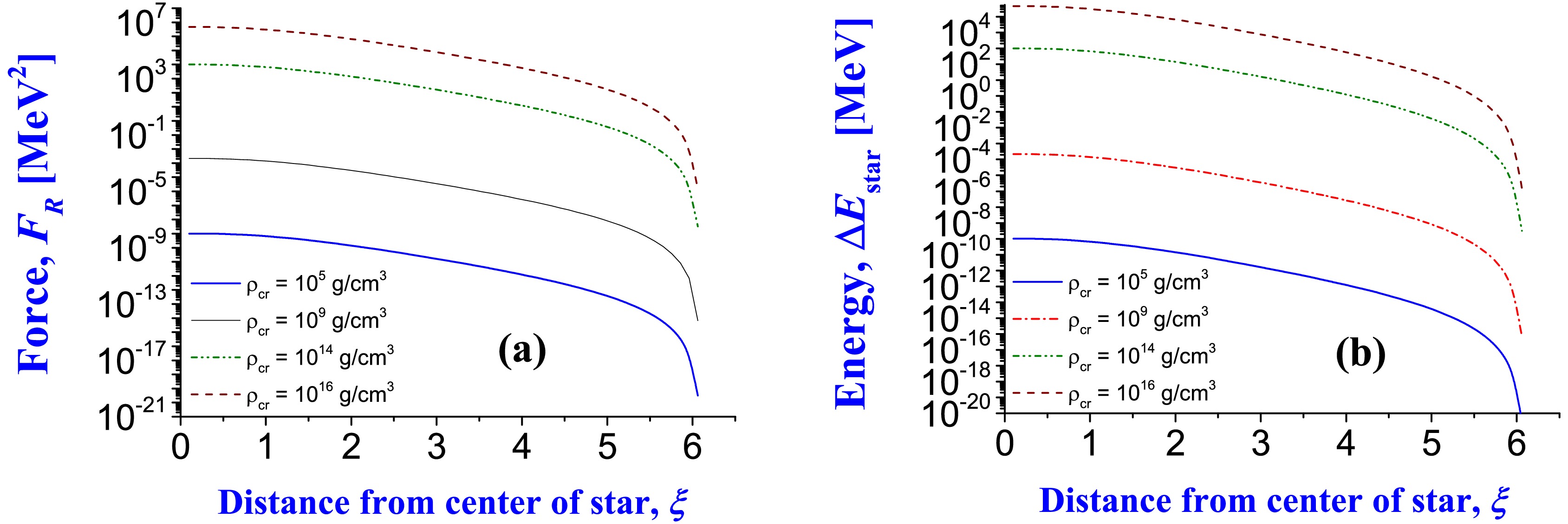

Figure 1.  (color online) Panel (a): Force $ F_{R} $ acting on nucleons of ⁴He nucleus depending on its renormalized distance ξ to the center of the star (at polytropic index $ n=3 $). Force is defined in Eq. (28), and the oscillator parameter $ a=1.05 $ fm is fixed for estimations, which is close to the minimum full energy of ⁴He under natural conditions on Earth]. Panel (b): Correction $ \Delta E $ to the ⁴He nucleus energy due to the influence of stellar medium in terms of distance to the center of the star (at $ n=3 $), Correction of energy $ \Delta E $ is defined in Eq. (20).

Calculated corrections to the full energy of the ⁴He nucleus from such an influence are presented in Fig. 1 (b). One can see that in white dwarfs and the inner and external crusts of neutron stars (densities of $10^{5}\, {\rm g/}\, {\rm cm}^{3}$ – $1.4 \cdot 10^{9}\,\; {\rm g/}\, {\rm cm}^{3}$), nuclei are not disintegrated. However, this phenomenon typically occurs at higher densities, starting from some critical distances from the center of stars (see upper brown dashed line (at $\rho_{\rm cr} = 10^{16}\,\; {\rm g/}\, {\rm cm}^{3}$) and green dash-double dotted line (at $\rho_{\rm cr} = 10^{14}\,\; {\rm g/}\, {\rm cm}^{3}$) in the figure). This case corresponds to densities of the core of neutron stars.

We shall analyze the possibility of the nucleus to disintegrate on individual nucleons in the neutron star ⁶. Different types of energy for a ⁴He nucleus are shown in Fig. 2. One can see that the full energy of the nucleus can already be positive after taking the energy correction shown in Fig. 1 (b) into account. This means that nucleons do not form a bound system, i.e., the nucleus is disintegrated. The oscillator length a corresponding to the minimum of the full energy of the system of nucleons is decreased in comparison with its value for a nucleus in vacuum. Thus, the relative distances between nucleons of ⁴He are decreased. This is explained by the influence of pressure of the stellar medium on nucleons. We obtain similar tendencies for other isotopes of He and Be.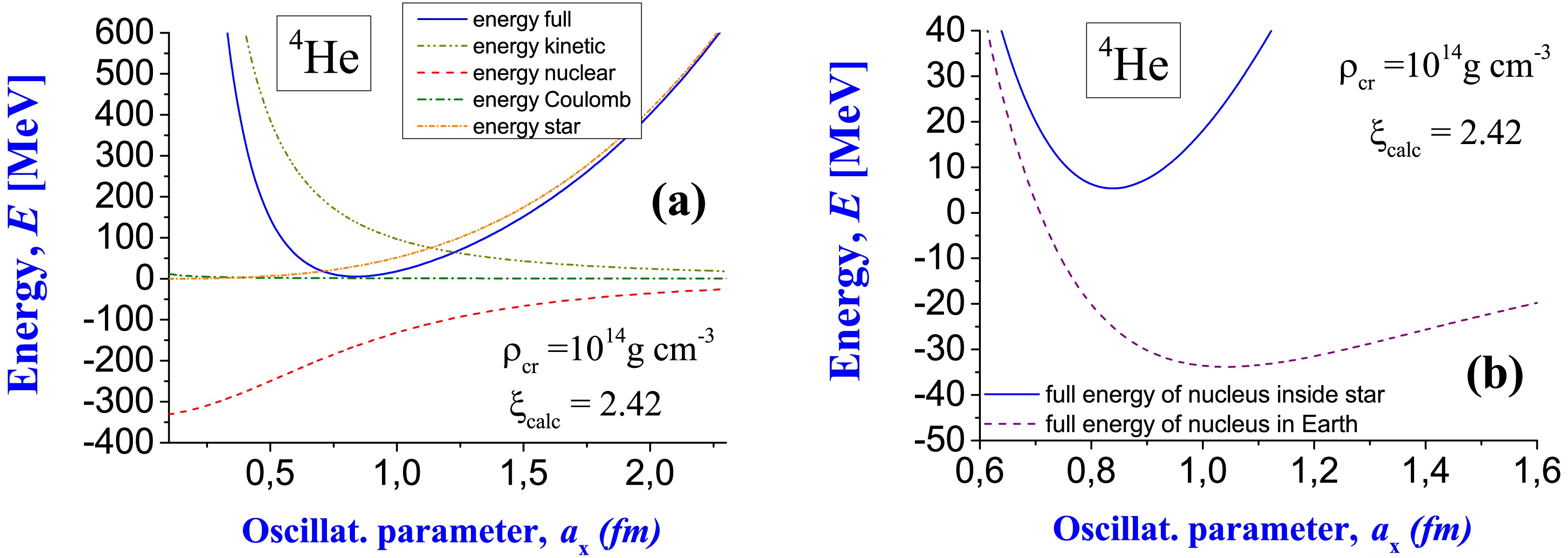

Figure 2.  (color online) Panel (a): Energy of⁴He nuclear system inside a star at distance $ \xi=2.42 $ from the center of the star with a density at the center of $\rho_{\rm cr} = 10^{14}\; {\rm g/}\, {\rm cm}^{3}$ (at $ n=3 $). At the minimum of the full energy of nucleus, we obtain $ a = 0.8374 $ fm, $ E_{\rm full} = 5.038 $ MeV, $ E_{\rm full\, per\, nucl} = 1.327 $ MeV, $ E_{\rm kin} = 138.096 $ MeV, $ E_{\rm Coul} = 1.363 $ MeV, $ E_{\rm nucl} = -164.492 $ MeV, $ E_{\rm star} = 30.313 $ MeV. Panel (b): Full energy of nucleus inside star in comparison with full energy of this nucleus on Earth.

In Fig. 3, we show the energies of nuclear systems of ⁸Be, ¹²C, ¹⁶O, ²⁴Mg, and ⁴⁰Ca, ⁵⁶Fe. The location of disintegration of a nucleus inside the star is presented in Fig. 4.

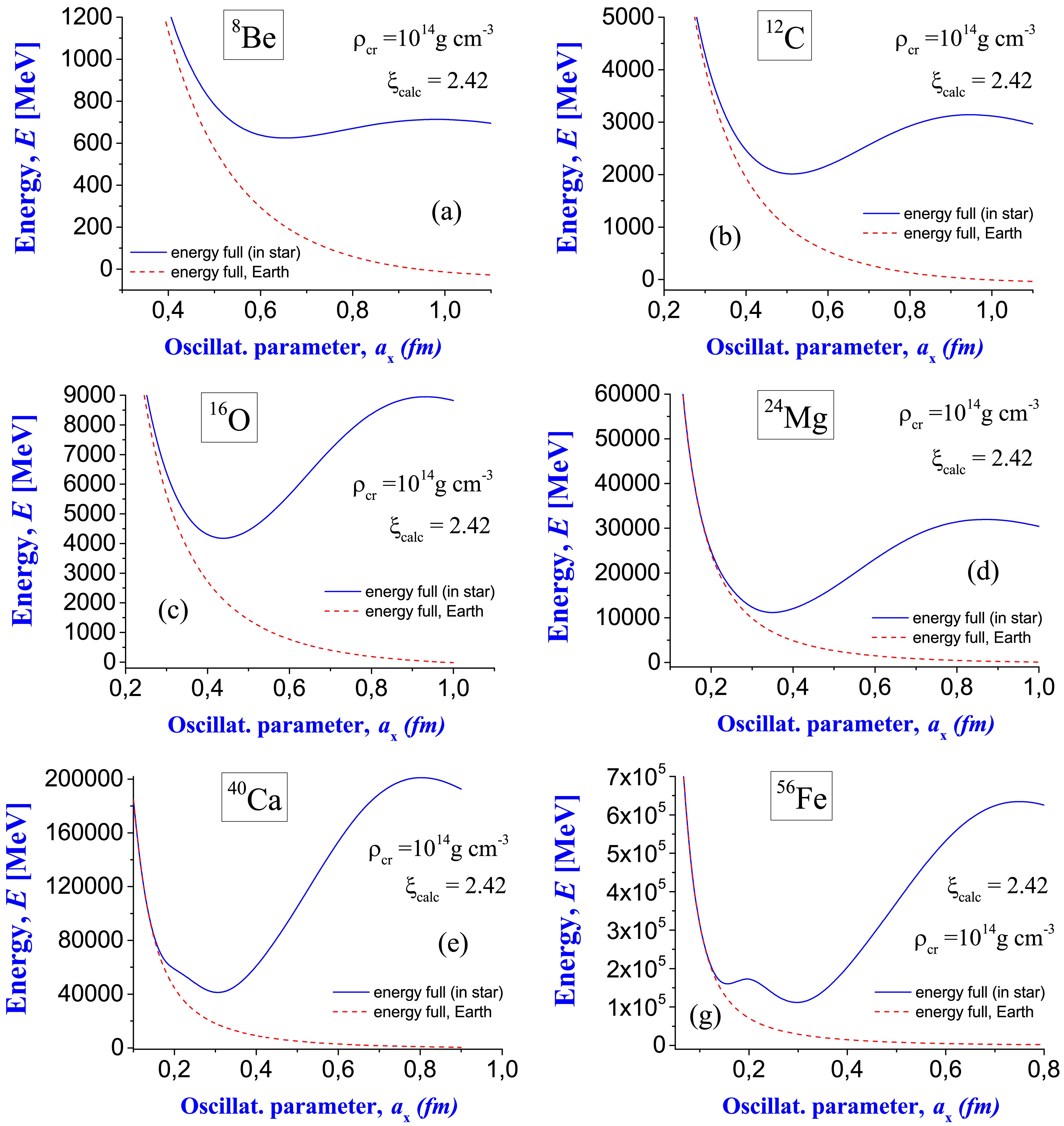
Figure 3.  (color online) Full energy of "nuclei" ⁸Be (a), ¹²C (b), ¹⁶O (c), ²⁴Mg (d), ⁴⁰Ca (e), and ⁵⁶Fe (g) inside dense stellar medium (blue solid lines) in comparison with full energy of these nuclei on Earth (red dashed lines). Here, we use the same position as in Fig. 2 (distance $ \xi=2.42 $ from center of star, density at center $\rho_{\rm cr} = 10^{14}\; {\rm g/}\, {\rm cm}^{3}$). At the minimum of the full energy of ⁸Be, we obtain $ a = 0.64 $ fm, $ E_{\rm full} = 623.90 $ MeV, $ E_{\rm full\, per\, nucl} = 77.98 $ MeV, $ E_{\rm kin} = 638.77 $ MeV, $ E_{\rm nucl} = -431.47 $ MeV, $ E_{\rm star} = 415.31 $ MeV. At the minimum of the full energy of ¹²C, we obtain $ a = 0.51 $ fm, $ E_{\rm full} = 2004.93 $ MeV, $ E_{\rm full\, per\, nucl} = 167.0 $ MeV, $ E_{\rm kin} = 1694.04 $ MeV, $ E_{\rm nucl} = -757.27 $ MeV, $ E_{\rm star} = 1066.45 $ MeV. At the minimum of the full energy of ¹⁶O, we obtain $ a = 0.43 $ fm, $ E_{\rm full} = 4172.6 $ MeV, $ E_{\rm full\, per\, nucl} = 260.7 $ MeV, $ E_{\rm kin} = 3308.0 $ MeV, $ E_{\rm nucl} = -1090.6 $ MeV, $ E_{\rm star} = 1953.2 $ MeV. At the minimum of the full energy of ²⁴Mg, we obtain $ a = 0.34 $ fm, $ E_{\rm full} = 11116 $ MeV, $ E_{\rm full\, per\, nucl} = 463.2 $ MeV, $ E_{\rm kin} = 8672 $ MeV, $ E_{\rm nucl} = -1748 $ MeV, $ E_{\rm star} = 4189 $ MeV. At the minimum of the full energy of ⁴⁰Ca, we obtain $ a = 0.31 $ fm, $ E_{\rm full} = 41130 $ MeV, $ E_{\rm full\, per\, nucl} = 1028.2 $ MeV, $ E_{\rm kin} = 19536 $ MeV, $ E_{\rm nucl} = -2999 $ MeV, $ E_{\rm star} = 24585 $ MeV, $ R_{\rm p} = R_{\rm n} = 0.58 $ fm. At the minimum of the full energy of ⁵⁶Fe, we obtain $ a = 0.28 $ fm, $ E_{\rm full} = 110406 $ MeV, $ E_{\rm full\, per\, nucl} = 1971.5 $ MeV, $ E_{\rm kin} = 363000 $ MeV, $ E_{\rm nucl} = -4068 $ MeV, $ E_{\rm star} = 78164 $ MeV, $ R_{\rm p} = 0.57 $ fm, $ R_{\rm n} = 0.59 $ fm.

Figure 4.  (color online) Critical distance ξ from center of star depending on its density at the center, where disintegration of the ⁴He nucleus on nucleons occurs.

A polytropic model based on the solution of the Lane-Emden equation is inaccurate when describing neutron stars, where the effects of gravity described by general relativity are important. Therefore, for analysis of the bremsstrahlung processes inside neutron stars, we solve equation of Oppenheimer and Volkoff (see Ref. [14], p. 34–36), where non-polytropic dependence of pressure on density is used for relativistic neutrons (see Ref. [46], p. 23–29). The difference between these two approaches for densities at the center of the star in the region of $\rho_{\rm cr} = 10^{14}\, {\rm g/}\, {\rm cm}^{3}$ – $10^{16}\, {\rm g/}\, {\rm cm}^{3}$ is presented in Fig. 5.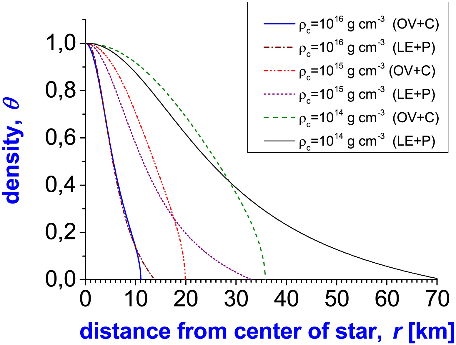

Figure 5.  (color online) Dimensionless density θ inside star based on distance r from center of star, calculated by thr Oppenheimer–Volkoff equation with Chandrasekar (non-polytropic) EOS (OV+C) and by Lane-Emdan equation with polytropic EOS at $ n=3 $ (LE+P). Parameters of calculations: Chandrasekar EOS is defined by Eqs. (2.3.5)–(2.3.6) in Ref. [46] for relativistic neutrons at $ \mu_{e}=1 $ (see p. 25–26 in that book), dimensionless density is defined based on condition $ \rho (r) = \rho_{\rm c} \cdot \theta^{n=3} $ for simplicity of comparison between two approaches. For OV+C, we obtain the following: mass $ M=1.575\; M_{\rm sun} $ and radius $ R=36.00 $ km for star with density at center $ \rho_{\rm cr} = 10^{14}\, {\rm g}\, {\rm cm}^{-3} $; mass $ M=2.276\; M_{\rm sun} $ and radius $ R=19.95 $ km for star with density at center $ \rho_{\rm cr} = 10^{15}\, {\rm g}\, {\rm cm}^{-3} $; and mass $ M=1.655\; M_{\rm sun} $ and radius $ R=11.07 $ km for star with density at center $ \rho_{\rm cr} = 10^{16}\, {\rm g}\, {\rm cm}^{-3} $ ($ M_{\rm sun} $ is mass of the Sun).

Inverse beta decay is important when studying the structure of neutron stars; the simplest EOS taking into account these processes was proposed by Harrison and Wheeler. Such an EOS also provides information about the most probable nuclei based on stellar density. Such estimations are shown in Fig. 6.

Figure 6.  (color online) Distribution of nuclei with mass numbers A (a) and charge numbers Z (b) according to radius for a star with density at the center of $ 10^{14}\, {\rm g}\, {\rm cm}^{-3} $. Here, the Harrison–Wheeler EOS is used in the calculations (we take EOS parameters from Ref. [46], see p. 42–48). This allows to take into account processes of inverse beta decay for higher densities and provide information about the chemical composition inside the star. The finite-difference method is used to solve the Oppenheimer-Volkoff equation for this star). We obtain radius $ R=52.859 $ km and mass of star $ M=0.91072\; M_{sun} $ for such a model.

One can conclude that nuclei can co-exist with neutrons inside a sufficiently long layer in a dense star with density at the center of $10^{14}\, {\rm g/}\, {\rm cm}^{3}$. Although this gives restrictions when considering possible emission of bremsstrahlung photons from different nuclei, we aim to provide a full picture that is useful for a general understanding of the emission of photons from nuclear scattering.

We start calculations of spectra from a case when experimental data are known and agreement between theory and experimental data was obtained with the highest accuracy. This is a case of bremsstrahlung in the scattering of protons of nuclei $ p + $¹⁹⁷Au at a proton beam energy of 190 MeV, where experimental bremsstrahlung data [60] were obtained. In the framework of new formalism described above, we reconstruct the spectra with inclusion of incoherent bremsstrahlung emission (for conditions of measurements).

The important role of incoherent bremsstrahlung emission in the proton-nucleus scattering can be seen from simple calculations. One can use only the largest coherent and incoherent terms at $ l_{i}=0 $, $ l_{f}=1 $, $ l_{\rm ph}=1 $, i.e., we define the coherent term $ M_{\rm coh} $ based on the term $ M_{p}^{(E,\, {\rm dip})} $ and incoherent term $ M_{\rm incoh} $ based on the term $ M_{\Delta M} $ in the calculation of the full matrix element as (see Ref. [10, 56] and references therein for details)

where $ M_{p}^{(E,\, {\rm dip},0)} $ and $ M_{\Delta M} $ are calculated by Eq. (4). Such calculations in comparison with experimental data are presented in Fig. 7 (a). ⁷ One can see that the full spectrum with both coherent and incoherent contributions included (blue solid line in this figure) essentially better describes the experimental data than just the coherent bremsstrahlung (purple dash-dotted line). This essential difference between these two spectra confirms the large role of incoherent emission in the full bremsstrahlung. A main conclusion from this analysis is that incoherent processes are essentially more intensive than coherent processes, and this difference increases with increasing energy of the emitted photon. From this analysis, it is easy to extract the normalization factor, which can be used for other calculations of bremsstrahlung in cases where there is no experimental information about bremsstrahlung.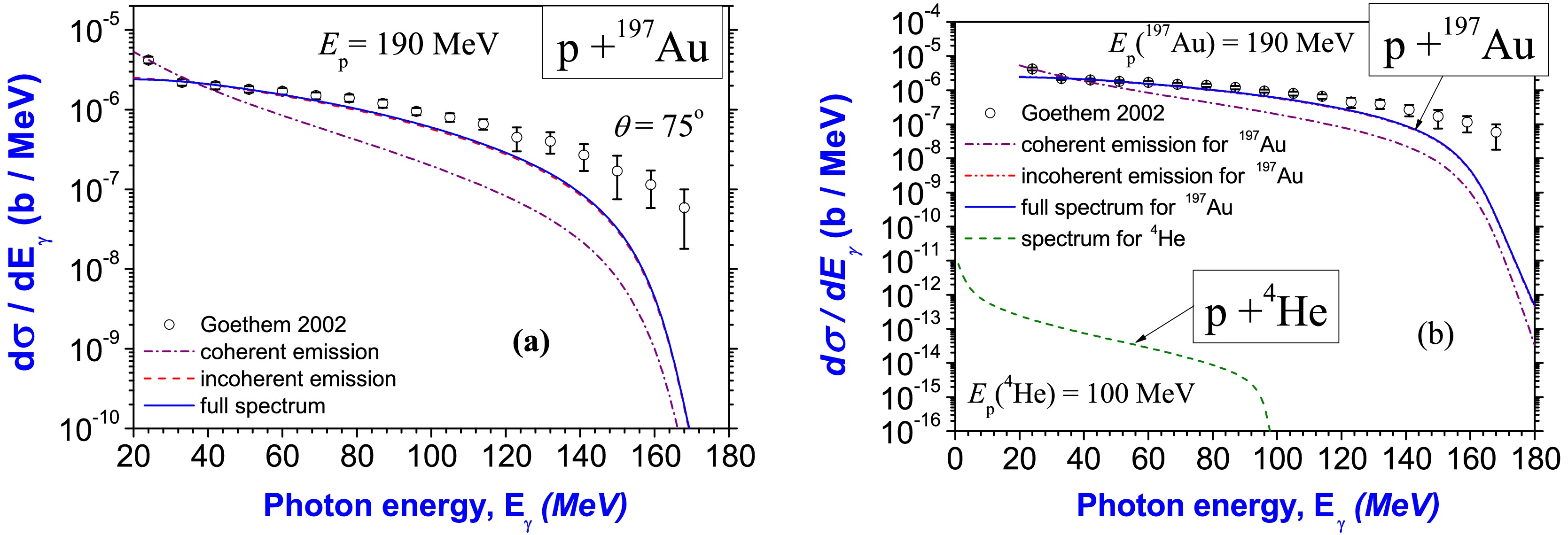

Figure 7.  (color online) Panel (a): Calculated bremsstrahlung spectra in the scattering of protons off ¹⁹⁷Au nuclei at a proton beam energy of $ E_{\rm p}=190 $ MeV in comparison with experimental data [60]. Matrix elements are defined in Eqs. (1)– (3), $ Z_{A} (k_{\rm ph})\simeq Z_{A} $ is electric charge of the nucleus, and we normalize each calculation of the second point of experimental data. Here, open circles are experimental data obtained by TAPs collaboration with high precision [60], the blue solid line is the full spectrum (with coherent and incoherent terms), the purple dash-dotted line is the coherent contribution, the red dashed line is the incoherent contribution. All spectra are renormalized on one point of experimental data. One can see that the full spectrum with inclusion of coherent and incoherent contributions is essentially in better agreement with experimental data than only coherent bremsstrahlung. This result confirms the important role of incoherent emission in bremsstrahlung during the scattering of protons off heavy nuclei (inside such an energy region). One can also see that the role of incoherent processes is increased at increasing photon energy. Panel (b): Calculated bremsstrahlung spectra for the scattering of protons off ⁴He at proton beam energy of $ E_{\rm p}=100 $ MeV in comparison with the calculated spectra and experimental data [60] for the scattering of protons off ¹⁹⁷Au at $ E_{\rm p}=190 $ MeV.

It is also useful to understand the difference between bremsstrahlung emission for heavy and light nuclei under similar conditions. Such calculations (under conditions of experimental laboratory on Earth) are presented in Fig. 7 (b) with comparison between the spectrum for ¹⁹⁷Au at $ E_{\rm p}=190 $ MeV [given in Fig. 7 (a)] and spectrum for ⁴He at $ E_{\rm p}=100 $ MeV. One can see that the difference between the spectra is very large. In particular, more heavy nuclei and larger proton beam energies produce essentially more intensive emission of bremsstrahlung photons. We obtained a similar conclusion in a previous study of bremsstrahlung emission in the fission of nuclei [6, 7] (when we studied separation of parent nucleus ²⁵²Cf on two heavy fragments of similar masses with emission of photons), comparing that with bremsstrahlung in the α decay of nuclei (see Refs. [4, 55] and references therein).

As a next step, we estimate bremsstrahlung in the stellar medium. Here, there are many new questions that have never been studied. As a demonstration, we consider how spectra are changed under the influence of stellar medium. The simplest analysis is obtained from calculations of spectra for ⁴He. We use the normalization factor extracted from the previous study for $ p + $¹⁹⁷Au at 190 MeV, with existing experimental data (see Fig. 7 (a)). New calculations for $ p + $ ⁴He in a dense stellar medium are shown in Fig. 8 (b). We conclude the following: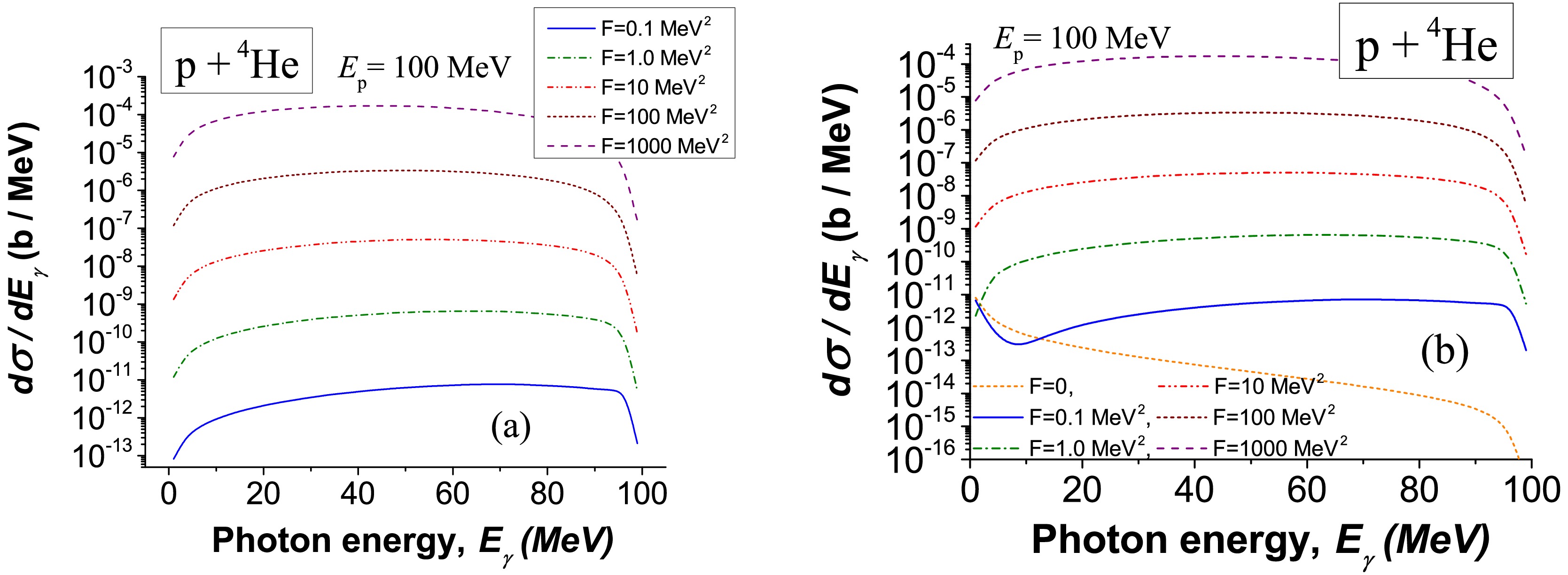

Figure 8.  (color online) Bremsstrahlung emission of photons in scattering of protons off ⁴He nuclei inside star at proton energy of $ E_{\rm p}=100 $ MeV at polytropic index $ n=3 $. We calculate the spectrum based on the leading matrix element $ M_{p}^{(E,\, {\rm dip},0)} $, which gives the largest contribution to the full spectrum, according to analysis in Refs. [56, 57]. The contribution based on matrix element $ \langle \Psi_{f} |\, \Delta \hat{H}_{\gamma} |\, \Psi_{i} \rangle $ in Eq. (23) (a) and the full spectrum based on matrix element $ \langle \Psi_{f} |\, \hat{H}_{\gamma} |\, \Psi_{i} \rangle_{\rm star} $ in Eq. (23) (b) are shown in these figures.

• For white dwarfs, according to Fig. 2, the influence of stellar medium on emission is not larger than $ 0.1\;\rm MeV^{2} $. This means that the influence of stellar medium imperceptibly affects the emission of bremsstrahlung photons. In particular, such a conclusion can be formulated for nuclear reactions in the Sun, i.e., we have obtained an accurate description of emission of bremsstrahlung photons during nuclear reactions in the Sun, white dwarfs, and stars at similar densities.

• For neutron stars, the influence of the stellar medium is more intensive, crucially changing the shape of the bremsstrahlung spectrum (see Fig. 8). In the simplest approximation, the maximum probability of emitted photons is for their energy, which is half of energy of the scattered protons: $ E_{\rm ph} \simeq E_{\rm p} / 2 $. The most intensive emission is formed in the bowel of stars, while the weakest emission is from the periphery (for the same energy of the scattered proton).

Calculations of the spectra of bremsstrahlung photons in the scattering of protons off ⁸Be, ¹²C, ¹⁶O, ²⁴Mg, ⁴⁰Ca, and ⁵⁶Fe in dense stellar medium are shown in Fig. 9.

Figure 9.  (color online) Bremsstrahlung emission of photons in scattering of protons off ⁸Be (a), ¹²C (b), ¹⁶O (c), ²⁴Mg (d), ⁴⁰Ca (e), and ⁵⁶Fe (g) nuclei inside dense stellar medium at proton energy of $ E_{\rm p}=100 $ MeV. We calculate the spectra based on the coherent matrix element $ M_{p}^{(E,\, {\rm dip},0)} $ defined in Eqs. (4)–(6) and the matrix element $ M_{\rm star} $ defined in Eq. (24) at $ N = A(A-1) $. We obtain the following ratios between the coherent and incoherent contributions to the full bremsstrahlung spectrum at photon energy $ E_{\rm ph}=33 $ MeV without the influence of stellar medium on the nuclear process and emission: $ \frac{\sigma_{\rm incoh} (^{4}\text{He})}{\sigma_{\rm coh} (^{4}\text{He})} = 3.2340 $, $ \frac{\sigma_{\rm incoh} (^{8}\text{Be})}{\sigma_{\rm coh} (^{8}\text{Be})} = 58.629 $, $ \frac{\sigma_{\rm incoh} (^{12}\text{C})}{\sigma_{\rm coh} (^{12}\text{C})} = 299.20 $, $ \frac{\sigma_{\rm incoh} (^{16}\text{O})}{\sigma_{\rm coh} (^{16}\text{O})} = 947.7 $, $ \frac{\sigma_{\rm incoh} (^{24}\text{Mg})}{\sigma_{\rm coh} (^{24}\text{Mg})} = 4817.7 $, $ \frac{\sigma_{\rm incoh} (^{40}\text{Ca})}{\sigma_{\rm coh} (^{40}\text{Ca})} = 3.720 \cdot 10^{4} $, and $ \frac{\sigma_{\rm incoh} (^{56}\text{Fe})}{\sigma_{\rm coh} (^{56}\text{Fe})} = 1.7592 \cdot 10^{5} $. One can see that the role of incoherent emission greatly increases for heavier nuclei.

We also calculate bremsstrahlung emission during scattering of neutrons of nuclei under conditions of a dense stellar medium. From Eqs. (3)–(7), one can see that such a magnetic emission exists. Considering that incoherent emission is larger than the coherent contribution (see Fig. 7) and incoherent emission comes from anomalous magnetic moments of protons and neutrons of nucleus and magnetic moment of the scattered neutron, one can conclude that this emission is comparable with bremsstrahlung for proton–nucleus scattering. From Eqs. (3)–(7), we rewrite the matrix element of emission for neutron-nucleus scattering as

However, in this paper, we restrict ourselves to only the main contribution, i.e., we estimate cross-sections based on the matrix elements $ M_{\Delta M} $ and $ M_{\rm star} $. Such calculations of the bremsstrahlung spectra for the ⁴He, ¹²C, ¹⁶O, ²⁴Mg, ⁴⁰Ca, ⁵⁶Fe "nuclei" in a dense stellar medium are shown in Fig. 10.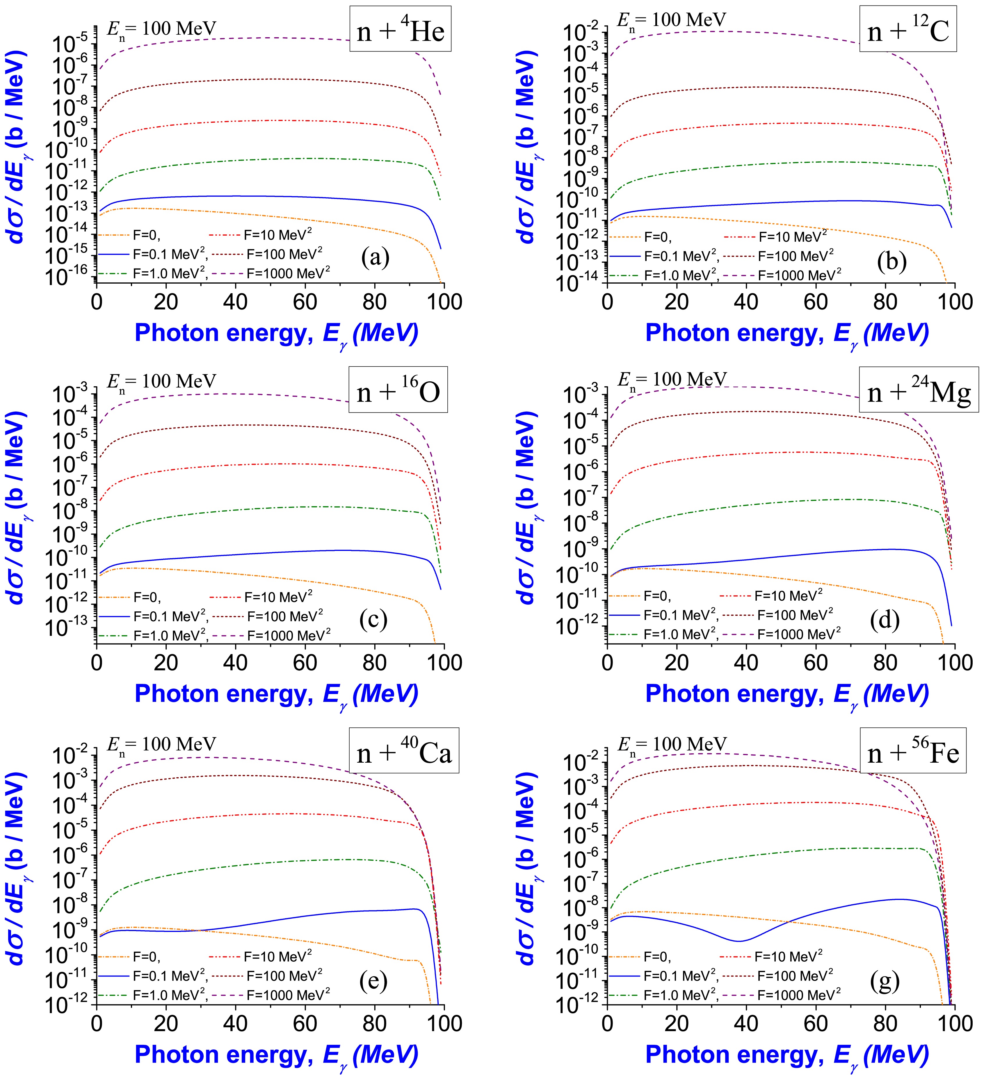

Figure 10.  (color online) Bremsstrahlung emission of photons in scattering of neutrons off ⁴He (a), ¹²C (b), ¹⁶O (c), ²⁴Mg (d), ⁴⁰Ca (e), and ⁵⁶Fe (g) nuclei inside dense stellar medium at neutron energy of $ E_{\rm n}=100 $ MeV. We calculate the spectra based on the incoherent matrix element $ M_{\Delta M} $ defined in Eqs. (4)–(6) and the matrix element $ M_{\rm star} $ defined in Eq. (24 at $ N = A(A-1) $. In calculations of normalization of full cross-sections, we take into account the ratios between the coherent and incoherent bremsstrahlung contributions given in the caption of Fig. 9).

After general analysis with the unified picture of emission of bremsstrahlung photons during scattering of protons and neutrons off nuclei given in Sec. II, we aim to analyze the influence of the structure of matter in neutrons stars on such emission. In this paper, we restrict ourselves by obtaining only the first preliminary estimations, while more accurate data should be obtained after careful analysis, as the structure of matter inside a dense stellar medium has been deeply studied (e.g., see Ref. [69] and references therein).

According to Ref. [46] (see p. 57 in that book), at a density of $ 4 \cdot 10^{11}\, {\rm g} / {\rm cm}^{3} $, the ratio between neutrons and protons reaches a critical value, and free neutrons, electrons, and nuclei co-exist inside (i.e., neutron drips are formed). When density is higher than $ 4 \times 10^{12}\, {\rm g} / {\rm cm}^{3} $, neutrons give larger pressure than electrons, and neutrons play a more important role than electrons. Thus, we take this condition as a starting point for analysis of bremsstrahlung during the scattering of neutrons off nuclei, where we will use the ⁵⁶Fe nucleus for calculations. Such a density in a star with density at the center of $ 10^{16}\, {\rm g} / {\rm cm}^{3} $ is in the external layer, close to the external surface of the star (see Fig. 11(a); this is at a distance of 10.63 km from the center of the star, and the radius of this star is 11.47 km).

However, nuclei in this space region of the star are located at very close distances. In approximation, one can estimate the distance between the two closest nuclei. Let us write density as

where $ n_{^{56}\text{Fe}} $ is the number of ⁵⁶Fe nuclei per unit volume, $ N_{^{56}\text{Fe}} $ is the number of ⁵⁶Fe nuclei per volume V, and $ m_{^{56}\text{Fe}} $ is the mass of an ⁵⁶Fe nucleus. From this formula, we find the average volume per nucleus as

Assuming that the nuclei inside such a dense medium are likely located in the most compact way, then the distance between the two closest nuclei can be estimated as

Based on this formula, for a density of $ 4 \times 10^{12}\, {\rm g} / {\rm cm}^{3} $, we calculate distance as $ d=28 $ fm. Here, consideration of the geometry and surface of a Wigner-Seitz cell will be more accurate in such estimations [69]. However, in this paper, we restrict ourselves to simple geometric schemes of location of nuclei.

Let us consider a neutron located between two closest nuclei. At some non-zero kinetic energy $ E_{\rm n} $, this neutron is incident (scattered) on one nucleus, i.e., we have the neutron-nucleus scattering process. On the grounds of QED, for non-zero kinetic energy of relative motion (of neutron and nucleus), there is a non-zero probability of emission of bremsstrahlung photons during such scattering.

Usually, for experiments on Earth, the bremsstrahlung cross-sections are calculated based on the square of the full matrix element of emission (see Eqs. (3)–(6)). Multipole expansion of the wave function of photons provides sufficiently accurate calculation of matrix elements of emission for different nuclear processes. Thus, in the framework of our formalism, we apply this expansion to the current task. As a result, each matrix element is represented as a multiplication of radial integrals and coefficients that describe the angular distribution of photon emission in the studied reaction. A main difficulty in this problem is in numeric calculations of radial integrals. These integrals can be written in general form as

where

and r is the distance between the neutron and nucleus center-of-mass. For conditions of experiments on Earth, to reach convergence in calculations of the bremss-trahlung spectra, we need to use $ R_{\rm max} $ at distances of atomic shells (more 10000 fm) or higher from the nuclear center. Thus, it is natural to suppose that other nuclei located at distances close to 28 fm should give strong changes in the full spectrum of bremsstrahlung emission. However, such a model is constructed based on space representation (in contrast to models constructed based on Feynman diagrams in momentum representation), and it provides an accurate means to estimate such an influence from other nuclei.

To perform such estimations, we calculate the spectra based on the integral $ I_{1} $ in Eq. (35), where we choose $ R_{\rm max,1}=d/2=14 $ fm. In such a case, corrections should be given after inclusion of another integral $ I_{2} $ in Eq. (35), where we choose $ R_{\rm min}=R_{\rm max,1}=14 $ fm and $ R_{\rm max}=10000 $ fm. One can compare the spectrum calculated based on only the first radial integral $ I_{1} $with the full spectrum with inclusion of this first integral $ I_{1} $ and addition of the second integral $ I_{2} $ also.

The results of such calculations are presented in Fig. 11 (b). In this figure, one can see that the spectrum based on the first radial integral $ I_{1} $ at $ R_{\rm max,1}=14 $ fm (red solid line) is very close to the spectrum based on the full radial integral I at $ R_{\rm max}=10000 $ fm (brown dash-dotted line). We also add calculated correction from the integral with boundaries $ R_{\rm min}=14 $ fm and $ R_{\rm max}=10000 $ fm to this figure multiplied by the factor $ 10^{10} $ (blue dash-double dotted line). This correction is extremely small, which confirms that the main part of bremsstrahlung emission is formed inside the space region up to 14 fm from the nuclear center. By such reasoning, we conclude that the influence of another nucleus (located farther than 28 fm from the studied nucleus) on emission of these bremsstrahlung photons is extremely small, and the obtained estimations are correct. This result indicates that the bremsstrahlung emission of photons from such nucleon-nucleus nuclear processes can even be studied for conditions inside neutron stars. It is supposed that such results can be applied for conditions of the inner crust of a neutron star (with even more accurate corrections based on the details of the structure there).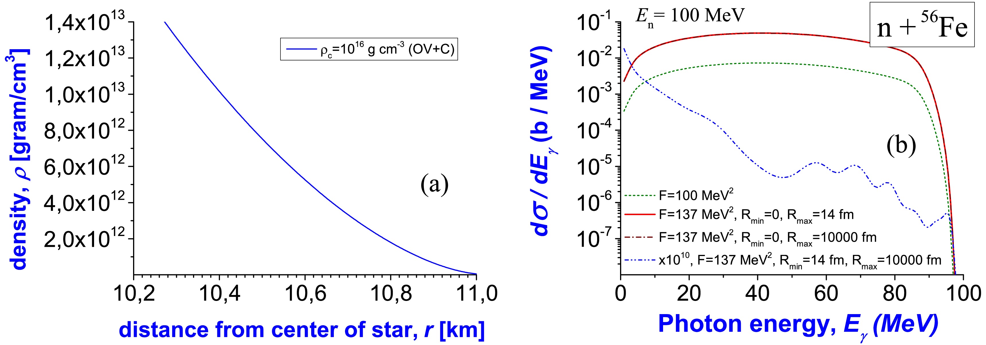

Figure 11.  (color online) [Panel a]: Density of matter inside star with density at center of $ 10^{16}\, {\rm g} / {\rm cm}^{3} $. The solution was obtained by the Oppenheimer–Volkoff equation with non-polytropic EOS; EOS is defined by Eqs. (2.3.5)–(2.3.6) in Ref. [46] for relativistic neutrons at $ \mu_{e}=1 $ (see p. 25–26 in that book)]. [Panel b]: Bremsstrahlung emission of photons in scattering of nucleons off ⁵⁶Fe nucleus at neutron energy of $ E_{\rm n}=100 $ MeV located at density $ 4 \cdot 10^{12}\, {\rm g} / {\rm cm}^{3} $. Here, the red solid line is the spectrum calculated based on the first radial integral $ I_{1} $ at $ R_{\max,1}=14 $ fm in Eq. (35), brown dash-dotted line is the spectrum calculated based on the full radial integral I at $ R_{\max}=10000 $ fm in Eq. (34), blue dash-double dotted line is the correction calculated based on the second radial integral $ I_{2} $ at $ R_{\max,1}=14 $ fm and $ R_{\max}=10000 $ fm in Eq. (35) and multiplied by a factor of $ 10^{10} $, and green dotted line is the full spectrum calculated based on the full radial integral at $ F=100\;\rm MeV^{2} $.

Quantum mechanics provides a natural basis for the study of such nuclear processes in dense matter. An effective way to describe such nuclear processes under the condition of dense matter can be obtained after unification of (1) the many-nucleon formalism on the structure of the nucleus and nuclear reactions based on quantum mechanics (new developments in line with Refs. [17−20]; see also Refs. [49−52]), (2) methods of quantum mechanics with high precision and tests (see method of Multiple Internal Reflections (MIR); also, there is method of phase functions in nuclear scattering), which describe processes of relative motion of two nuclei (or nuclear fragments) in nuclear scattering with the possible formation of a compound nuclear system and fusion (or opposite processes of nuclear decays), and (3) additional formalism describing the influence of dense medium on nuclear processes in a compact star.

In particular, the MIR method was initially constructed for α decays of nuclei and then applied for decays of nuclei with emission of protons. Later, it was generalized for the opposite process of the capture of α particles by nuclei (see Refs. [53, 54] and references therein). This method provides its own independent parameters of nuclear potentials for the studied fusion reactions with high (the highest) accuracy of agreement with available experimental information (e.g., see Ref. [53] for α-nucleus reactions, with details, comparison with alternative approaches, etc.). The method was investigated to study different stages and mechanisms of nuclear scattering (e.g., resonant and potential scattering are the simplest demonstrations). Then, that method was extended for fusion of nuclei in the case of close distance between those (like in lattice sites of compact star that do not exist Earth). The accuracy and effectiveness of this method were demonstrated in a study of the possibility of synthesis of new more heavy nuclei from close nuclei in neutron star at low energies (pycnonuclear reactions). This was presented as an example with isotopes of carbon in Refs. [77, 78].

Note that the accuracy of this method for the calculated cross sections of fusion is approximately $ 10^{-14} $, in comparison with existing alternative approaches of approximately$ 10^{-3} $ in best cases. Tests were developed to check and estimate calculations obtained by the MIR method and other methods (see Refs. [53, 54] and references therein for details). In Refs. [77, 78], there are demonstrations related to the study of the details of fusion for isotopes of carbon. Some new physical effects (which are not small and have not been studied by other approaches) were studied in Ref. [53] (under conditions of labs in Earth). In particular, in that publication, probabilities of fusion from experimental data were extracted, and new probabilities of fusion were predicted for new reactions with close isotopes for new experimental tests in the future. It is important to note that formalism of the MIR method is in direct connection with methods of the inverse scattering problem, which provides a basis for further study of nuclear forces in connection with experimental data. Thus, we estimate conditions of dense matter for which this can be naturally extended using the results of those publications and this paper. We believe this research provides a good perspective in the study of nuclear processes in dense matter and to extend that for collisions of nuclei with higher energies.

Emission of bremsstrahlung photons from nucleon-nucleon scattering is an important topic of research. It helps to understand many aspects of nucleon-nucleon interactions, the development of different relativistic models, etc. However, in nucleon-nucleus and nucleus-nucleus reactions, the many-nucleon problem is already important.

The role of many-nucleon processes (effects of many-body problem) in the calculation of cross-sections of emission of photons is larger when there are more nucleons in the nuclei. The easiest way to check this phenomenon is to study proton-nucleus scattering, where experimental data for bremsstrahlung are also obtained with high precision (we found that phenomenon in Refs. [55−57]; see also Ref. [10] and references therein).

Different aspects of many-nucleon effects can be explicitly described by the operator of emission of photons (and corresponding matrix elements) in the scattering of protons off nuclei composed of nucleons in unified formalism in frameworks of quantum mechanics. Here, both electric charges and (full) magnetic moments of protons and neutrons in nucleus-target and protons in the beam play important role. In the study of many-nucleon effects in general, magnetic moments of nucleons are essentially more important than the electric charges of these nucleons. In particular, magnetic moments of nucleons provide a basis for the incoherent emission of photons. It turns out that for nuclei of middle and heavy masses, the role of incoherent processes becomes significantly larger than the role of coherent processes (i.e., the case when emission of photons is produced due to relative motion (evolution) between nucleus-target as a whole object and proton beam in scattering). After inclusion of incoherent emission in the bremsstrahlung model, the understanding of full emission of photons in nuclear processes is changed significantly (shapes of cross-sections of full bremsstrahlung are changed even after possible re-normalizations of these spectra on the same experimental data). At the same time, for light nuclei (such as deuterium, isotopes of helium, beryllium; see Ref. [8]), the coherent emission is similar to the incoherent emission of photons.

One can even study the influence of clusters in nuclei on full bremsstrahlung emission (which characterizes the structure of these nuclei and is a pure phenomenon of the many-body quantum problem) using the many-nucleon formalism of quantum mechanics (see Refs. [8, 9]).

Thus, one can suppose that such many-nucleon effects are important in the study of different processes in the evolution of neutron stars. In particular, it will be interesting to know role of many-nucleon dynamics in producing the emission of photons in the cooling of neutron stars. Such mechanisms as incoherent processes in different nuclear processes with different isotopes of nuclei of different masses can be interesting to study. It would be useful to first obtain simple estimations providing a clear picture of this question. We would like to indicate the good perspective of this research direction in further study.

There is an interesting question in the study of neutrino emission in the cooling process of neutron stars, where many-nucleon dynamics in nuclear reactions can play an important role. To construct a model for such a study, we should solve some problems.

One problem is the unification of theory on the structure of nuclei and nuclear reactions strictly based quantum mechanics (in space representation; for example, see Refs. [17−20]) and a formalism describing the emission of neutrinos in reactions (described in QFT in a good way in momentum representation). We take the idea for the construction of this model from the study of the production of lepton-antilepton pairs (dileptons) in proton-nucleus scattering (heavy ion collisions) based on quantum mechanics (see Ref. [79]). The simplest process of production of dileptons can be described via the intermediate process of the exchange of virtual photons (between scattered nucleon and produced dilepton) based on the connection of hadronic and leptonic fluxes. Here, one flux describes the emission of a virtual photon from one nucleon of a nucleus-target or proton beam, and another flux describes the production of lepton pairs from a virtual photon. In the case of neutrino emission, one can generalize this formalism with a new implementation of weak fluxes describing the emission of a neutrino (in frameworks weak interaction theory).

Another unanswered question in this study is related to the observation of neutrinos emitted from nuclear reactions in such stars. We see good perspective in further development of a quantum mechanical model to study the emission of neutrinos in the cooling process in such stars.

One may think that bremsstrahlung emission from nuclear processes in stars is small. However, from our experience studying bremsstrahlung, such photons in nuclear reactions bring more rich and deep information about such nuclear processes (structure of nuclei, clusters, nuclear deformations, mechanisms of reactions, dynamical properties in scatttering, new properties of hypernuclei, even nuclear interactions, study of quarks in nuclear reactions, etc.; e.g., see Refs. [8−10] and references therein) than direct study of the reactions themselves, without inclusion of photons. Usually experimental cross-sections or probabilities of emitted bremsstrahlung photons are very small, but such investigations exist for a long time. For example, this even gives the possibility to construct a new type of microscopy to explore micro-world physics based on the analysis of bremsstrahlung emission. Such an attempt was performed by us, and now this idea has been accepted by the physical community (see Ref. [2]). In simple words, this is a transition from the study of some elementary processes with emission of photons known from textbooks on QED by many people to a principally new type of microscopy (constructed on the basis of bremsstrahlung analysis) to explore the more tiny microscopic structure of matter (without additional construction of new experimental facility, only using existing facilities and detectors for photons). Similarly, now we would like to find a more effective way to study the internal structure of stars, using emission of such photons and our previous investigations on the basis.

Before our study, many questions were unanswered. For example, it was not clear how the emission of bremsstrahlung photons changes with the density of matter in a star (now, we give some information and estimations with the help of the Referee).

We hypothesize that this model will give the possibility to measure densities of matter inside neutron stars if it is possible to measure the spectra of photons emitted from this object. A star can emit photons, but most photons emitted from reactions with higher intensities are not bremsstrahlung. These have essentially a different shape of spectrum with peaks. Peaks indicate processes of synthesis or other nuclear processes at some fixed photon energies. Another part of the spectrum of photons is of bremsstrahlung type. Such a spectrum looks like the spectra in Fig. 7 (spread, without peaks). Now, from the measured spectrum of photons, one can find the most probable value of kinetic energy of a scattered nucleon in nucleon-nucleus processes (see Figs. 8–10). Here, one can propose a simple formula for such estimations as $ E_{\rm p,n}^{\rm (kin)} = E_{\rm ph, max}/2 $ (here, $ E_{\rm p,n}^{\rm (kin)} $ is the estimated kinetic energy of the scattered nucleon, $ E_{\rm ph, max} $ is the energy of photons in the spectrum at the bremsstrahlung cross-section maximum). According to Eq. (25), the bremsstrahlung cross-section maximum indicates that the value of F that is related to the density of the stellar medium with the studied reaction and chosen EOS [see Figs. 8–10]. In this manner, one can try to extract information about the density of matter in compact objects from the possible measurements of photons. In this paper, we have constructed a basis for that investigation.

Another perspective is to apply that investigation to the collisions of heavy nuclei at close relativistic velocities (where high density of matter can be supposed compared to the saturation density of nuclear matter). Of course, to study that, we a require a working model, which should be tested on different tasks beforehand. One can suppose that bremsstrahlung photons emitted in such collisions can bring new information about dense nuclear matter of colliding nuclei or compound nuclear systems during collision. It will be interesting to investigate this line of research.

In this paper, the bremsstrahlung formalism [56, 57] (see Refs. [2, 3, 55, 61, 70−75]) for scattering of nucleons off nuclei was generalized for conditions of the dense medium of compact stars. For that, the nuclear model of deformed oscillator shells [49, 50, 52] was applied via new inclusion of the influence of stellar medium on the nucleons of nuclei. We obtained a unified picture of bremsstrahlung emission in the nucleon-nucleus scattering under the conditions of experiments on Earth and the dense medium of compact stars.

In frameworks of that formalism, the stellar medium does not affect the emission of photons in white dwarfs. In conclusion, we obtained a sufficiently accurate description of the emission of bremsstrahlung photons during nuclear reactions in the Sun, white dwarfs, and stars with similar densities. For neutron stars, the influence of stellar medium is essentially more intensive. This essentially changes the shape of the spectrum of bremsstrahlung photons. The most intensive emission is formed in the bowel of the star, while the smallest emission is from the periphery. One can obtain an approximate formula for the maximum probability of the emitted photons at half the energy of the scattered nucleon: $ E_{\rm ph} \simeq E_{\rm p} / 2 $ for protons. We estimated the emission of photons due to interactions of protons and neutrons with ⁸Be, ¹²C, ¹⁶O, ²⁴Mg, ⁴⁰Ca, ⁵⁶Fe inside a dense stellar medium (see Figs. 9 and 10). We found that the emission of bremsstrahlung photons in the scattering of neutrons of nuclei is not small. This is explained by the large contribution of incoherent processes due to the important role of magnetic moments of protons and neutrons in nuclei. All these results have been obtained at first time.

Electron-nucleus processes in the crusts of neutron stars produce bremsstrahlung emission. Nucleons of nuclei have magnetic moments and electrical charges. Investigations on bremsstrahlung in proton-nucleus scattering indicate a more intensive incoherent bremsstrahlung emission than a coherent one. This effect is small for light nuclei, but it is increased for heavy nuclei (e.g., the ratio in the proton-nucleus scattering of ⁵⁶Fe is $\dfrac{\sigma_{\rm incoh} (^{56}\text{Fe})}{\sigma_{\rm coh} (^{56}\text{Fe})} = 1.7592 \times 10^{5}$). Bremsstrahlung emission in the scattering of protons off nuclei were measured with high accuracy by the TAPS collaboration [60]. The plateau in these data cannot be described by the coherent bremsstrahlung only. Note that previously less accurate data indicating such a shape of spectra were obtained in Refs. [58, 59]. To explain measured data of bremsstrahlung, ratios between incoherent and coherent contributions were first extracted for those reactions [56]. Analysis of such data indicated essentially larger incoherent bremsstrahlung. Later, explicit formulas were obtained to predict such an incoherent bremsstrahlung. A similar situation also exists with electron nucleus scattering in the surface layer of stars (electrons also have magnetic momentum and non-zero spin). One can suppose that the inclusion of incoherent processes in the models of stars can change the ratios (between rates of emission and absorbtion) in such layers of stars. Thus, we see a perspective to check this idea carefully in further research.

The constructed model describes disintegration of nuclei for individual nucleons, starting from some critical distance between the nucleus and center of the star. The stellar medium acts on individual nucleons of a nucleus. Binding energy (which is negative for a nucleus in the external layer of a star) is increased at deeper locations of this nucleus in the star. Starting from some critical distance from the nucleus to the center of the star, the binding energy becomes positive (see Fig. 2). This means that the full energy of individual nucleons of the studied nucleus is already larger than the mass of this nucleus, i.e., we obtain an unbound system of nucleons, and the nucleus is disintegrated into nucleons. Such a phenomenon is observed in neutron stars (see Fig. 3) and is not observed in the white dwarfs.

The authors greatly appreciate Profs. V. S. Vasilevsky, M. I. Gorenstein, and A. V. Nesterov for their useful recommendations and interesting discussions concerning modern many-nucleons nuclear models and the physics of nuclear processes inside dense stellar media.

In this Appendix, we give a short review of the model of deformed oscillatoric shells (DOSs) (e.g., see Refs. [49−52]). The Hamiltonian of a nucleus as a system of A nucleons (in bound states) is defined in Eq. (9) as

and the Schrödinger equation is written as

Here, Ψ and E are the wave function and full energy of the nucleus, respectively, which are unknown and should be found.

The Hamiltonian in Eq. (A1) has potential two-nucleon nuclear and Coulomb interactions between all nucleons (i.e., this is a many-body problem of quantum mechanics). Ignoring the dependence of velocities of nucleons, the most general form of potential of nuclear interactions between two nucleons depends on three vectors: distance r between nucleons and two spins $ {\bf{s_{i}}} $, $ {\bf{s_{j}}} $ of nucleons with numbers i and j. This can be expressed via a potential (operator) with 6 different terms (e.g., see book [62], p. 555–559).

where

Here, $ {\bf{n}}_{ij} = ({\bf{r}}_{i} - {\bf{r}}_{j}) /r_{ij} $, $ r_{ij} = |{\bf{r}}_{i} - {\bf{r}}_{j}| $. The operator of exchange of two nucleons $ \hat{P} $ can be written via operators of isospin $ \hat{ {\boldsymbol{\tau}}_{i}} $, $ \hat{ {\boldsymbol{\tau}}_{j}} $ of two nucleons (e.g., see book [62], p. 550–551).

The potential $ \hat{V}(ij) $ can be rewritten in another form via four potentials $ \hat{U}_{2S+1, 2T+1} $, where $ T=0,1 $ and $ S=0,1 $ are eigenvalues of operators of full isospin and the spin of system of two nucleons, respectively (e.g., see book [62], p. 559). In the DOS model, this potential is transformed into the following form:

where the spin and isospin operators of exchange are (e.g., see Ref. [76], p. 24, 55; Ref. [62], p. 289)

Using the DOS model, the full energy of the nucleus and unknown wave function are calculated as a solution of the many-body problem in the first order of perturbation theory in quantum mechanics. One can find the next corrections (it is known that the second correction improves the agreement between calculated binding energies and their experimental values for a wide region of nuclei, but we do not focus on this in this paper). Under first-order perturbation theory, we calculate energy as

where $ \Psi_{0} $ is an unperturbative wave function. In the DOS model, this wave function is defined as

Here, $ \beta_{A} $ is the set of numbers $1, 2, \cdots, A$ of nucleons in the nucleus, and $ \psi_{\rm nucl} (\beta_{A}) $ is the many-nucleon function dependent on nucleons of the nucleus. The summation in Eqs. (A8) is performed over all $ A! $ permutations of coordinates or states of nucleons. The one-nucleon function $ \psi_{\lambda_{s}}(s) $ represent the multiplication of space and spin-isospin functions as $ \psi_{\lambda_{s}} (s) = \varphi_{n_{s}} ({\bf{r}}_{s})\, \bigl|\, \sigma^{(s)} \tau^{(s)} \bigr\rangle $, where $ \varphi_{n_{s}} $ is the space function of the nucleon with number s, $ n_{s} $ is the number of state of the space function of the nucleon with number s, and$ \bigl|\, \sigma^{(s)} \tau^{(s)} \bigr\rangle $ is the spin-isospin function of the nucleon with number s. The one-nucleon space function is formulated as an eigenfunction of the 3D harmonic oscillator as

where $ H_{n_{x}} $, $ H_{n_{y}} $, and $ H_{n_{z}} $ are the Hermitian polynomials, and a, b and c are oscillator lengths. It is supposed that all oscillator lengths are unknown (for each nucleus), and these required parameters are found from the condition of minimum full energy of the nucleus while varying these parameters. In this way, the minimum of full energy (related to binding energy) and all required parameters for the wave function are found for each nucleus.

Thus, in the DOS model, interacting potential is dependent on spin and isospin operators, nuclear energy is calculated analytically for even-even nuclei (where both cases $ N \ne Z $ and $ N=Z $ are included). The matrix element in Eq. (10) in the manuscript for nuclear energy is obtained through calculation of the wave function in the form of Eqs. (A8)–(A9) and potential in the form of Eqs. (A5)–(A6) and summation over all spin and isospin states. This formalism can be extended (developed) for nuclei with an odd number of protons or/and neutrons (this case is not analyzed in this manuscript).

The saturation property of nuclear matter is also taken into account, which gives additional relations between components of potential (see logic in book [62], p. 560). Taking these properties into account and also from the analysis of meson theories for one-pion exchange, one can obtain (see Eq. (1) in Ref. [49])

For calculation, this is written as

where $ V_{t}=72.5 $ MeV, $ \mu_{t}=1.47 $ fm, $ V_{s}=39.15 $ MeV, and $ \mu_{s}=1.62 $ fm. Potentials $ U_{31} $ and $ U_{13} $ in Eq. (A11) with such parameters are obtained from good description of experimental data for scattering lengths and effective radii in nucleon-nucleon scattering.

The full energy of each nucleus is calculated by varying the oscillator lengths of one-nucleon space functions. Varying such parameters, one can obtain the minimum of full energy. This point indicates the most stable state of the nucleus. This state is chosen as the ground state for the analyzed nucleus, and oscillator lengths and full energy of nucleus (and binding energy) are found. Such a procedure is stable, as minima of energies are clear for each nucleus. As a demonstration, Fig. 2 and Fig. 3 show the results for nuclei from ⁴He up to ⁵⁶Fe. This procedure also works if additional influence from the stellar medium is added to the model (this is a new aspect of the DOS model that has not been studied previously).

From Eq. (12), we calculate the proton and neutron densities for isotopes of ^4,6,8He and ^8,10Be as follows:

where

One can see that the proton and neutron densities are the same for ⁴He, ⁸Be nuclei and different for ⁶He, ⁸He, ¹⁰Be nuclei. Also, we have the following properties:

Here, we find the potential energy of two-nucleon nuclear interactions for a ⁶He nucleus based on the matrix element in Eq. (10) and found densities in Eq. (A12). After calculations, we obtain the following:

where

where we use the following notations (with change of indexes t and s):

From the solutions above, one can see that (1) only ⁴He is spherical in the ground state, while other nuclei are deformed; (2) ⁶He and ⁸Be nuclei are axially symmetric in the ground state, while ⁸He and ¹⁰Be are fully deformed. Further calculations of minima of full energy of these nuclei confirm such a logic.

Under spherically symmetric approximation ($ a = b = c $), we obtain

where

In this section, we find the correction of energy of the nucleus due to the influence of stellar medium (18):

Substituting Eq. (17) into this formula and taking into account the same action of force $ {\bf{F}}_{P}(R) $ for each nucleon, we obtain

We use the property

Here, summation is performed over all states for the given nucleus configuration (denoted by indexes m and k). All nucleons are numeberd by indexes i and j. We use the following representation for the one-nucleon wave function:

where $ \varphi_{n_{s}} $ is the space function of the nucleon with number s, $ n_{s} $ is the number of state of the space function of the nucleon with number s, and $ \bigl|\, \sigma^{(s)} \tau^{(s)} \bigr\rangle $ is the spin-isospin function of the nucleon with number s. For operator $ \hat{V}\, ({\bf{r}}_{i}, {\bf{r}}_{j}) $ acting on space functions for two nucleons only, we calculate the matrix element

where orthogonalization properties of spin and isospin functions are used as follows:

In particular, for ⁴He, Eq. (B6) is simplified as follows:

and we obtain

where Eq. (A13) for $ F_{0} ({\bf{r}}_{i}, {\bf{r}}_{j}) $ is used. For correction of energy, from Eq. (B1), we obtain

In the spherically symmetric case ($ a=b=c $), we calculate the integral as

and obtain the solution

In this section, we describe some aspects of the folding approach we use and its connection to the microscopic approach for nucleon-nucleus scattering. Definitions of the folding and cluster models in nucleon-nucleus and nucleus-nucleus scattering are given in Ref. [8] (see Eqs. (1) and (2) in that paper), where determination of folding potential is described by Eqs. (9)–(31) in Ref. [8].

In the folding approach, the key element is representation of the full wave function for nucleon-nucleus scattering in a more approximated form than in the fully microscopic formalism. Following to this formalism, the full wave function of the proton-nucleus scattering is written as $ \Psi = \Phi ({\bf{R}}) \cdot \Phi_{\rm p - nucl} ({\bf{r}}) \cdot \psi_{\rm nucl} (\beta_{A}) $ (also following the formalism in Ref. [56] for proton-nucleus scattering, see Sect. II.B, Eqs. (10)–(13)); the many-nucleon structure of the nucleus is described in Ref. [55]). Here, $ \Phi ({\bf{R}}) $ is the function describing the motion of the center-of-mass of the full nuclear system in the laboratory frame; $ \Phi_{\rm p - nucl} ({\bf{r}}) $ is the function describing relative motion of the scattered proton concerning the nucleus (without description of internal relative motions of nucleons in the nucleus); $ \psi_{\rm nucl} (\beta_{A}) $ is the many-nucleon function of the nucleus, defined in Eq. (12) of Ref. [56] based on the one-nucleon functions $ \psi_{\lambda_{s}}(s) $; and $ \beta_{A} $ is the set of numbers $1,2, \cdots, A$ of nucleons of the nucleus. One-nucleon functions $ \psi_{\lambda_{s}}(s) $ represent the multiplication of space and spin-isospin functions as $ \psi_{\lambda_{s}} (s) = \varphi_{n_{s}} ({\bf{r}}_{s})\, \bigl|\, \sigma^{(s)} \tau^{(s)} \bigr\rangle $, where $ \varphi_{n_{s}} $ is the space function of the nucleon with number s, $ n_{s} $ is the number of state of the space function of the nucleon with number s, and $ \bigl|\, \sigma^{(s)} \tau^{(s)} \bigr\rangle $ is the spin-isospin function of the nucleon with number s. Definitions are also given in Ref. [11].

In our paper, we assume an approximated form of the function $ \Phi_{\bar{s}} ({\bf{R}}) $ a before and after emission of photon as ($ \bar{s}=i $ is for state before emission of photon, and $ \bar{s}=f $ is for state after emission of photon)

where $ {\bf{K}}_{i} $ and $ {\bf{K}}_{f} $ are moments of the full nucleon-nucleus system in states before and after emission of a photon in the laboratory frame, respectively.

In the description of the structure of the nucleus in this problem, we use the DOS model instead of part of the formalism in Refs. [8, 9]. This DOS model gives a clearer analysis of the structure of nuclei, provides calculations of the wave function $ \psi_{\rm nucl} (\beta_{A}) $ of the nucleus, binding energy, deformations of different isotopes of light nuclei (which were previously compared with existeing experimental data), and allows us to include the influence of the stellar medium on the nucleus. It also provides sufficiently close calculations of the properties of light nuclei but without clusters inside these nuclei. For many calculations of ⁴He and other light nuclei, this is convenient, and we use it. It speeds up many calculations (even some analytical). The bremsstrahlung formalism of the DOS model provides wave functions that are important for the determination of form factors in the calculation of cross-sections of bremsstrahlung.

Note that all wave functions should be found from numerical solutions of the Schrodinger equation for nucleon-nucleus scattering with the given nucleon-nucleon potentials. However, in the problem of emission of bremsstrahlung photons in this reaction, these wave functions are already used, so we develop a formalism for the operator of photon emission (or different contributions to it, such as coherent and coherent contribution), and we numerically calculate the matrix elements of bremsstrahlung emission based on the previously found wave functions and this operator of emission. In practical calculations of bremsstrahlung spectra, we need to know the wave functions of relative motion between the scattered nucleon and nucleus $ \Phi_{\rm p - nucl} ({\bf{r}}) $, which are calculated numerically in terms of the kinetic energy $ E_{T} $ of relative motion between these two objects. The exact formulas are $ E_{T} = \dfrac{A}{A+1}\, E_{\rm p} $ and $ E_{\rm cm} = \dfrac{1}{A+1}\, E_{\rm p} $, where $ E_{\rm p} $ is kinetic energy of the scattered proton in the laboratory frame. However, for problems where one object in scattering is a nucleon, the approximation $ E_{T} \simeq E_{\rm p} $ is sufficient (we used this in calculations in this paper).

The formalism (in compact form) of calculations of matrix elements of bremsstrahlung for proton-nucleus scattering in the folding approximation is presented in Ref. [10] and its Supplementary Material [11] (here, there is a reference list for more details with explanations, where the required definitions are given). In particular, in the Supplementary Material [11], the formalism of inclusion of each function $ \Phi ({\bf{R}}) $, $ \Phi_{\rm p - nucl} ({\bf{r}}) $, and $ \psi_{\rm nucl} (\beta_{A}) $ in the calculation of bremsstrahlung cross-sections in the nucleon-nucleus scattering is presented.

The equation of equilibrium for a star under Newtonian gravity has form (see Eq. (1.2), p. 19, [14])

This can be rewritten as

Also, we should take into account the equation of continuity of mass (e.g., see Eq. (1.3) in Ref. [14], p. 19:

Substituting this into Eq. (D2), we obtain (see Eq. (1.4) in Ref. [14], p. 21)

Let us write the polytropic dependence of pressure P on density ρ as

where K is constant, and γ is the polytropic index. Stars with such EOS are called polytropic (see Ref. [14], p. 19). Using this, Eq. (D4) is transformed as

Now, we introduce unitless density θ and dimension ξ as

where $ \rho_{\rm c} $ is density at center of the star, n is the polytropic index, and $ R_{0} $ is a parameter. Substituting these into Eq. (D6), after derivation, we obtain

For choice

we obtain the Lane-Emden equation of equilibrium of a polytropic star:

The Tolmann-Oppenheimer-Volkoff (TOV) equation is

and the equation of conservation of mass is

Also, we use the polytropic EOS as

Here, K is constant. We obtain

Substituting this formula into (D11), we find

Now, we introduce unitless density and distance as

and Eq. (D15) is transformed as

Thus, we obtain the following system of equations based on the TOV formalism:

This system of equations can be rewritten in compact form as:

Here, new coefficients are introduced as follows:

This system is solved numerically under initial conditions of $ \theta(0) = 1 $, $\dfrac{{\rm d}\theta(0)}{{\rm d}\xi} = 0$. Also, $ \xi^{*} $ is the unitless radius of star, which is found from the condition of zero density at boundary $ \theta(\xi^{*}) = 0 $, and the radius of the star is $ r_{star} = \xi^{*}\, R_{0} $. To solve this system of equations, the parameters $ R_{0} $ and K must be defined. A simple formalism of calculations of these parameters is presented in Appendix D.3 (see Eqs. (D34) and (D35)).

The system of equations (D19) can be rewritten in form of one differential equation, expressing the function θ in terms of m. At first, from the second equation of Eq. (D19), we find the function θ and its derivative as

Substituting these solutions into the first formula in Eqs. (D19), we obtain

Mass m is calculated in units of MeV in numerical calculations.

We follow the formalism in Ref. [14] (see p. 29–34 in that book). Let us consider the equation of state of completely degenerate electrons. Because electrons are fermions with a half-integer spin of $ 1/2 $, only one electron with a given spin in a phase space cell can be there. The distribution function at complete degeneracy $ f_{e} (p) $ is given by a shelf in the region $ 0 < p < p_{fe} $, where the maximal momentum of the electrons $ p_{fe} $ is called the Fermi momentum. The volume of one phase space cell is $ (2 \pi, \hbar)^{3} $. Electrons occupy a spherical volume of $ V_{\rm ph} $ with a radius of $ p_{fe} $ in the phase space, and

Note that, in one cell of the phase space, there are two electrons with spins of $ 1/2 $ and $ - 1/2 $. Therefore, the concentration of completely degenerate electrons can be written as

This formula defines the dependence of $ p_{fe} $ on the concentration of $ n_{rm e} $:

The isotropic pressure of electrons $ P_{\rm e} $ is determined by the momentum flux as

A relativistic relation between velocity and momentum is used here:

The energy of a unit of volume $ \varepsilon_{rm e} $ is written in the same way as Eq. (D26). The total energy of one electron is equal to $ \sqrt{p^{2} + m_{\rm e}^{2} c^{2}} $. The maximal kinetic energy of one electron in degenerate matter (Fermi energy) is

The integral in Eq. (D26) cannot be derived easily. However, within non-relativistic and ultra-relativistic limits, the relations are quite simple:

The concentration of electrons due to electroneutrality is expressed in terms of the density of matter

where $ mu_{\rm e} $ is the number of nucleons per electron. For hydrogen, $ \mu_{\rm e} = $1. In a substance consisting of helium, carbon, and oxygen, we have $ \mu_{\rm e} = 2 $. From Eq. (D30), one can see that in non-relativistic white dwarfs, the matter has a polytropic index of $ \gamma = 5/3 $ ($ n = 3/2 $). For such stars, the mass increases with increasing central density as $ M_{\rm wd} \sim \sqrt{\rho_{c}} $ (see Ref. [14], p. 32).

At high densities in the ultra-relativistic limit, the polytropic index is $ \gamma = 4/3 $ ($ n = 3 $), and the mass of star in equilibrium with increasing density tends to the Chandrasekhar limit (see Eq. (2.4), p. 32, Ref. [14]).

Let us write down the found EOS in polytropic form as

To do this, convert Eq. (D29) while taking concentration into account:

Non-relativistic approximation ($ p_{fe} \ll m_{\rm e} c^{2} $, $ \gamma = 5/3 $, $ n = 3/2 $):

Ultrarelativistic approximation ($ p_{fe} \gg m_{\rm e} c^{2} $, $ \gamma = 4/3 $, $ n = 3 $):

Calculations for $ ^{4}\text{He} $ give ($ \mu_{e} (^{4}\text{He}) = 2 $)

Also, we have

We are interested in how the emission of photons changes after a change of parameter n in politropic EOS. Such calculations for $ p + $⁴He in a dense stellar medium at $ n=3/2 $ are shown in Fig. D1.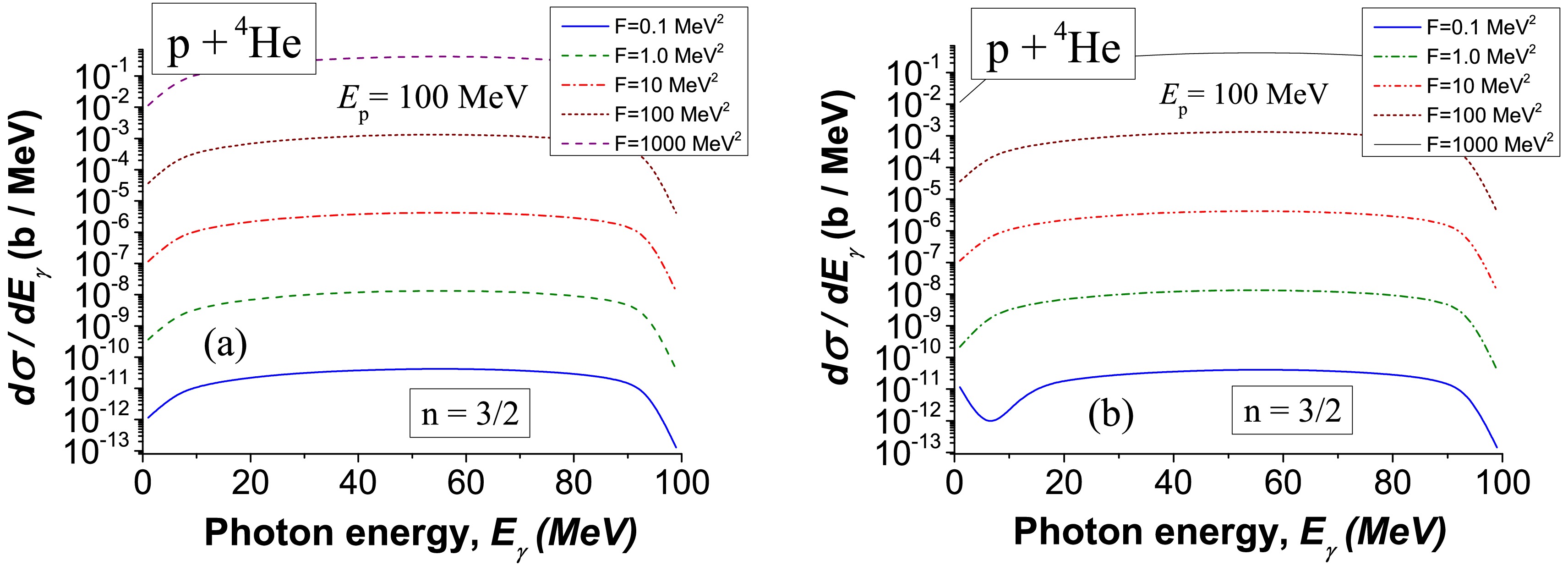

Figure D1.  (color online) Bremsstrahlung emission of photons in the scattering of protons off ⁴He nuclei inside a star at a proton energy of $ E_{\rm p}=100 $ MeV at polytropic index $ n=3/2 $. We calculate the spectrum based on the leading matrix element $ M_{p}^{(E,\, {\rm dip},0)} $, which gives the largest contribution to the full spectrum according to analysis in Refs. [56, 57]. The contribution based on the matrix element $ \langle \Psi_{f} |\, \Delta \hat{H}_{\gamma} |\, \Psi_{i} \rangle $ in Eq. (23) (a) and full spectrum based on the matrix element $ \langle \Psi_{f} |\, \hat{H}_{\gamma} |\, \Psi_{i} \rangle_{\rm star} $ in Eq. (23) (b) are shown here. Comparing these calculations with the results in Fig. 8 obtained at $ n=3 $, for the same density, we see that at $ n=3/2 $, the emission of photons in the stellar medium approximately 100 times greater than that under similar conditions at $ n=3 $. To conclude, we see that the EOS has an essential influence on the calculations of cross-sections of photon emission in a dense medium.