Probing heavy charged Higgs bosons at gamma-gamma colliders using a multivariate technique

A neutral Higgs boson with a mass of approximately 125 GeV was discovered by the ATLAS and CMS collaborations at the Large Hadron Collider (LHC) in 2012, and its properties were consistent with the prediction of the Standard Model (SM) Higgs boson [1−3]. Within the SM framework, gauge bosons acquire their masses through the Brout–Englert–Higgs mechanism through the concept of electroweak symmetry breaking (EWSB). The SM of particle physics does not provide any indications of charged Higgs bosons. However, theories beyond the SM propose the existence of charged Higgs bosons and are frequently incorporated into theoretical frameworks, such as Two-Higgs-Doublet Models (2HDMs), supersymmetric models, composite Higgs models, grand unified theories, and axion models. Among all these beyond SM theories, the 2HDM is very important owing to its structural relevance to many new physics models such as the Minimal Supersymmetric Standard Model (MSSM) [4, 5], composite Higgs models, and axion models [6, 7]. Depending on the couplings with quarks, the types of 2HDMs predict different properties and interactions for charged Higgs bosons. A charged Higgs boson would be a more massive counterpart to the SM $ W^{\pm} $ and Z bosons, which are carriers of the weak force. The Higgs sector in the 2HDM has been extended to incorporate other degrees of freedom that include the prediction of five Higgs candidates of the MSSM [8, 9]. From these five Higgs boson candidates, two of them are CP even neutral states h, H, one of them is CP odd A state, and the remaining two are charge Higgs states $ H^\pm $. The discovery of any new scalar Higgs boson, either neutral or charged, will be a strong hint towards the physics beyond the SM of particle physics and the immediate sign of an extended Higgs sector.

At the photon-photon ($ \gamma-\gamma $) collider, which is a proposed experimental facility at the International Linear Collider (ILC), high-energy electron-positron beams will be collided, which will result in the production of highly energetic photons. The basic concept behind this is that these highly energetic photons will collide with each other and provide a unique opportunity to study many phenomena such as the production of charged Higgs or other new-physics processes.

Therefore, future $ e^{+}e^{-} $ and $ \gamma\gamma- $ colliders, with high energy and luminosity values, will offer significant potential for discovering charged Higgs bosons. The output rate at a $ \gamma\gamma- $ collider could exceed that of $ e^{+} e^{-}- $ collisions at the tree level. In the 2HDM, the $ e^{+} e^{-} \rightarrow H^{+} H^{-} $ process has been analyzed at the tree level, whereas the $ \gamma\gamma \rightarrow H^{+} H^{-} $ process has only been studied at the Born level with Yukawa corrections [10, 11]. The primary channels for the pair production of charged Higgs bosons at linear colliders are $ e^+ e^- \rightarrow H^+ H^- $ and $ \gamma\gamma \rightarrow H^+ H^- $. Generally, the cross-section for $ e^+ e^- \rightarrow H^+ H^- $ is suppressed by s-channel contributions at high energies, which can result in a larger production rate for the $ \gamma\gamma \rightarrow H^+ H^- $ mode compared with the $ e^+ e^- $ collision mode. However, the s-channel contributions can be enhanced through specific couplings relative to the $ \gamma\gamma $ process. The scattering process $ e^+ e^- \rightarrow H^+ H^- $ has been extensively studied, with the incorporation of one-loop corrections within the frameworks of both the 2HDM and MSSM. Conversely, the scattering process $ \gamma\gamma \rightarrow H^+ H^- $ has also been analyzed at the one-loop level.

This paper focuses on the multivariate analysis of the production of charged Higgs bosons at the photon-photon collider at the International Linear Collider (ILC). Three benchmark points (BPs) are selected for numerical examination, each with a $ \mathcal{CP} $-even scalar mass of $125\; {\rm GeV}$ and couplings consistent with the known Higgs boson. These points are derived from "non-alignment", "low-$ m_{H} $", and "short-cascade" scenarios and are accurately delineated within the constraints of current experimental data, and they are fully consistent with theoretical constraints [12]. The cross-section is scanned for the plane $ (\phi^{0},\sqrt{s}) $, where $ \phi^{0} $ is $ h^{0} $ for the low-$ m_{H} $ scenario and $ H^{0} $ for non-alignment and short-cascade scenarios. Additionally, the polarization effect is discussed for all scenarios.

Two scalar doublets are used to acquire masses for gauge bosons and fermions after obtaining their vacuum expectation values (VEVs). The Lagrangian is given by

where $\mathcal{L}_{\rm Scalar}$ is the Lagrangian for the two scalar doublets including kinetic blueenergy and scalar potential terms. The $ Z_{2} $ symmetry is incorporated to ignore the Flavour Changing Neutral currents (FCNCs); thereafter, the transformation for the even state is $ \Phi_{1}\rightarrow +\Phi_{1} $, and that for the odd state is $ \Phi_{2}\rightarrow -\Phi_{2} $. To keep $\mathcal{L}_{\rm Yukawa}$ invariant for fermions under $ Z_{2} $-symmetry, we couple the fermions with one scalar field:

In Eq. (2), $ \Phi_{u,d,\ell} $ is either $ \Phi_{1} $ or $ \Phi_{2} $; therefore, based on the discrete symmetry of fermions, the 2HDM is classified into four types: Types I, II, III, and IV. This study focuses on a $ \mathcal{CP} $-conserving 2HDM. If we assume that in the 2HDM, the electromagnetic gauge symmetry is present to perform $S U(2)$ rotation on two doublets for alignment of VEVs of two doublets with $S U(2)$, $v=246\; {\rm GeV}$ will occupy one neutral Higgs doublet [13]. The two complex doublets $ \Phi_{1} $ from the SM and $ \Phi_{2} $ from EWSB are used to construct the 2HDM. The scalar potential under the $S U(2)_{L}\; \otimes\; U(1)_{Y}$ invariant gauge group is defined as

In Eq. (3), the quartic coupling parameters are $ \lambda_{i} $ $(i=1,2,3,\cdots,7)$ and the complex two doublets are $ \Phi_{i} \; (i=1,2) $. The hermiticity of the potential forces $ \lambda_{1,2,3,4} $ is real, whereas $ \lambda_{5,6,7} $ and $ m^{2}_{12} $ can be complex. The Paschos-Glashow-Weinberg theorem suggests that a discrete $ Z_{2} $-symmetry can explain certain low-energy observables [14, 15]. Utilizing this symmetry is crucial to effectively preventing any possibility of FCNCs occurring at the tree level. The $ Z_{2} $-symmetry requires that $ \lambda_{6}=\lambda_{7}=0 $ and $ m^{2}_{12}=0 $. If this is not allowed, i.e., $ m^{2}_{12} $ is non-zero, then the $ Z_{2} $-symmetry is softly broken for the translation of $ \Phi_{1}\rightarrow +\Phi_{1} $ and $ \Phi_{2}\rightarrow -\Phi_{2} $. The $ Z_{2} $ assignments produce four 2HDM types, as mentioned earlier [16, 17]. Table 1 demonstrates how fermions bind to each Higgs doublet in the permitted types when flavor conservation is naturally observed.

Type	$ u_{i} $	$ d_{i} $	$ \ell_{i} $
I	$ \Phi_{2} $	$ \Phi_{2} $	$ \Phi_{2} $
II	$ \Phi_{2} $	$ \Phi_{1} $	$ \Phi_{1} $
III	$ \Phi_{2} $	$ \Phi_{2} $	$ \Phi_{1} $
IV	$ \Phi_{2} $	$ \Phi_{1} $	$ \Phi_{2} $

Table 1.  In 2HDMs with $ Z_{2} $-symmetry, Higgs doublets $ \Phi_{1} $,$ \Phi_{2} $ couple to u-type and d-type quarks, as well as charged leptons.

This work focuses only on Type-I and Type-II 2HDMs; in Type-I, only the $ \Phi_{2} $ doublet interacts with both quarks and leptonblues similar to the SM. In Type-II, $ \Phi_{1} $ couples with d-type quarks and leptons, whereas $ \Phi_{2} $ couples only with u-type quarks.

After the EWSB of $S U(2)_{L}\, \otimes U(1)_{Y}$, the scalar doublet's neutral components cause the VEV to be $ v_{j} $.

where $ \rho_{j} $ and $ \eta_{j} $ are real scalar fields. The quartic coupling parameters $ \lambda_{1}-\lambda_{5} $ and mass terms $ m^{2}_{1} $, $ m^{2}_{2} $ are considered physical masses of $ m_{h},m_{H},m_{A},m_{H^{\pm}} $ with $ \tan\beta=\dfrac{v_{1}}{v_{2}} $ and mixing term $ \sin(\beta-\alpha) $. After $ Z_{2} $-symmetry is broken softly, the parameter $ m^{2}_{12} $ is given by

where the last equality is only for the tree level. By considering $ \lambda_{6} $ and $ \lambda_{7} $ equal to zero concerning $ Z_{2} $-symmetry, $ m^{2}_{12} $, $ \tan\beta $, and the mixing angle $ \alpha $ with four Higgs masses, it is sufficient to compute a complete model on a physical basis. Therefore, based on this, seven independent free parameters are used to explain the Higgs sector in the 2HDM. The terms $ m^{2}_{1} $ and $ m^{2}_{2} $ are given in the form of other parameters:

The phenomenology is dependent on the mixing angle with the angle $ \beta $. In the limit where the $ \mathcal{CP} $-even Higgs boson $ h^{0} $ acts as the SM Higgs boson, it approaches the alignment limit, which is most favored by experimentalists if $ \sin(\beta-\alpha)\rightarrow 1 $ or $ \cos(\beta-\alpha)\rightarrow 0 $. $ H^{0} $ acts as gauge-phobic Higgs boson such that its coupling with vector bosons $ Z/W^{\pm} $ is much more suppressed, but when $ \cos(\beta-\alpha)\rightarrow1 $, $ H^{0} $ behaves similar to an SM Higgs boson. For the decoupling limits, $ \cos(\beta-\alpha)=0 $ and $ m_{H^{0}, A^{0}, H^{\pm}}>>m_{Z} $; therefore, at this limit, the interaction of $ h^{0} $ with SM particles completely appears similar to the couplings of the SM Higgs boson that contain coupling $ 3h^{0} $.

The theoretical restrictions of potential unitarity, stability, and perturbativity compress the parameter space of the scalar 2HDM potential. The vacuum stability of the 2HDM limits $ V_{\rm 2HDM} $. Specifically, $ V_{\rm 2HDM} \geq 0 $ must be satisfied for all $ \Phi_{1} $ and $ \Phi_{2} $ directions. As a result, the following criteria are applied to the parameters $ \lambda_{i} $ [18, 19]:

Another set of constraints enforces the perturbative unitarity to be fulfilled for the scattering of longitudinally polarized gauge and Higgs bosons. Moreover, the scalar potential must be perturbative by demanding that all quartic coefficients satisfy $ |\lambda_{1,2,3,4,5} | \leq 8\pi $. The global fit to EW requires $ \Delta\rho $ to be $ \mathcal{O}(10^{-3}) $ [20]. This prevents significant mass splitting between Higgs bosons in the 2HDM and requires that $ m_{H^{\pm}} \approx m_{A}, m_{H} $, or $ m_{h} $.

In addition to the theoretical restrictions mentioned above, 2HDMs have been studied in previous and continuing experiments, such as direct observations at the LHC or indirect B-physics observables. Consequently, numerous findings have been obtained, and the parameter space of the 2HDM is now constrained by all results obtained. In the Type-I 2HDM, the following pseudoscalar Higgs mass regions have been excluded by the LHC experiment: 310 $ \le m_{A} \le $ 410 GeV for $ m_{H} $ = 150 GeV, 335 $ \le m_{A} \le $ 400 GeV for $ m_{H} $ = 200 GeV, and 350 $ \le m_{A} \le $ 400 GeV for $ m_{H} $ = 250 GeV with $ \tan\beta = 10 $[21]. Furthermore, the $ \mathcal{CP}- $odd Higgs mass is bounded as $ m_{A} \ge $ 350 GeV for tan$ \beta \le $ 5 [22], and the mass range 170 $ \le m_{H} \le $ 360 GeV with tan$ \beta \le $ 1.5 is excluded for Type-I [23].

The $ H^{\pm} $ mass is constrained by experiments at the LHC and previous colliders, as well as B-physics observables. The BR($ b\rightarrow s\gamma $) measurement limits the charged Higgs mass in Type-II and -IV 2HDMs with $ m_{H^{\pm}} \geq $ 580 GeV for tan$ \beta\geq $ 1 [24, 25]. In contrast, the bound is significantly lower in Type-I and -III 2HDMs [26]. With tan$ \beta\geq $ 2, the $ H^{\pm} $ in Type-I and -III 2HDMs can be as light as 100 GeV [27, 28] while satisfying LEP, LHC, and B-physics constraints [29−33].

In our study, we focus on electron-positron ($ e^+e^- $) collisions, where the center-of-mass energy, represented as s, is crucial to understanding these interactions. Notably, during these collisions, photons can be emitted owing to bremsstrahlung effects and other mechanisms. These emitted photons may subsequently engage in interactions that mimic photon-photon ($ \gamma\gamma $) collisions. While such photon interactions can facilitate the production of additional particles, their energy levels are often unpredictable, making them less controllable than the highly precise and defined energy present in $ e^+e^- $ collisions. Therefore, our analysis primarily emphasizes the controlled conditions offered by electron-positron collisions while also acknowledging the potential contributions of radiated photons to particle production.

We have taken three scenarios [12]: non-alignment, short cascade, and low-$ m_{H} $. All of these are taken for a $ \mathcal{CP}- $even scalar with a mass of $ 125\; {\rm{GeV}} $, and couplings are well arranged with the observed Higgs boson. Additional Higgs boson searches leave a considerable portion of their parameter space unconstrained, emphasizing the need for further investigation. The potential stability, perturbativity, and unitarity for each BP were validated using $ \mathtt{2HDMC\;1.8.0} $ [33].

These benchmark scenarios, shown in Table 2, are created using a hybrid approach, where the input parameters are specified as $ (m_{h},m_{H}, \cos(\beta-\alpha), \tan\beta, Z_{4}, Z_{5}, Z_{7}) $ with a softly broken 2HDM of $ Z_{2}- $symmetry, where $ Z_{4,5,7} $ are quartic couplings in the Higgs basis of $ \mathcal{O} $(1). The mass of charged and pseudoscalar Higgs bosons in this basis is obtained as

Scenario	${\boldsymbol{ {m_{h^{0} } } }}$/GeV	${\boldsymbol{ {m_{H^{0} } } }}$/GeV	$ {\bf{{c_{\beta-\alpha}}}} $	${\boldsymbol{Z_{4} } }$	${\boldsymbol{Z_{5} } }$	${\boldsymbol{Z_{7} } }$	${\boldsymbol{ {t_{\beta} } } }$
BP-1	125	150...600	0.1	−2	−2	0	1...20
BP-2	125	250...500	0	−1	1	−1	2
BP-3	125	250...500	0	2	0	−1	2
BP-4	65...120	125	1.0	−5	−5	0	1.5

Table 2.  Set of benchmark scenario input parameters that may be utilized to actualize the 2HDM in the Hybrid Basis.

where i=3, 4, or 5

where $ \lambda_{345}=\lambda_3+\lambda_4+\lambda_5 $. Because we have five nonzero $ \lambda_i $ and seven nonzero $ Z_i $, there must be two relations:

We consider a scenario characterized by non-alignment (specifically $ (c_{\beta - \alpha} \ne 0) $. This scenario emphasizes the search for the heavier CP-even Higgs state, (H), in SM final states, including the decay $ (H \rightarrow hh) $. The other two Higgs bosons, (A) and $ (H^\pm) $ (which are assumed to be mass-degenerate), are sufficiently decoupled to establish a small hierarchy: ($m_h = 125\; {\rm GeV} \le m_H \le m_A = m_{H^\pm})$. For $(m_H\; > \; 150\; {\rm GeV})$, this setup can be achieved by selecting $(Z_4 = Z_5 = -2)$, resulting in $ (m_{H^{\pm}}) $ values that comply with the $ (b \rightarrow s\gamma) $ constraint in Type-II models. The value of $ (c_{\beta - \alpha}) $ is fixed close to the maximum allowed by LHC Higgs constraints: $ (c_{\beta - \alpha} = 0.1) $ for Type-I couplings and $ (c_{\beta - \alpha} = 0.01) $ for Type-II couplings. Thus, we treat $ (m_H) $ and (tan$ \beta) $ as free parameters. These choices lead to an excellent fit for light Higgs signal rates over a significant region of the (($ m_H $, tan$ \beta $) parameter space.

Both h and heavy Higgs H are light in the low-$ m_{H} $ scenario, but $ m_{H}=125 $ GeV behaves as in the SM. For $ s_{\beta-\alpha}\rightarrow 0 $ limit compatibility, the lighter CP-even higgs boson must have a highly suppressed coupling to the vector bosons, as $ m_{h}<m_{H} $. Because the hybrid quartic basis ${Z}_{4}={Z}_{5}=-5$ is consistent with the restrictions from (flavor physics) light-charged Higgs boson of the order of $ m_{H} $, particularly in Type-II couplings, it is used to decouple the other two Higgs states, A and $ H^{\pm} $. Searches for $ h\rightarrow bb, \tau^+ \tau^- $ at the LHC confine the parameter space to $ 90 < m_{h}< 120 $ GeV, resulting in an upper bound on $\tan\beta$ that depends weakly on limit $ c_{\beta-\alpha}<<1 $. In this study, we are concerned with tan$ \beta=1.5 $ as a function of $ m_{h} $, and we fix it with $ c_{\beta-\alpha}=1 $.

By setting $ c_{\beta-\alpha} $ to zero for the precise alignment, we consider a brief cascade scenario. The $ H \rightarrow ZA $ or $ H\rightarrow W^{\pm}H^{\mp} $ decay mode can be obtained by altering the mass hierarchy, which can be dominant in the mass window of 250 GeV$ <m_{H}< $ 350 GeV and causes a "small cascade" of Higgs-to-Higgs decay. Degeneracies for the hybrid basis $ Z_{4}, Z_{5} $ are selected properly, and two of the three non-SM-like Higgs masses are selected to be identical by fixing tan$ \beta=2 $ for a single free parameter space. The hybrid basis choice of $ Z_{4}=-1 $ and $ Z_{5}=1 $ may be used to achieve the low$ -m_{A} $ case. For $ m_{h} $ near 250 GeV, the decay $ H\rightarrow AA $ can be open with a rate that can be varied by adjusting $ Z_{7} $, which in this instance is $ Z_{7}=-1 $, which satisfies the stability criteria. With all other parameters held constant, $ Z_{4}=2 $ and $ Z_{5}=0 $ can be selected to create a mass hierarchy $ m_{H^{\pm}}\; <\; m_{A}\; =\; m_{H} $. For a very low $ m_{H^{\pm}} $, this condition results in novel decay modes $ H\rightarrow W^{\pm}H^{\mp} $, where $ H\rightarrow H^{+}H^{-} $.

The mass hierarchy is considered for these BPs along with the type of the 2HDMs, shown in Table 3. In Table 2, $ t_{\beta}=\tan\beta $ and $ c_{\beta-\alpha}=\cos(\beta-\alpha) $.

Scenarios	BP's	2HDM-Type	Mass Hierarchy
Non-alignment	BP-1	I	$ m_{H^{0}}<m_{H^{\pm}}=m_{A^{0}} $
Short Cascade	BP-2	I	$ m_{A^{0}}<m_{H^{\pm}}=m_{H^{0}} $
Short Cascade	BP-3	I	$ m_{H^{\pm}}<m_{A^{0}}=m_{H^{0}} $
Low-${\boldsymbol{ {m_{H} } } }$	BP-4	II	$ m_{h^{0}}<m_{H^{\pm}}=m_{A^{0}} $

Table 3.  Mass hierarchy for BPs with 2HDM types used in calculating the cross-section and decay width of charged Higgs.

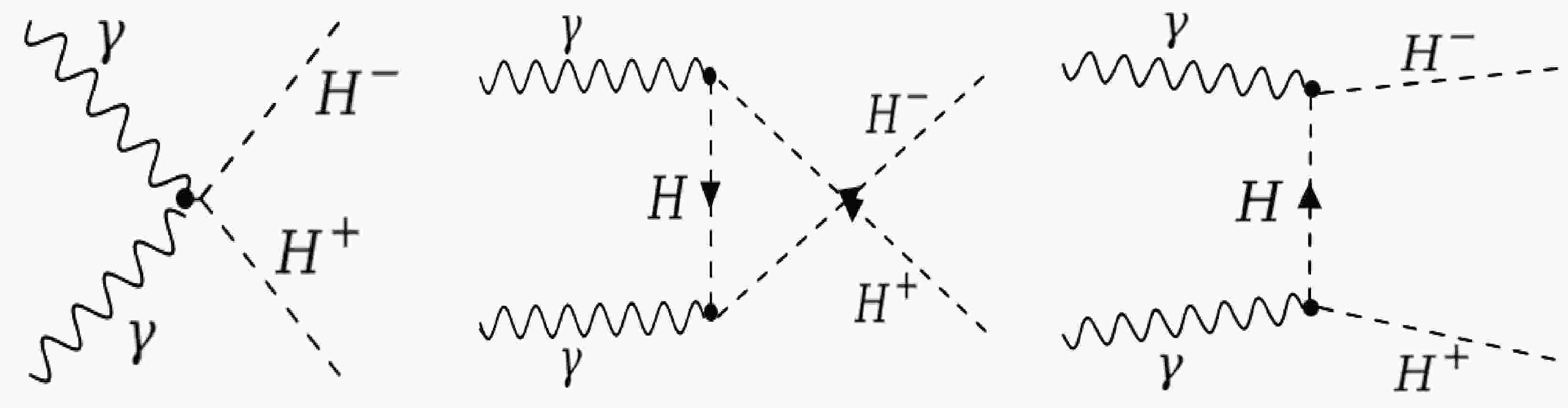
This section presents analytical formulations of the cross-section of the $ e^{+} e^{-} $ collider for the generation of a charged Higgs pair. The process used in this paper is expressed as

where $k_{a}(a=1,2,3,4)$ represents the four momenta. Three different diagrams at the tree level are topologically distinct because of photon couplings, as shown in Fig. 1. The total Feynman amplitude is given by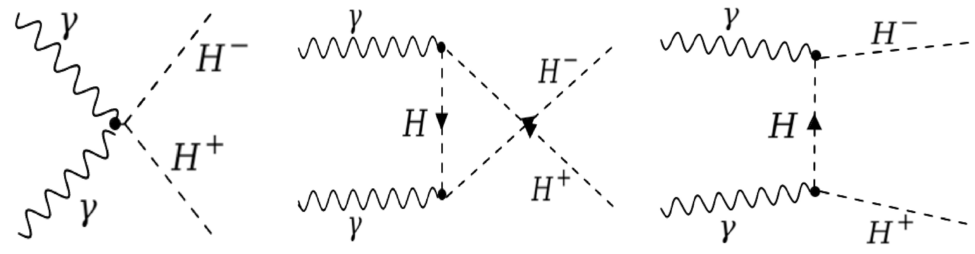

Figure 1.  Tree-level Feynman diagrams for the process $ \gamma \gamma\rightarrow H^{+}H^{-} $.

where $ \mathcal{M}_{\hat{q}},\mathcal{M}_{\hat{t}} $, and $ \mathcal{M}_{\hat{u}} $ are amplitudes of quartic couplings, t-channel, and u-channel Feynman diagrams, respectively. The relations for these channels are given as follows:

where the Mandelstam variables are represented by $ \hat{t}=(k_{1}-k_{3})^{2} $ and $ \hat{u}=(k_{2}-k_{4})^{2} $. After calculating the square of the total amplitude and summing all the foregoing matrices, we obtain the lowest order amplitude.

The scattering amplitude is calculated numerically in the center of the mass frame, where the four-momentum and scattering angle are indicated by $ (k,\theta) $. In the center of mass energy, the energy $ (k^{0}_{i}) $ and momentum $ (\overrightarrow{k}_{i}) $ of incoming and outgoing particles are

where $ m^{2}_{i} $ is the mass of relevant particles. The cross-section is calculated by taking the flux of incoming particles, and the integral over the phase space of outgoing particles is given by

In above expression, $ \lambda(s,m^{2}_{H^{+}},m^{2}_{H^{-}}) $ is the K$ \ddot{a} $llen function relevant to phase space of outgoing $ H^{\pm} $. The total integrated cross-section for the $ e^{+}e^{-} $-collider can be calculated by

where s and $ \hat{s} $ are the C.M. energies in the $ e^{+}e^{-} $-collider and subprocess of $ \gamma\gamma $, respectively. The value of $x_{\rm min}$ represents the minimum amount of energy required to generate a pair of charged Higgs particles and is given by $x_{\rm min}=(m_{H^{+}}+m_{H^{-}})/\sqrt{s}$, where $x_{\rm max}$ is 0.83 [34]. The distribution function of the photon luminosity is

The energy spectrum of Compton back-scattered photons, $ F_{\gamma/e}(x) $, is characterized by the electron beam's longitudinal momentum [34].

The numerical results of generating charged Higgs bosons via photon-photon collisions are thoroughly examined in the context of 2HDMs including QED radiations. The cross-sections at the tree level are calculated numerically for each benchmark scenario as a function of the C.M. energy and Higgs boson mass. Polarization distributions are presented to improve the production rate by considering longitudinal polarizations of initial beams. Decay pathways of the charged Higgs boson are studied for relevant scenarios.

In our work, for analytical and numerical evaluation, we have used $ \mathtt{MadGraph5\;v3.4.2} $ [35] for the calculations of the cross-sections and $ \mathtt{2HDMC\;1.8.0} $ [36] for the branching ratio and total decay width. $ \mathtt{GnuPlot} $ [37] is used for the graphical plotting.

In an electron-positron $e^-e^+ $ collider, the longitudinally polarized beam cross-section can be expressed as

In electron-positron $e^-e^+ $ colliders, beam polarization configurations are crucial for optimizing the experimental conditions and enhancing the detection of specific processes, referring to the orientation of the spins of the colliding particles, which can be manipulated to improve the signal-to-background ratio in particle interactions. Two primary types of polarization configurations are used in $e^-e^+ $ colliders: Longitudinal polarization, where both the electron and positron beams are polarized along the direction of the beam (longitudinally), either parallel or antiparallel, leading to typical configurations such as Right-Right (RR), where both beams are right-polarized, Left-Left (LL), where both beams are left-polarized, Right-Left (RL), where the electron beam is right-polarized and the positron beam is left-polarized, and Left-Right (LR), where the electron beam is left-polarized and the positron beam is right-polarized; notably, the RL and LR configurations are particularly advantageous in the context of the SM as they enhance the production rate of certain particles, such as the Higgs and Z bosons while minimizing unwanted background processes. The second configuration, transverse polarization, involves polarizing the beams perpendicular to the beam direction (not the case here), which, although less commonly used than longitudinal polarization, can provide benefits in specific scattering processes or studies of the spin structure of particles. In Fig. 2, the cross-section for the process $ \gamma\gamma\rightarrow H^{+}H^{-} $ is shown for the C.M energy of 3 TeV for three types of polarization: right handed $ RR $ ($ ++ $), oppositely-polarized $ RL $ ($ +- $), and unpolarized beam $ UU $. The cross-section is the same for the polarization modes of $ \sigma^{+-}=\sigma^{-+} $. Fig. 2 shows that the cross-section is higher for $ UU $ and $ RR $ for low $ \sqrt{s} $ and gradually decreases. However, for the $ RL $ mode of polarization, the cross-section reaches a peak value and then gradually decreases. The cross-section is not enhanced for $ RR $ and $ UU $ at higher energies but it it only for $ RL $.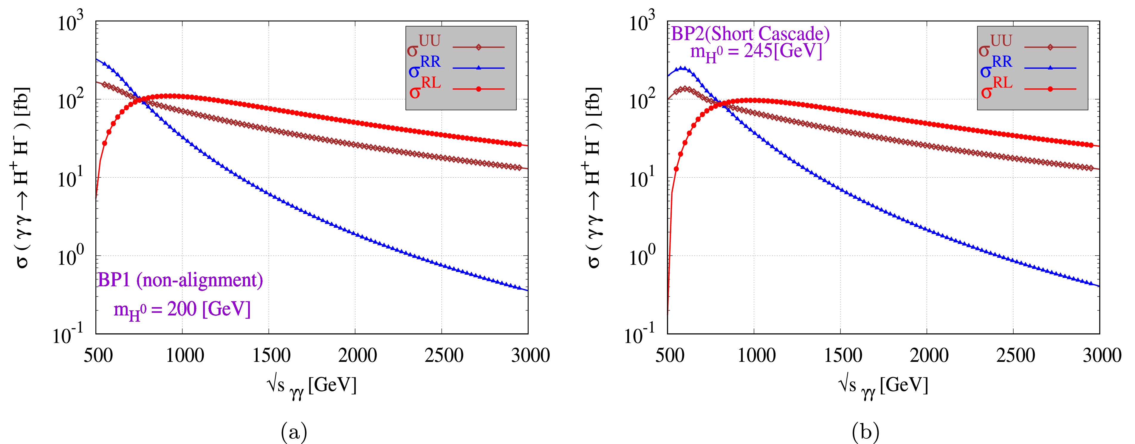

Figure 2.  (color online) Integrated cross-section for $ \gamma\gamma\rightarrow H^{+}H^{-} $ as a function of $ \sqrt{s} $ for (a) BP-1 and (b) BP-2.

In Fig. 3, for both BPs, the cross-section changes slowly with the mass of $ h^{0} $ and $ H^{0} $ because of the small range of charged Higgs mass. For both $ UU $ and $ RR $ modes of polarization, the cross-section decreases with C.M energy, and for the $ RL $ mode, it reaches a peak value and then decreases. The cross-section $ \sigma $ decreases for $ \sqrt{s} $ when $ m_{H^{\pm}}<<\sqrt{s}/2 $.

Figure 3.  (color online) Integrated cross-section for the process $ \gamma\gamma\rightarrow H^{+}H^{-} $ as a function of $ \sqrt{s} $ for (a) BP-3 and (b) BP-4.

To investigate the process in a collider, we must first identify all potentially charged Higgs products. The total decay widths of the charged Higgs boson versus the mass of $ h^{0} $ or $ H^{0} $ are plotted for all BPs. As expected, the mass of the charged Higgs boson increases with increasing neutral Higgs mass $ m_{\phi^{0}} $ under all circumstances. The decay widths are highly sensitive to the mass hierarchy and mass splitting. The decay width shrinks when $ m_{H^{0}}-m_{H^{\pm}} $, and the mass splitting is minimal, as shown in Fig. 4. The decay width for BP-1 decreases from $ 8.66 $ to $ 1.42 $ when $ m_{H^{\pm}} $ increases from $ 379 $ to $ 691\; {\rm{GeV}} $. For BP-2, the decay width increases from $ 4.38 $ to $ 5.22 $ for $ m_{H^{\pm}} $ in the range $ 250 <\; m_{H^{\pm}}\; <\; 550\; {\rm{GeV}} $. $ \Gamma_{H^{\pm}} $ for BP-3 increases from $ 3.5\times10^{-5} $ to $ 4.28 $ when $ m_{H^{\pm}} $ increases from $ 48.75 $ to $ 436\; {\rm{GeV}} $. For the last BP-4, the decay width decreases from $ 60 $ to $ 58 $ for a change in $ m_{H^{\pm}} $ from $ 558 $ to $ 564\; {\rm{GeV}} $.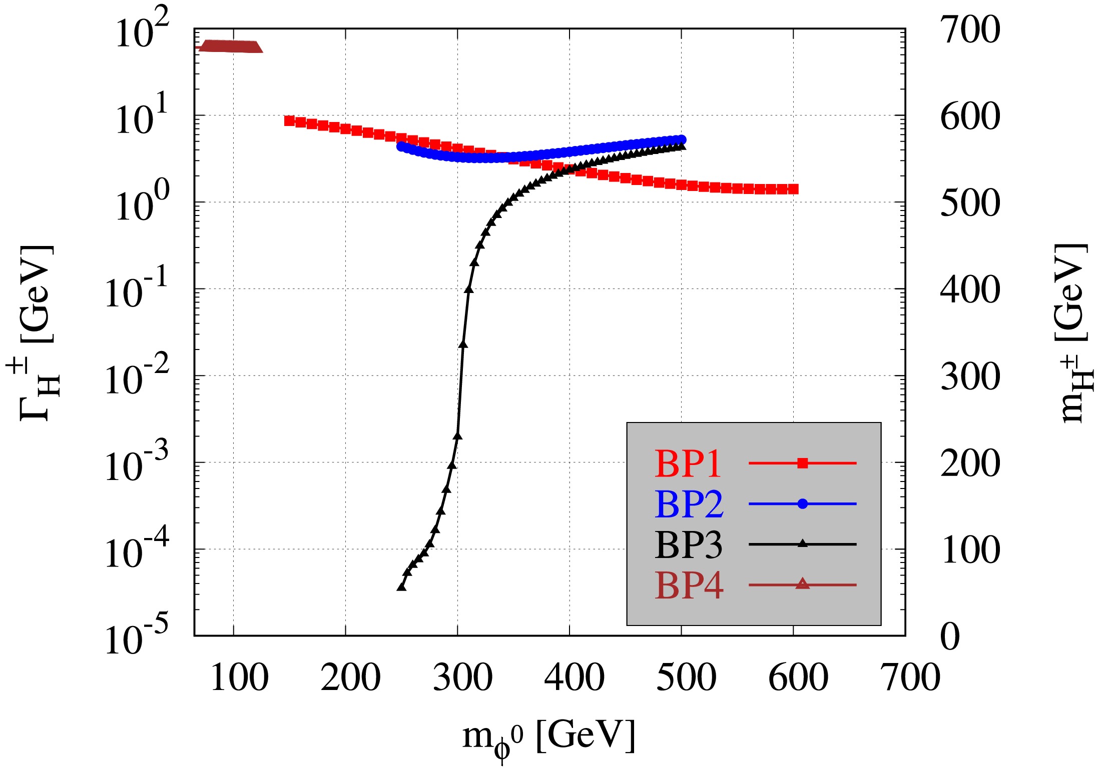

Figure 4.  (color online) Total decay widths for charged Higgs boson $ H^{\pm} $ for all benchmark points.

We show the dominant modes of BR for $ H^{\pm} $ as a function of $ h^{0} $ and $ H^{0} $ for all scenarios. The $ W^{\pm}H^{0} $ channel is the primary decay mode for $ H^{\pm} $ in BP-1, as shown in Fig. 5. The sub-dominant channels are as follows: $ t\overline {b} $ and $ W^{\pm}h^{0} $ for charged Higgs for BP-1, other suppressed channels are $ c\overline {s} $ and $ t\overline {s} $ for the range $ m_{H^{0}} < 500\; {\rm{GeV}} $. The mode of decay $ W^{\pm}h^{0} $ takes control when $BR(H^{\pm} \rightarrow W^{\pm}H^{0})$ decreases at larger values of $ m_{H^{0}} $. Therefore, for $ BR(H^{\pm} \rightarrow W^{\pm} h^{0}) $ range rises from 1.2 to 66.3% of $ 150 <m_{H^{0}}<600\; {\rm{GeV}} $. The process $ H^{0} $ to $ W^{+}W^{-} $ is another dominant decay mode with BR of 88.7% to 50.2%, and with hadronic decay of $ W^{\pm} $ has 12-jets in the final state.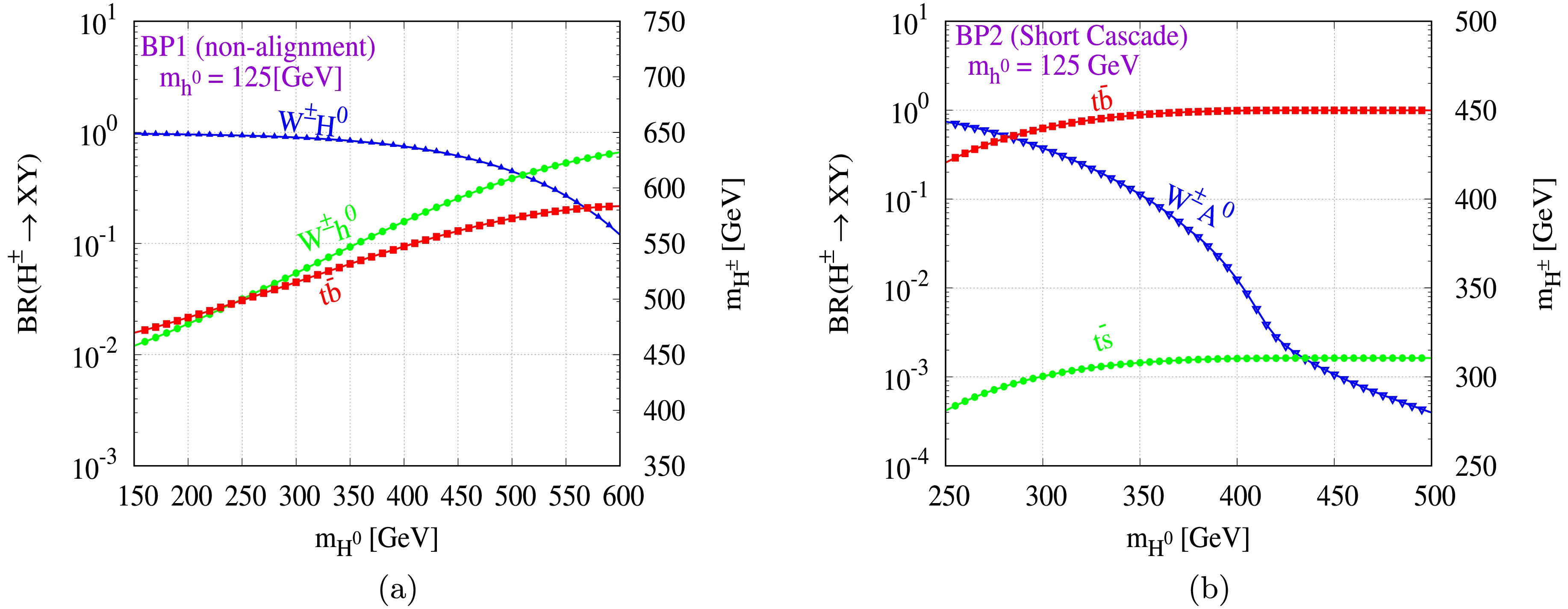

Figure 5.  (color online) BR of $ H^{\pm} $ predicted in (a) BP-1 and (b) BP-2. For modes, BR is less than $ 10^{-4} $ are omitted for clarity.

In BP-2 and BP-3, as shown in Fig. 5 and Fig. 6 respectively, as $ m_{H^{\pm}} > m_{t}+m_{b} $, the BR of 100% prominent decay mode is $ H^{\pm} \rightarrow t\overline {b} $. The suppressed decay modes of $ m_{H^{0}}<300\; {\rm{GeV}} $ are for $ W^{\pm}A^{0} $ and $ t\overline {s} $ in both BP-2 and BP-3; the $ t- $quark decay is ideal for reconstructing the process at $ m_{H^{0}}>300\; {\rm{GeV}} $. Therefore, for the process $ t\rightarrow Wb, W\rightarrow q\overline {q}(l\nu_{l}) $ gives a $ H^{\pm} $ trace at the detector, which can be tagged with 8-jets and 2-b-tagged jets. For BP-4, shown in Fig. 6, for a range of $ 65\; <m_{h^{0}}<120\; {\rm{GeV}} $, the dominant channel is $ W^{\pm}h^{0} $ because for $ \sin(\beta-\alpha)=0 $, it leads to 100%. 4-jets and 4-b-tagged jets can be used to tag the process.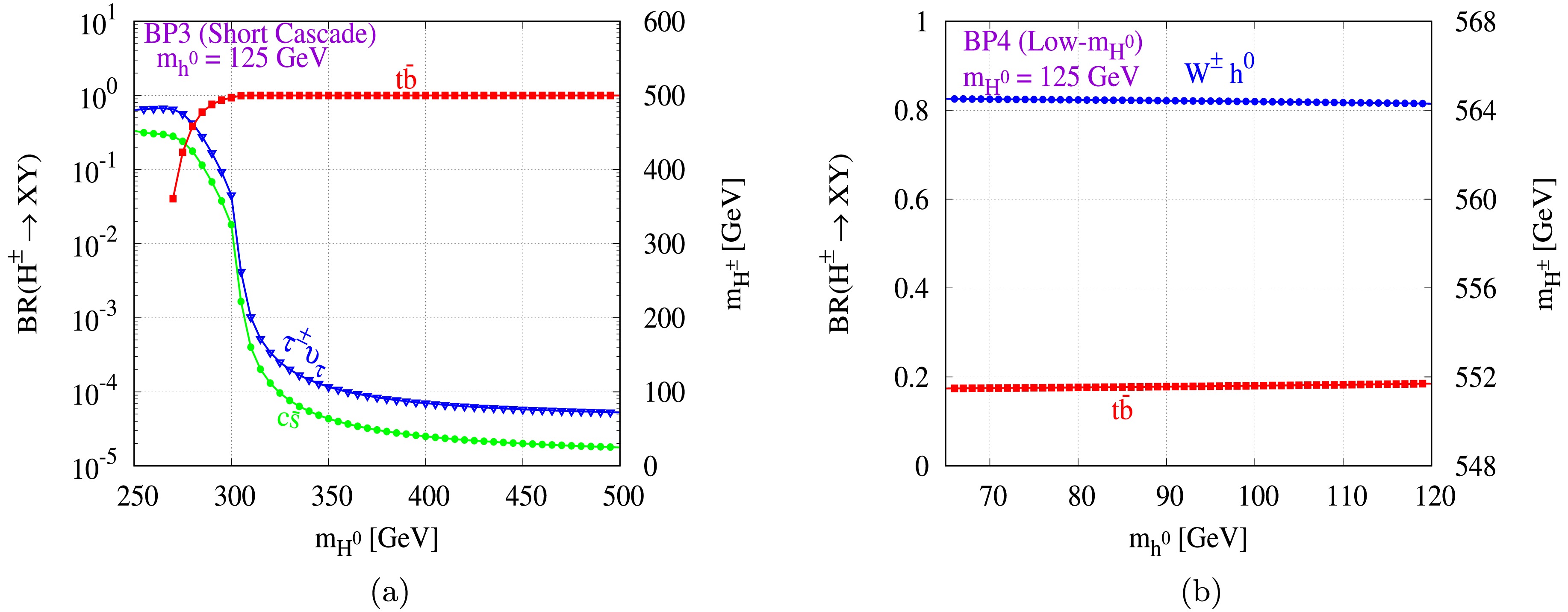

Figure 6.  BR of $ H^{\pm} $predicted in (a) BP-3 and (b) BP-4. For all modes, BR is less than$ 10^{-4} $ are omitted for clarity.

An integrated ROOT framework for parallel running and computation of several multivariate categorization algorithms is called the “Toolkit for Multivariate Analysis” (TMVA) [38], which categorizes using two sorts of events: signal and background. TMVA has many applications in high energy physics for the complex multiparticle final state. To train the classifiers, a set of events with well-defined event types is inserted into the Factory. The event samples for signal and background can either be read using a tree-like structure or a plain text file using a defined structure. All variables that must have separate signal and background events must be known by the Factory. Cuts are applied on signal and background trees separately.

We present three classifiers in our work: Boosted Decision Tree (BDT), LikelihoodD (Decorrelation), and Multilayer Perceptron (MLP). In BDT, a selection Tree is a tree-like structure that illustrates the different outcomes of a choice using a branching mechanism. An event is categorized as either a signal or background event by passing or failing to pass a condition (cut) on a certain node until a choice is reached. The ''root node'' of the decision tree is used to determine these cuts. The node-splitting process concludes when the BDT algorithm specifies minimal events ($ \mathtt{NEventsMin} $). The final nodes (leaves) are classified according to their ''purity'' (p). The value for signal or background (typically $ +1 $ for the signal and 0 or $ -1 $ for the background) depends on whether p is greater than or less than the stated number, e.g., +1 if $ p>0.5 $ and $ -1 $ if $ p<0.5 $ [39]. To differentiate between the background class and signal, we conduct a labeling process. All occurrences with a classifier output$y > y_{\rm cut}$ are labeled as a signal, whereas the remainder are classified as background. The purity of the signal efficiency $\epsilon_{\rm sig, eff}$ and background rejection ($1- \epsilon_{\rm bkg, eff}$) are evaluated for each cut value of $y_{\rm cut}$ [40]. The ADA-Boost algorithm re-weights every misclassified event candidate. The new candidate weight consists of the one used in the former tree multiplied by $ \alpha=1-\Delta_{m}/\Delta_{m} $, where $ \Delta_{m} $ is the misclassification error. This leads to an increase in the weight and therefore an increase in the candidate’s importance when searching for the best separation values. The weights of each new tree are based on the ones of its predecessors [41]. An Artificial Neural Network (ANN) comprises linked neurons, each with its weight. To accelerate the processing, we can use a reduced layout as well, the so-called MLP. The network consists of three types of layers: the input layer, consisting of$ n_{var} $ neurons and a bias neuron, many deep layers containing a user-specified number of neurons (set in the option $ \mathtt{HiddenLayers} $) plus a bias node, and an output layer; each of the connections between two neurons carries a weight.

For event j, the likelihood ratio $ y_{L} (j) $ is defined by

where the likelihood of a candidate to be signal/background may be determined using the following formula:

where $ P_{S/B, i} $ is the PDF for the ith input variable $ x_{i} $. The PDFs are normalized to 1 for all i:

The projective likelihood classifier has a major limitation in that it does not use correlation among the discriminating input variables. In the realistic approach, it does not provide an accurate analysis and leads to performance loss. Even other classifiers underperform in the presence of variable correlation. Linear Correlation is used to quantify the training sample by obtaining the square root of the covariant matrix. The square root of the matrix C is $ C^{'} $, which when multiplied by itself yields $ C: C=(C^{'})^{2} $. As a result, TMVA employs diagonalization of the (symmetric) covariance matrix provided by

D is the diagonal matrix, and S denotes the symmetric matrix. The linear decorrelation is calculated by multiplying the starting variable x by the inverse of $ C^{'} $.

Only linearly coupled and Gaussian distributed variables have a full decorrelation. In this work, the signal and background events are taken to be 50000 with applied cuts:

The curve of background rejection against signal efficiency provides a reasonable estimate of a classifier’s performance. A classifier’s performance is measured by the area under the signal efficiency versus the background rejection curve. Therefore, the larger the area, the better a classifier’s predicted separation power, as shown in Fig. 7. The values of area under the curve (AUC) for Fig. 7 are shown in Table 4. The table shows that the best classifier among all is the MLP and BDT, improved after applying cuts, and provided the largest AUC. We used 800 trees to improve the BDT’s performance, with node splitting at the 2.5% event threshold. The max tree depth was set at 3. We performed training using Adaptive Boost with a learning rate of $ \beta = 0.5 $. The parent node and sum of the indices of the two daughter nodes were compared to optimize the cut value on the variable in a node. For the separation index, we use the Gini Index. Finally, the variable’s range was evenly graded into 20 cells. The signal values were taken as 1 and background values approach 0.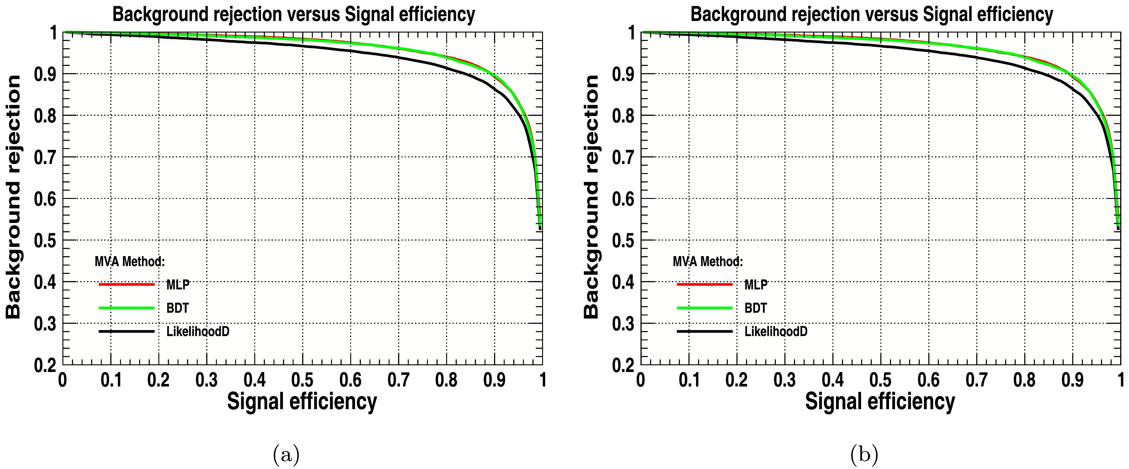

Figure 7.  (color online) Background Rejection vs Signal Efficiency (a) with cuts and (b) without cuts.

Figs. 8, 9, and 10 have been specifically generated for BP1 at a center-of-mass energy of $ \sqrt{s} $ = 3 TeV and 3000 ${\rm{fb}}^{-1}$, ensuring that the results accurately reflect the expected physical behaviors and interactions at this energy scale under the defined experimental conditions. Figure 8 depicts that the signal significance, $ S/\sqrt{S+B} $, of the classifier is improved by applying cuts with an optimal cut of -0.0271. Similarly, Fig. 9 shows the best classifier that is improved by applying cuts with an optimal cut value of 0.1741, and the signal efficiency is also higher than without applied cuts. The LikelihoodD signal significance is shown in Fig. 10, which has been improved by applied cuts with an optimal cut of 0.0501.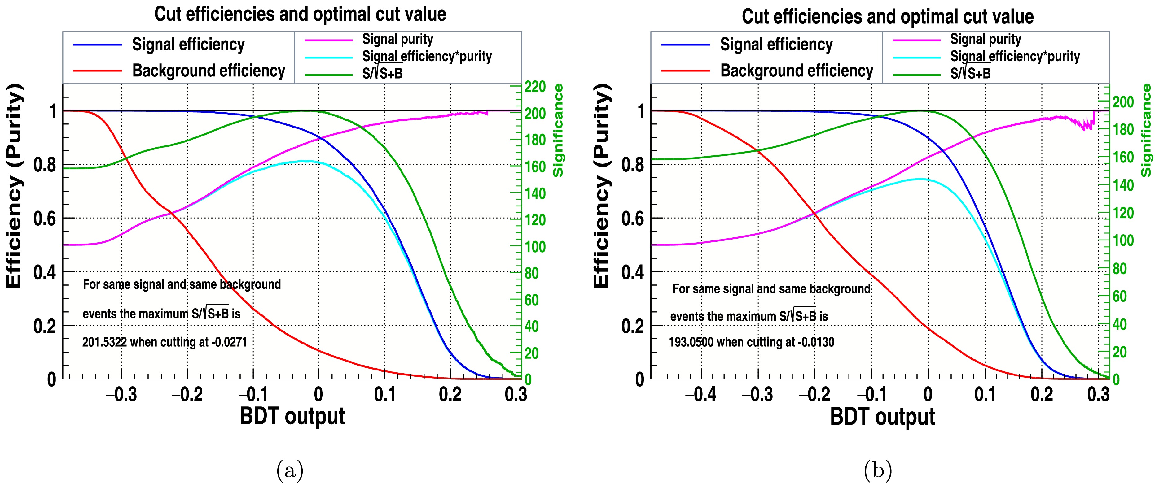

Figure 8.  (color online) BDT signal significance (a) with cuts and (b) without cuts.

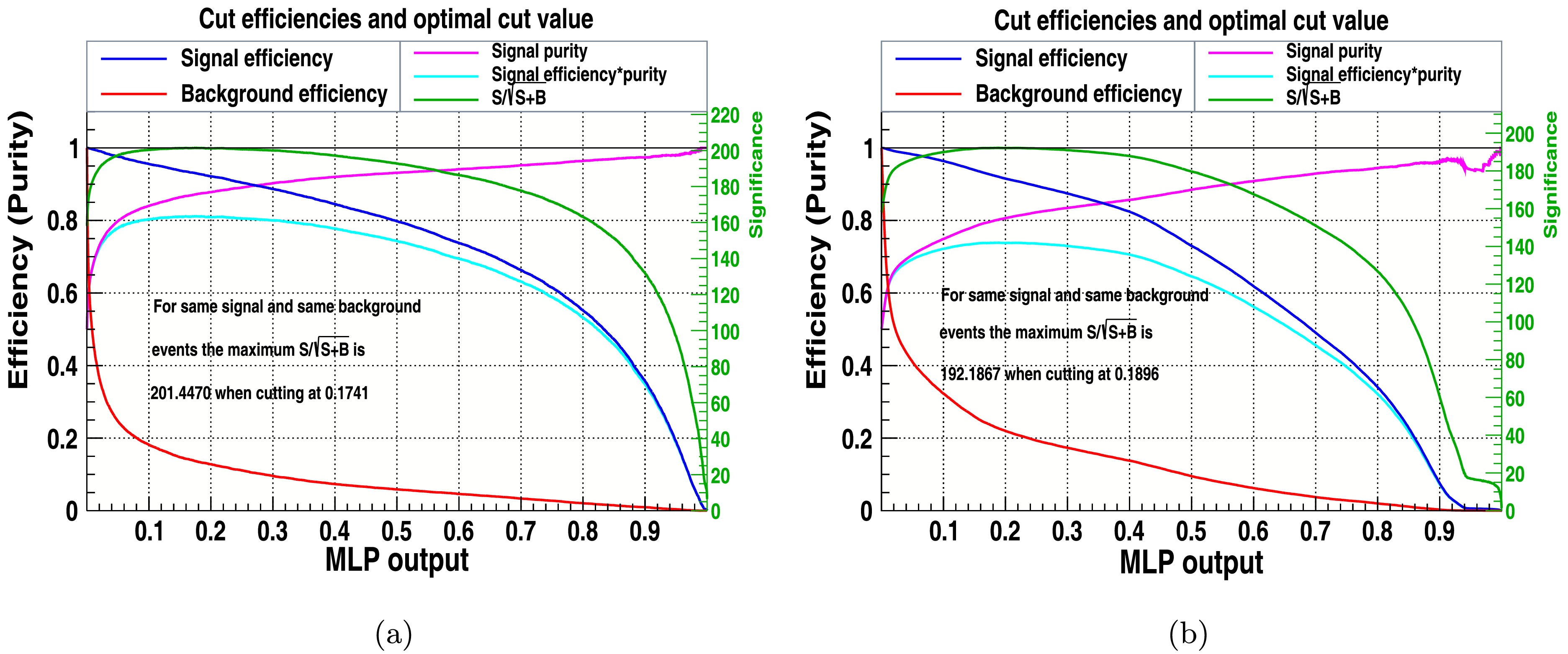
Figure 9.  (color online) MLP Signal Significance (a) with cuts and (b) without cuts.

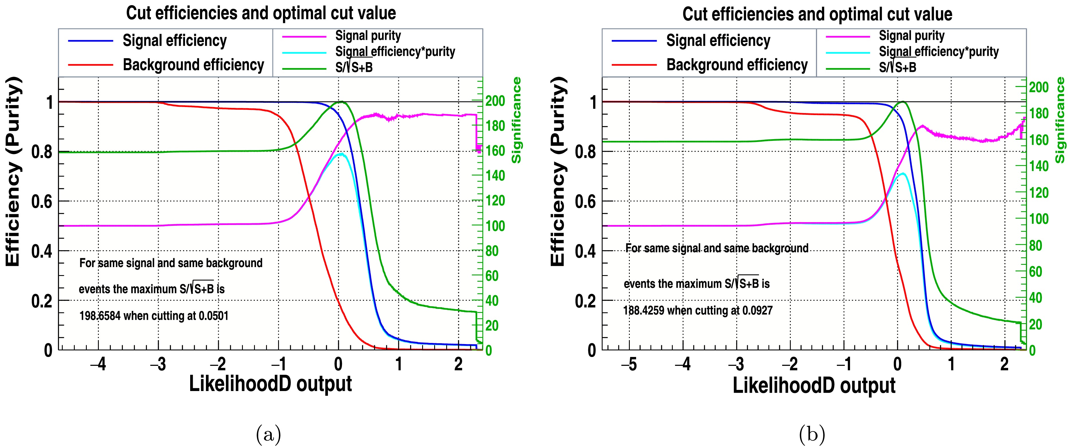
Figure 10.  (color online) LikelihoodD Signal Significance (a) with cuts and (b) without cuts.

The simplest extension of the SM is the 2HDM containing a charged Higgs boson, and the exact measurement of its nature and corresponding model parameters are crucial for its discovery. The pair production is one of the best channels that provide the observable signal in the vast range of parameters in 2HDM.

The generation rates of incoming beams are investigated under various polarization collision patterns. The cross-section can be increased twice by oppositely polarized beams of photons at high energies and right-handed polarized beams of photons at low energies as shown in the figures of the cross-section. For BP-1, at $\sqrt{s}=3\; {\rm TeV}$, $\sigma^{UU}=12.92\pm 8.1 \times 10^{-6}$ fb, $\sigma^{RR}=0.3568 \pm 4.6 \times 10^{-7}$fb, and$\sigma^{RL}=25.48 \pm 1.6 \times 10^{-5}$ fb. For BP-2, the cross-section for $\sigma^{UU}=12.76 \pm 8.03 \times 10^{-6}$ fb, $\sigma^{RR}=0.4067 \pm 5.3 \times 10^{-7}$fb, and $\sigma^{RL}=25.11 \pm 1.8 \times 10^{-5}$ fb at the center of mass energy of $3\; {\rm TeV}$. The cross-section at $3\; {\rm TeV}$ for BP-3 for different polarizations is $\sigma^{UU}=13.22 \pm 9.1 \times 10^{-6}$ fb, $\sigma^{RR}=0.2674 \pm 3.2 \times 10^{-7}$ fb, and $\sigma^{RL}=26.17 \pm 1.7 \times 10^{-5}$ fb. In the low-$ m_{H} $ scenario for BP-4, the cross-sections for polarized beams is $\sigma^{UU}=13.23 \pm $$9.1 \times 10^{-6}$ fb, $\sigma^{RR}=0.2673 \pm 3.2 \times 10^{-7}$ fb, and $\sigma^{RL}=26.19 \pm 1.7 \times 10^{-5}$ fb at $ \sqrt{s}=3\; {\rm{TeV}} $. Therefore, we conclude that for all BPs, the cross-section is low at a high energy for $ UU $ and $ RR $ polarized beams of photons and high for $ RL $ at a high energy.

For each scenario, the reconstruction of the charged Higgs Boson has been provided, and its prominent decay modes have been examined. The branching ratio of the decay channel for non-alignment, the bosonic decay channel $ H^{\pm}\rightarrow W^{\pm}H^{0} $ is dominant, whereas in the low$ -m_{H} $ scenarios, the bosonic decay of $ W^{\pm}h^{0} $ is dominant, increasing to 66.3%. The 100% dominant decay channel in a short-cascade scenario is $ H^{\pm}\rightarrow t \bar{b} $, which indicates that the t decay is the ideal candidate for the reconstruction of the process. Limited phase space and alignment constraints restrict bosonic decay channels.

Our machine-learning models for multivariate analysis results are improved by applying cuts. The signal efficiency $(\epsilon_{\rm Sig, eff})$ and background rejection $(1-\epsilon_{\rm Bkg, eff})$ are increased when cuts are applied to the MLP, BDT, and LikelihoodD classifiers. The AUCs for MLP, BDT, and LikelihoodD increase to 3.9%, 3.46%, and 5.02%, respectively. This shows that LikelihoodD is the more efficient classifier for signal efficiency and background rejection. The signal significance for MLP, BDT, and LikelihoodD increase to 4.81%, 4.39%, and 5.43%, respectively, when cuts are applied. The significance values obtained with cuts demonstrate how well these models can separate charged Higgs production-related background events from signal occurrences. These cuts most likely aid in lowering background noise, enhancing overall performance, and separating signal events associated with charged Higgs generation. This consistency upholds the validity of the selected machine-learning approaches and increases trust in the outcomes.