


 Abstract
 HTML
HTML Reference
 Related
 PDF
PDF


-
Following the discovery of the Higgs boson at the Large Hadron Collider (LHC) [1, 2], precise measurements of its properties, including mass, spin, and couplings to gauge bosons and fermions, became critically important [3−9]. To date, these measurements have been consistent with the expectations of the Standard Model (SM) [10, 11]. However, the trilinear and quartic Higgs self-couplings, denoted as
$ \lambda_{{\rm{3H}}} $ and$ \lambda_{{\rm{4H}}} $ , respectively, which represent a fundamental aspect of the SM that connects the Higgs mechanism and the stability of our Universe [12], are still subject to large uncertainties.Significant efforts have been dedicated to improving the measurement of the Higgs self-coupling. The most direct approach involves measuring the cross section of Higgs boson pair production, predominantly through gluon-gluon fusion (ggF). At the leading order (LO), this process occurs via a top-quark loop. In the large top-quark mass (
$ m_t $ ) limit, the cross section of ggF Higgs boson pair production is known up to next-to-next-to-next-to-leading-order (N$ ^{3} $ LO) QCD corrections [13−17], with the calculation of the soft gluon resummation effect also being studied [18−20]. When considering the full$ m_t $ dependence, only next-to-leading-order (NLO) QCD corrections are available [21−24], while estimates of the finite$ m_t $ effects at next-to-next-to-leading-order (NNLO) have been conducted [25−29]. A comprehensive simulation of events necessitates a fully differential calculation of the Higgs boson pair production and decay to the$ b\bar{b}\gamma\gamma $ final state at QCD NLO [30]. Furthermore, NLO electroweak corrections have been explored [31−37]. The subdominant channel—vector boson fusion (VBF)—has also been computed up to N3LO in QCD [38−42].The current constraints on the trilinear Higgs self-coupling extracted from the Run 2 dataset of Higgs boson pair production at the LHC by the ATLAS and CMS collaborations are
$ -0.6<\kappa_{\lambda_{{\rm{3H}}}}<6.6 $ [43] and$-1.24 < \kappa_{\lambda_{{\rm{3H}}}}<$ 6.49 [11], respectively, within the$ \kappa $ framework [44], where$ \kappa_{\lambda_{{\rm{3H}}}}=\lambda_{{\rm{3H}}}/\lambda_{{\rm{3H}}}^{{\rm{SM}}} $ , with$ \lambda_{{\rm{3H}}}^{{\rm{SM}}} $ being the SM value of the trilinear Higgs self-coupling. Meanwhile, the process of single Higgs boson production and decay depends on the Higgs self-coupling only via higher-order electro-weak (EW) corrections and can also impose certain constraints [45−50]. Measurement based on the differential fiducial cross section in bins of the Higgs boson transverse momentum sets a constraint of$ -5.4<\kappa_{\lambda_{{\rm{3H}}}}< $ 14.9 [51]. Combined analyses of single- and double-Higgs production result in the constraint$ -0.4<\kappa_{\lambda_{{\rm{3H}}}}< $ 6.3 at the 95% confidence level, assuming that new physics changes only the Higgs self-coupling [43].These constraints stem from considering the cross section of Higgs boson pair production as a function of the Higgs self-coupling. Indeed, even with higher-order QCD corrections, the cross section is a quadratic function of the trilinear Higgs self-coupling,
$ \lambda_{{\rm{3H}}} $ . Nevertheless, higher-order EW corrections introduce contributions from Feynman diagrams containing one or more triple Higgs or quadruple Higgs vertices, leading to a distinct functional dependence on the Higgs self-coupling. Specifically, new quartic and cubic power dependencies on the trilinear Higgs self-coupling emerge, which has a significant impact on the constraints, given that the current upper limit is notably large.In practical calculations, maintaining an explicit dependence on the Higgs self-coupling can be challenging given that it is typically treated as a derived parameter in the conventional calculation of EW corrections, particularly during the renormalization process [35, 52]. Even if one can perform the renormalization by taking the Higgs self-coupling as a primary parameter, it is not clear how the relation
$ m_H^2=2\lambda v^2 $ can be implemented and the Higgs self-coupling can be rescaled. Different choices lead to different expressions for the cross sections. Therefore, the calculation of the EW corrections in the SM cannot be extended to the case with general$ \lambda_{{\rm{3H}}} $ and$ \lambda_{{\rm{4H}}} $ , and the cross section with higher power (beyond quadratic) dependence on the Higgs self-couplings in the general$ \kappa $ framework is still lacking.To address this challenge, we propose a renormalization procedure that explicitly retains the Higgs self-couplings at each step and introduce renormalization of the coupling modifier. By combining this procedure with analytical and numerical calculations of the complex one-loop and two-loop amplitudes, respectively, we derive the cross sections of the Higgs boson pair production in both the ggF and VBF channels as functions of the Higgs self-couplings. Our findings indicate that incorporating higher power dependencies of the cross section on the Higgs self-couplings can reduce the upper limit of
$ \kappa_{\lambda_{{\rm{3H}}}} $ by approximately 20%. -
The LO contribution to the ggF Higgs boson pair production
$ g(p_1)g(p_2)\to H(p_3)H(p_4) $ arises from the top-quark induced triangle and box Feynman diagrams, which are of order$ \lambda_{{\rm{3H}}} $ and$ \lambda_{{\rm{3H}}}^0 $ , respectively. Therefore, the LO cross section at the 13 TeV LHC can be expressed as$ \begin{aligned} \sigma_{{\rm{ggF,LO}}}^{\kappa_{\lambda}}=(\; 4.72\; \kappa_{\lambda_{{\rm{3H}}}}^2-23.0\; \kappa_{\lambda_{{\rm{3H}}}}+35.0 \; )\; \; {{\rm{fb}}}. \end{aligned} $

(1) Here, the subscript
$ \lambda_{{\rm{3H}}} $ in$ \kappa_{\lambda_{{\rm{3H}}}} $ signifies the deviation of the trilinear Higgs self-coupling from its SM value. Below, we also introduce$ \kappa_{\lambda_{{\rm{4H}}}} $ to denote the modification of the quartic Higgs self-coupling. The SM cross section is recovered when$ \kappa_{\lambda_{{\rm{3H}}}}=1 $ and$ \kappa_{\lambda_{{\rm{4H}}}}=1 $ . This quadratic functional form persists even with the inclusion of higher-order QCD corrections [53], e.g.,$ \begin{aligned} \sigma_{{\rm{ggF, NNLO-FT}}}^{\kappa_{\lambda}}=(\; 10.8\; \kappa_{\lambda_{{\rm{3H}}}}^2-49.6\; \kappa_{\lambda_{{\rm{3H}}}}+ 70.0\; )\; \; {{\rm{fb}}}. \end{aligned} $

(2) In this expression, the full one-loop real contributions are merged with other NNLO QCD corrections in the large
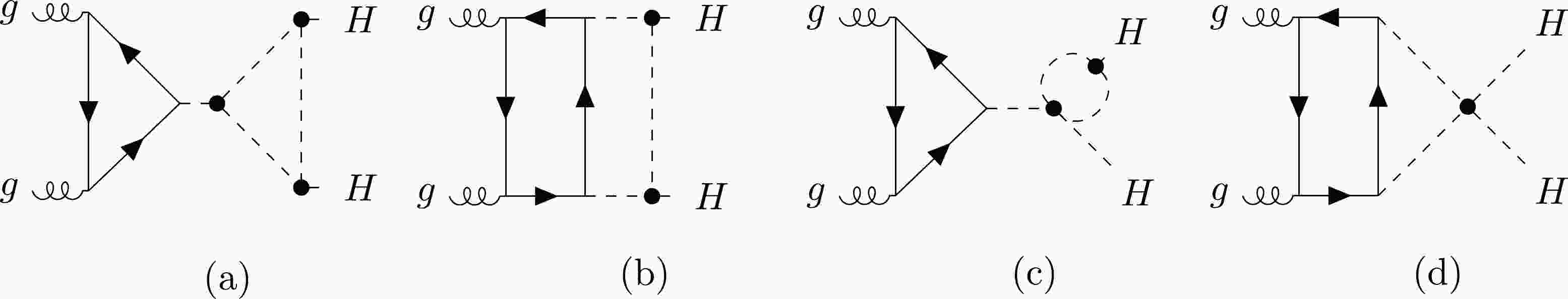
$ m_t $ limit. It is worth noting that the effects of QCD corrections are substantial, with each term in$ \kappa_{\lambda_{{\rm{3H}}}} $ more than doubling in value compared to the LO expression.The EW corrections change the above functional form in two aspects. First, the coefficients of the quadratic, linear, and constant terms are altered by the corrections induced by virtual gauge bosons. However, the overall impact is relatively minor, typically amounting to only a few percent, as reported in Ref. [35]. Given this negligible influence on the constraints related to the Higgs self-coupling, these corrections are deemed insignificant for the purposes of our study and are consequently omitted. Second, higher power or new dependence on the Higgs self-couplings arises from the corrections induced by virtual Higgs bosons. Fig. 1 shows some typical two-loop Feynman diagrams, which give contributions of order
$ \lambda_{{\rm{3H}}}^3 $ ,$ \lambda_{{\rm{3H}}}^2 $ ,$ \lambda_{{\rm{4H}}} \lambda_{{\rm{3H}}} $ ,$ \lambda_{{\rm{4H}}} $ to the amplitudes. As a result, the cross section contains new quartic and cubic powers of$ \lambda_{{\rm{3H}}} $ and starts to be sensitive to the quartic Higgs self-coupling$ \lambda_{{\rm{4H}}} $ . Our objective is to assess these corrections, denoted by$ \delta \sigma_{{\rm{EW}}}^{\kappa_\lambda} $ , and their impact on the constraints on the Higgs self-couplings.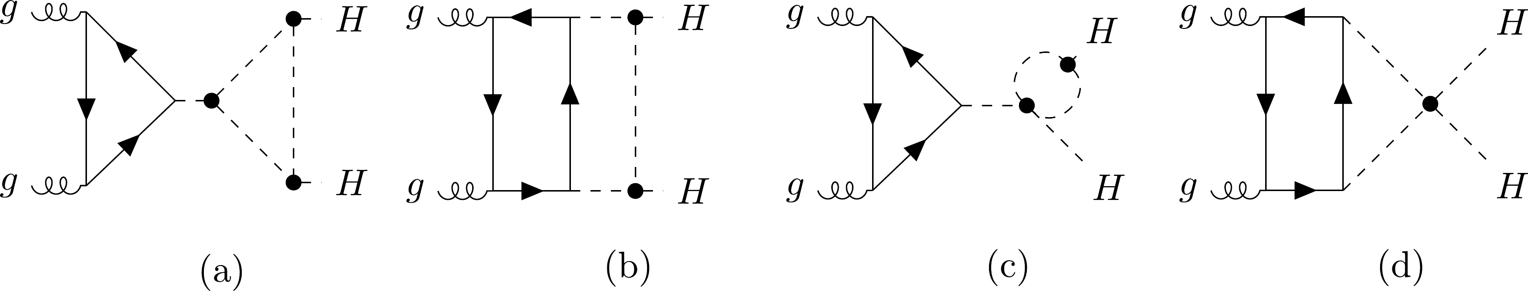
Figure 1. Typical two-loop Feynman diagrams of order
$\lambda^3_{{\rm{3H}}}~(a), \lambda^2_{{\rm{3H}}}~(b), \lambda_{{\rm{4H}}} \lambda_{{\rm{3H}}} ~(c)$ , and$\lambda_{{\rm{4H}}}~(d) $ , respectively.Our calculations for two-loop diagrams were realized as follows. We used FeynArts [54] to generate the Feynman diagrams and corresponding amplitudes. The amplitudes were expressed as a linear combination of two tensor structures with the coefficients called form factors [55]. After performing the Dirac algebra with FeynCalc [56−58], we obtained scalar integrals for each form factor. Rather than reducing all scalar integrals to master integrals and establishing differential equations for these master integrals, we directly computed the scalar integrals for specific phase space points employing the numerical package AMFlow [59, 60]. This decision was motivated by the intricate nature of constructing differential equations, particularly with general kinematic dependencies, which can be exceedingly time-consuming. Even if the differential equation is derived, obtaining an analytical solution appears infeasible with current technologies owing to the presence of massive propagators. Numerical solutions of these differential equations often suffer from accuracy loss. By contrast, direct numerical calculation at each phase space point ensures accuracy. The primary challenge lies in covering the entire phase space efficiently. Fortunately, the process of
$ gg\to HH $ is dominated by S-wave scattering, making the amplitude insensitive to the scattering angle. Moreover, its dependence on the scattering energy is also weak, except in very high-energy regions, as shown below. These characteristics enable the generation of a grid with a limited data set. This grid can be used to accurately calculate the amplitude at any point in the phase space.Note that the sum of all one-particle irreducible two-loop diagrams is finite. However, the sum of one-particle reducible two-loop diagrams contains ultraviolet divergences. They will cancel after considering the contributions from the counter-terms in renormalization.
In the SM, the Lagrangian for the Higgs sector can be expressed as
$ \begin{aligned} \mathcal{L}_{{\rm{H}}}=(D_{\mu}\phi_0)^{\dagger}(D^{\mu}\phi_0)+\mu_0^2(\phi_0^{\dagger}\phi_0)-\lambda_0(\phi_0^{\dagger}\phi_0)^2, \end{aligned} $

(3) where
$ \phi_0 $ denotes the bare Higgs doublet and$ D_{\mu} $ is the covariant derivative. The relations between the bare quantities and their renormalized counterparts are given by$ \phi_0 = Z^{1/2}_{\phi}\phi\,, \mu^2_0 = Z_{\mu^2}\mu^2\,, $ and$ \lambda_0 = Z_{\lambda}\lambda. $ The EW gauge symmetry is spontaneously broken once the Higgs field develops a non-vanishing vacuum expectation value
$ v $ . Taking the unitary gauge, we can express the Higgs field as$ \begin{aligned} \phi=\frac{1}{\sqrt{2}} \left( \begin{array}{c} 0 \\ H + Z_v v \end{array} \right), \end{aligned} $

(4) where
$ Z_v $ is the renormalization constant for the vacuum expectation value. The renormalized Lagrangian in the$ \kappa $ framework after EW gauge symmetry breaking is given by$ \begin{aligned}[b] \mathcal{L}_{{\rm{H}}}^{\kappa}=\;&\frac{1}{2}Z_{\phi}(\partial_{\mu}H)^2-\left(-\frac{1}{2}Z_{\mu^2}Z_{\phi}Z_v^2 \mu^2 v^2+\frac{1}{4}Z_{\lambda}Z_{\phi}^2 Z_v^4 \lambda v^4\right) \\&-(Z_{\lambda}Z_{\phi}^2 Z_v^3 \lambda v^3-Z_{\mu^2}Z_{\phi} Z_v \mu^2 v)H \\ &-\left(\frac{3}{2}Z_{\lambda}Z_{\phi}^2 Z_v^2 \lambda v^2-\frac{1}{2}Z_{\mu^2}Z_{\phi}\mu^2\right)H^2 -Z_{\kappa_{{\rm{3H}}} } Z_{\lambda}Z_{\phi}^2 Z_v \lambda_{{\rm{3H}}} v H^3 \\&-\frac{1}{4}Z_{\kappa_{{\rm{4H}}} } Z_{\lambda}Z_{\phi}^2\lambda_{{\rm{4H}}} H^4+\cdots\,, \end{aligned} $

(5) where the ellipsis represents the terms involving EW gauge bosons. Note that the letter
$ \lambda $ is solely used for the Higgs self-coupling in the SM but$ \lambda_{{\rm{3H}}}\equiv \kappa_{\lambda_{{\rm{3H}}}}\lambda $ and$ \lambda_{{\rm{4H}}}\equiv \kappa_{\lambda_{{\rm{4H}}}}\lambda $ denote the Higgs self-couplings that could be modified by new physics. We have added the renormalization constants$ Z_{\kappa_{{\rm{3H}}} } $ and$ Z_{\kappa_{{\rm{4H}}} } $ for the coupling modifiers$ \kappa_{\lambda_{{\rm{3H}}}} $ and$ \kappa_{\lambda_{{\rm{4H}}}} $ to account for potential new physics effect in renormalization. Following the general principle of the$ \kappa $ framework, we have assumed that the new physics does not affect the vacuum expectation value and Higgs mass when we rescale the Higgs self-couplings. The second term in the first line of Eq. (5) contains no field and thus can be safely dropped. Writing$ Z=1+\delta Z $ , the third term can be expanded as$ \begin{aligned}[b]& (\mu^2 v - \lambda v^3)H + [ (\delta Z_{\mu^2}+\delta Z_{\phi}+\delta Z_v)\mu^2 v \\&\quad- ( \delta Z_{\lambda} + 2\delta Z_{\phi}+3\delta Z_v ) \lambda v^3 ]H +\cdots \end{aligned} $

(6) where we have neglected higher-order corrections that are products of two
$ \delta Z $ 's. The renormalization condition is set such that there is no tadpole contribution. This condition requires$ \mu^2 = \lambda v^2 $ at the tree level and$(\delta Z_{\mu^2}-\delta Z_{\lambda}- \delta Z_{\phi} -2\delta Z_v )\mu^2 v + T =0$ at the one-loop level, with$ T $ being the contribution from the one-loop tadpole diagrams. The vacuum expectation value appears always in the form of$ Z_{\phi}^{1/2}Z_v v $ and is closely related to the massive gauge boson mass. Therefore,$ \delta Z_v $ would be determined only after considering the renormalization of the EW gauge sector. Given that we focus on the corrections induced by the Higgs self-couplings, we can simply take$ \delta Z_v + \delta Z_{\phi}/2 = 0 $ . We adopt dimensional regularization, i.e., the space-time dimension is set as$ d=4-2\epsilon $ to regulate the ultraviolet divergence, and$ \mu_R $ is selected as the renormalization scale. The tadpole diagram is evaluated to be$ \begin{aligned} T = \frac{3 \lambda_{{\rm{3H}}} v}{16\pi^2}m_H^2\left(\frac{1}{\epsilon}+\ln\frac{\mu_R^2}{m_H^2}+1\right)\,. \end{aligned} $

(7) The mass of the Higgs boson,
$ m_H $ , can be determined from the quadratic term in Eq. (5) as follows:$ \begin{aligned}[b] & \frac{1}{2}(\partial_{\mu}H)^2 -\mu^2 H^2+\frac{1}{2}\delta Z_{\phi} (\partial_{\mu}H)^2 \\&- \left(\frac{3}{2}\delta Z_{\lambda}+\frac{5}{2}\delta Z_{\phi} -\frac{1}{2}\delta Z_{\mu^2} + 3\delta Z_v \right)\mu^2 H^2 \\ \equiv \;& \frac{1}{2}(\partial_{\mu}H)^2 -\frac{1}{2}m_H^2 H^2 +\frac{1}{2}\delta Z_{\phi} (\partial_{\mu}H)^2 \\&- \frac{1}{2}(\delta Z_{m_H^2} + \delta Z_{\phi} ) m_H^2 H^2 \,. \end{aligned} $

(8) On the right-hand side, we have introduced the classical mass terms. By comparing both sides, it is straightforward to obtain that
$ m_H^2 = 2\mu^2 $ and$ \delta Z_{m_H^2} \equiv \frac{3}{2}\delta Z_{\lambda}+\frac{3}{2}\delta Z_{\phi} - \frac{1}{2}\delta Z_{\mu^2} + 3\delta Z_v $ . Applying the on-shell renormalization condition for the Higgs field, we obtain$ \begin{aligned}[b] \delta Z_{m_H^2} =\;&\frac{3\lambda_{{\rm{4H}}}}{16\pi^2}\left(\frac{1}{\epsilon}+\ln\frac{\mu^2_R}{m_H^2}+1\right) \\&+\frac{9\lambda_{{\rm{3H}}}^2 v^2}{m_H^2}\frac{1}{8\pi^2}\left(\frac{1}{\epsilon}+\ln\frac{\mu^2_R}{m_H^2}+2-\frac{\pi}{\sqrt{3}}\right), \\ \delta Z_{\phi} =\;&\frac{9\lambda_{{\rm{3H}}}^2 v^2}{8\pi^2}\frac{\sqrt{3}-2\pi/3}{\sqrt{3}m_H^2}\,. \end{aligned} $

(9) Combining the above equations, we derive results for the other renormalization constants, namely
$ \delta Z_{\mu^2} $ and$ \delta Z_{\lambda} $ . Then, the counter-term for the triple Higgs interaction in Eq. (5) is given by$ \begin{aligned}[b] \delta \lambda_{{\rm{3H}}} \equiv\;& \delta Z_{\lambda} + 2\delta Z_{\phi}+\delta Z_{v} +\delta Z_{\kappa_{{\rm{3H}}} } \\ =\;&-\frac{3\lambda_{{\rm{3H}}}}{16\pi^2}\left(\frac{1}{\epsilon}+\ln\frac{\mu_R^2}{m_H^2}+1\right)+ \frac{3\lambda_{{\rm{4H}}}}{16\pi^2}\left(\frac{1}{\epsilon}+\ln\frac{\mu_R^2}{m_H^2}+1\right) \\ & +\frac{3\lambda_{{\rm{3H}}}^2 v^2}{16\pi^2m_H^2}\left(\frac{6}{\epsilon}+6\ln\frac{\mu_R^2}{m_H^2}+21-4\sqrt{3}\pi\right) +\delta Z_{\kappa_{3H} } \end{aligned} $

(10) with
$ \delta Z_{\kappa_{{\rm{3H}}} }\equiv Z_{\kappa_{{\rm{3H}}} }-1 $ .Including the contribution of counter-terms, we obtain the following result with explicit Higgs self-coupling dependence for the one-particle reducible diagrams:
$ \begin{aligned}[b] &\mathcal{M}_{gg\to H^*\to HH}^{{\rm{LO}}} \bigg\{ \frac{3}{16\pi^2}\frac{1}{\epsilon}\left(-2\lambda_{{\rm{4H}}}-\lambda_{{\rm{3H}}}+6\lambda_{{\rm{3H}}}^2\frac{v^2}{m_H^2}\right) +\delta Z_{\kappa_{{\rm{3H}}} } \\ &\quad+\frac{3}{16\pi^2}\ln\frac{\mu_R^2}{m_H^2}\left[-2\lambda_{{\rm{4H}}}-\lambda_{{\rm{3H}}}+6\lambda_{{\rm{3H}}}^2\frac{v^2}{m_H^2}\right] \\ &\quad-\frac{ 9\lambda_{{\rm{3H}}}^2 }{8\pi^2}\frac{v^2}{s-m_H^2}\Bigg[\beta\left(\ln\left(\frac{1-\beta}{1+\beta}\right)+{\rm i} \pi\right)\\&\quad+\frac{s}{m_H^2}\bigg(1-\frac{2\pi}{3\sqrt{3}}\bigg)+\frac{5\pi}{3\sqrt{3}}-1 \Bigg] \\ &\quad +\frac{3\lambda_{{\rm{3H}}}^2}{16\pi^2}\frac{v^2}{m_H^2}(21-4\sqrt{3}\pi) \\&\quad-\frac{9\lambda_{{\rm{3H}}}^2 v^2}{4\pi^2}C_0[m_H^2, m_H^2, s, m_H^2, m_H^2, m_H^2] \\ &\quad- \frac{3\lambda_{{\rm{4H}}}}{16\pi^2}\left[\beta\left(\ln\left(\frac{1-\beta}{1+\beta}\right)+i\pi\right)+5-\frac{2\pi}{\sqrt{3}}\right] -\frac{3\lambda_{{\rm{3H}}}}{16\pi^2} \bigg\}\,, \end{aligned} $

(11) where
$s=(p_1+p_2)^2, \;\beta=\sqrt{1-4m_H^2/s}$ , and$ C_0[m_H^2, m_H^2, s, m_H^2, m_H^2, m_H^2] $ is a scalar integral that can be calculated using Package-X [61].$ \mathcal{M}_{gg\to H^*\to HH}^{{\rm{LO}}} $ is the LO amplitude which contains the Higgs self-coupling. In the SM, the divergences in the first line vanish and$ \delta Z_{\kappa_{{\rm{3H}}} } $ is not needed. In the general$ \kappa $ framework, it is essential to include$ \delta Z_{\kappa_{{\rm{3H}}} } $ in renormalization. The presence of$ \delta Z_{\kappa_{{\rm{3H}}} } $ for general Higgs self-couplings demonstrates that the cross section in the$ \kappa $ framework cannot be derived from the result in the SM, as mentioned in the introduction. We adopt the$ \overline{{\rm{MS}}} $ scheme to subtract the divergences. As a result, the coupling modifier is scale-dependent. If it is expressed in terms of the value at the scale$ m_H $ , then an additional contribution from its perturbative expansion exactly cancels the above$ \ln (\mu_R^2/m_H^2) $ term.The
$ \kappa $ framework was initially established based on the signal strength obtained from experimental results. Here, we present a field definition of the$ \kappa $ framework in the Higgs sector that enables higher-order calculations. A more systematical approach is to use the Higgs effective field theory (HEFT) with the electroweak chiral Lagrangian [62], which can be considered as an upgrade of the$ \kappa $ framework to a quantum field theory that provides a general EFT description of the electroweak interactions with the presently known elementary particles under a cutoff scale of approximately a few TeV [63]. The physical Higgs field$ H $ is introduced as a singlet under$ SU(2)_L\times U(1)_Y $ and chiral symmetry. Our strategy, which includes the choice of unitary gauge and the implementation of the$ \kappa $ parameter in the symmetry-broken phase, is equivalent to the application of HEFT in Higgs boson pair production. This equivalence can be easily verified by comparing our Lagrangian in Eq. (5) and the one in Eq. (2.5) of Ref. [64].At this point, we can compute the finite part of the squared amplitudes. We set the two-dimensional grid as a function of the Higgs velocity
$ \beta $ and$ \cos\theta $ with$ \theta $ the scattering angle. The value of$ \beta $ ranges from 0 to 1;$ \cos\theta $ also ranges from 0 to 1 given that the squared amplitudes are symmetric under$ \theta \to \pi-\theta $ . The grids for the LO squared amplitudes and$ {\lambda} $ dependent EW corrections are shown in Fig. 2. Note that the squared amplitudes are stable against the change within the region$ \beta < 0.6 $ . For larger values of$ \beta $ , the LO squared amplitudes rise dramatically and then start to drop when$ \beta > 0.9 $ . By contrast, the$ \lambda $ dependent correction first decreases and then increases when$ \beta $ is larger than 0.85. These variations are mainly due to the large logarithms$ \ln^i (1-\beta) $ . Therefore, we constructed the grid as a function of$ \ln^i (1-\beta) $ for$ \beta \ge 0.96 $ . We tested the grid by comparing the generated values1 and those obtained by direct high-precision computation at some phase space points that were not on the grid lattice. We found good agreement at the per-mille level. We used the grid to calculate the LO total cross section by performing the convolution with the parton distribution function (PDF) and phase space integrations. Comparing this to the result obtained using analytical expressions or the OpenLoops package [65−67], we found a relative difference lower than$ \mathcal{O}(10^{-3}) $ .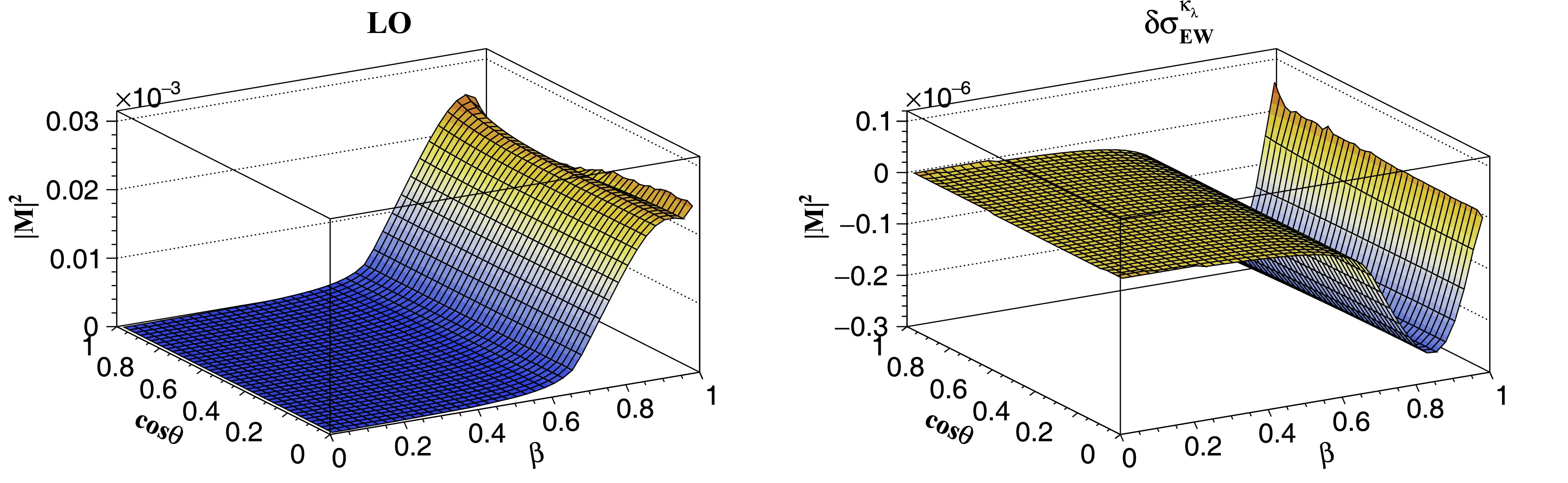
Figure 2. (color online) LO squared amplitudes (left) and
$ \lambda $ dependent EW corrections (right).The LO cross section of the VBF channel also exhibits a quadratic dependence on the trilinear Higgs coupling. The higher power dependence can be obtained by calculating the one-loop diagrams with an additional Higgs propagator. The calculation procedure is standard except for the renormalization, as explained above. We implemented the analytical results using the proVBFHH program [41, 68]. We employed the QCDLoop package [69] to evaluate the scalar one-loop integrals.
-
In our numerical calculations, we set
$ v=(\sqrt{2}\,G_F)^{-1/2} $ with the Fermi constant$ G_F=1.16637\times 10^{-5}\,\rm GeV^{-2} $ , the Higgs boson mass$ m_H=125 $ GeV, and the top quark mass$ m_t=173 $ GeV. For the VBF channel, we set the EW gauge boson masses as$ M_W=80.379 $ GeV and$M_Z= 91.1876$ GeV. We used the$\rm PDF4LHC15\_ {\rm{nlo\_100\_pdfas}}$ PDF set [70] and the associating strong coupling$ \alpha_s $ . The default renormalization scale in$ \alpha_s $ and factorization scale in the PDF were chosen to be$ \mu_{R, F}=m_{HH}/2 $ in the ggF channel and$ \mu_{R, F}=\sqrt{-q_i^2} $ in the VBF channel, with$ m_{HH} $ being the Higgs pair invariant mass and$ q_i $ being the transferred momenta from quark lines.The EW corrections that contain higher power dependence on the Higgs self-coupling are given by
$ \begin{aligned}[b] \delta\sigma^{\kappa_{\lambda}}_{{\rm{ggF,EW}}} =\;& (0.075\kappa_{\lambda_{{\rm{3H}}}}^4-0.158\kappa_{\lambda_{{\rm{3H}}}}^3-0.006\kappa_{\lambda_{{\rm{3H}}}}^2\kappa_{\lambda_{{\rm{4H}}}}\\ &-0.058\kappa_{\lambda_{{\rm{3H}}}}^2 +0.070\kappa_{\lambda_{{\rm{3H}}}}\kappa_{\lambda_{{\rm{4H}}}} -0.149\kappa_{\lambda_{{\rm{4H}}}})\; \; {{\rm{fb}}} \end{aligned} $

(12) for the ggF channel and
$ \begin{aligned}[b] \delta\sigma_{{\rm{VBF,EW}}}^{\kappa_\lambda}=\;&(0.0215\kappa_{\lambda_{{\rm{3H}}}}^4-0.0324\kappa_{\lambda_{{\rm{3H}}}}^3-0.0019\kappa_{\lambda_{{\rm{3H}}}}^2\kappa_{\lambda_{{\rm{4H}}}}\\ &-0.0043\kappa_{\lambda_{{\rm{3H}}}}^2 +0.0151\kappa_{\lambda_{{\rm{3H}}}}\kappa_{\lambda_{{\rm{4H}}}}-0.0211\kappa_{\lambda_{{\rm{4H}}}})\; \; {{\rm{fb}}} \end{aligned} $

(13) for the VBF channel. We computed all the
$\mathcal{O}(\lambda_{{\rm{3H}}}^i),\; i\ge 2$ contributions in the amplitude. The above$ \kappa_{\lambda_{{\rm{3H}}}}^2 $ terms arise because we aimed to keep the cancellation relation between the$ \mathcal{O}(\lambda_{{\rm{3H}}}) $ and$ \mathcal{O}(1) $ amplitudes at LO. The cubic$ \kappa_{\lambda_{{\rm{3H}}}}^3 $ and quartic$ \kappa_{\lambda_{{\rm{3H}}}}^4 $ terms appear for the first time up to this perturbative order. Although their coefficients are small, they provide notable corrections to the cross section if$ \kappa_{\lambda_{{\rm{3H}}}} $ is chosen to be much larger than 1. As shown in Table 1, the$ \lambda $ dependent corrections in the ggF (VBF) channel reach 91% (82%) of the LO cross section for$ \kappa_{\lambda_{{\rm{3H}}}}=6 $ .$ \kappa_{\lambda_{{\rm{3H}}}} $ 

$ \kappa_{\lambda_{{\rm{4H}}}} $ 

ggF VBF $ \sigma_{{\rm{LO}}}^{\kappa_{\lambda}} $ 

$ \sigma_{{\rm{NNLO-FT}}}^{\kappa_{\lambda}} $ 

$ \delta\sigma^{\kappa_\lambda}_{{\rm{EW}}} $ 

$ \sigma_{{\rm{LO}}}^{\kappa_{\lambda}} $ 

$ \sigma_{{\rm{NNNLO}}}^{\kappa_\lambda} $ 

$ \delta\sigma^{\kappa_\lambda}_{{\rm{EW}}} $ 

1 1 16.7 31.2 −0.225 1.71 1.69 $ -2.30 \times 10^{-2} $ 

3 1 8.59 18.4 1.28 3.59 3.53 $ 8.35\times 10^{-1} $ 

6 1 67.3 161 60.6 25.1 24.6 20.7 1 3 16.7 31.2 −0.393 1.71 1.69 $ -3.89 \times 10^{-2} $ 

1 6 16.7 31.2 −0.646 1.71 1.69 $ -6.27 \times 10^{-2} $ 

3 3 8.59 18.4 1.30 3.59 3.53 $ 8.50\times 10^{-1} $ 

6 6 67.3 161 61.0 25.1 24.6 20.7 Table 1. Cross sections (in fb) of ggF and VBF Higgs boson pair production for different values of
$ \kappa_{\lambda_{{\rm{3H}}}} $ and$ \kappa_{\lambda_{{\rm{4H}}}} $ at the 13 TeV LHC.In addition, there is a new dependence on the quartic Higgs self-coupling
$ \lambda_{{\rm{4H}}} $ . Because this dependence is only linear and the corresponding coefficients are small, their contributions are negligible. According to Table 1, the cross section varies by 0.6% when$ \kappa_{\lambda_{{\rm{4H}}}} $ changes from 1 to 6 while keeping$ \kappa_{\lambda_{{\rm{3H}}}}=6 $ . As a consequence, we do not expect that a meaningful constraint on the quartic Higgs self-coupling can be extracted from Higgs boson pair production at the LHC.Next, we compare our results with those reported in Refs. [31, 71]. The authors of these papers obtained similar expressions for the cross sections in the ggF channel. However, they assumed that the triple and quartic Higgs self-couplings are modified by one dimension-six and one dimension-eight operators
2 . They performed calculations, especially renormalization, in terms of the coefficients of higher-dimensional operators and then transformed the results onto the basis of$ \kappa_{\lambda_{{\rm{3H}}}} $ and$ \kappa_{\lambda_{{\rm{4H}}}} $ . These results cannot be directly compared with the experimental analysis in the$ \kappa $ framework.Fig. 3 shows different perturbative predictions for the cross sections of both ggF and VBF Higgs boson pair productions at the 13 TeV LHC as a function of
$ \kappa_{\lambda_{{\rm{3H}}}}=\kappa_{\lambda_{{\rm{4H}}}}=\kappa_{\lambda} $ . It is evident that higher-order perturbative corrections dramatically change the functional form. The current experimental upper limit set by the ATLAS (CMS) collaboration on$ \kappa_{\lambda} $ is$ 6.6 $ (6.49) based on the theoretical predictions at QCD NNLO in the ggF channel and NNNLO in the VBF channel; see Table 1. Taking$ \delta\sigma^{\kappa_\lambda}_{{\rm{EW}}} $ corrections into account and assuming that the QCD and EW corrections are factorizable, the upper limit is narrowed down to 5.4 (5.37). These limits are almost the same when keeping$ \kappa_{\lambda_{{\rm{4H}}}}=1 $ . If the scale uncertainties are considered [74], the upper limit would span in the range$(6.5,~6.8)$ for the ATLAS results, which would decrease to$(5.4,~5.6)$ after including higher power dependence. Concerning the CMS results, the upper limit changes from (6.40, 6.67) to (5.31, 5.48). The lower limits are only slightly modified.
Figure 3. (color online) Cross sections of Higgs boson pair production at the 13 TeV LHC including both ggF and VBF processes as a function of
$ \kappa_{\lambda_{{\rm{3H}}}}=\kappa_{\lambda_{{\rm{4H}}}}=\kappa_{\lambda} $ . The black line represents the LO results, whereas the green line denotes the results with (N)NNLO QCD corrections in the ggF (VBF) channel. The red line indicates the results including higher power dependence on the Higgs boson self-coupling. The current and improved upper limits are labeled by points A and B, respectively.Lastly, the Higgs boson pair invariant mass
$ m_{HH} $ distributions are shown in Fig. 4. The peak position moves from 400 GeV to 260 GeV when$ \kappa_{\lambda} $ varies from 1 to 6, which indicates that the Higgs bosons tend to be produced with very low velocity in the case of large$ \kappa_{\lambda} $ values. This feature could help set optimal cuts in the experimental analysis to enhance sensitivity. From this figure, we also observe that the$ \lambda $ dependent corrections have a great impact on the distributions, especially in the small$ m_{HH} $ region. Therefore, they should be included in future studies.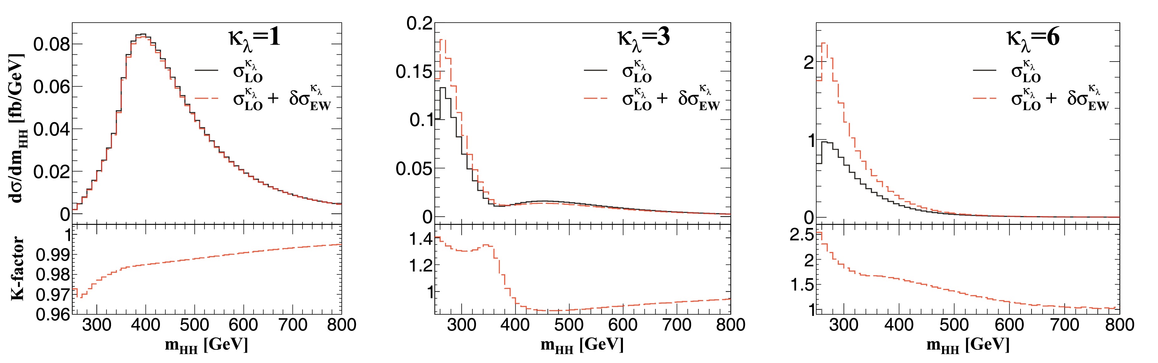
Figure 4. (color online) Higgs boson pair invariant mass distributions at LO and with
$ \delta\sigma_{{\rm{EW}}}^{\kappa_\lambda} $ corrections at the 13 TeV LHC. We set$ \kappa_{\lambda_{{\rm{3H}}}}=\kappa_{\lambda_{{\rm{4H}}}}=\kappa_{\lambda} $ . -
The precise shape of the Higgs potential constitutes a fundamental enigma in particle physics. The current limits on the Higgs self-coupling are predominantly derived under the assumption that the cross section of the Higgs boson pair production is a quadratic function of the self-coupling. We found that the functional form should be generalized to include quartic and cubic power dependencies on the Higgs self-coupling that arise from higher-order quantum corrections induced by virtual Higgs bosons.
We propose a proper renormalization procedure to explicitly retain the Higgs self-couplings at each calculation step and introduce renormalization of the coupling modifiers to ensure the cancellation of all ultraviolet divergences. We present numerical results of the cross sections of both the ggF and VBF channels at the LHC including higher power dependencies on the Higgs self-coupling. With these improved functional forms, we demonstrate that the upper limit set by the ATLAS (CMS) collaboration on the trilinear Higgs self-coupling normalized to its SM value can be reduced from 6.6 (6.49) to 5.4 (5.37). This more precise constraint is achieved without analyzing additional data, underscoring the critical importance of incorporating higher power dependencies on the Higgs self-coupling in the cross section.
Furthermore, we found it difficult to derive any useful constraint on the quartic Higgs self-coupling solely from Higgs boson pair production. To probe the quartic self-coupling, alternative channels such as triple Higgs boson production may be explored, necessitating collider facilities with energies higher than those of the LHC to provide insights into this aspect of the Higgs potential.
-
We express our gratitude to Huan-Yu Bi, Yan-Qing Ma, and Huai-Min Yu for comparing the numerical results of the two-loop amplitudes. We also thank Shan Jin, Yefan Wang, and Lei Zhang for helpful discussions.
Improved constraints on Higgs boson self-couplings with quartic and cubic power dependencies of the cross section
- Received Date: 2024-11-12
- Available Online: 2025-02-15
Abstract: Precise determination of the Higgs boson self-couplings is essential for understanding the mechanism underlying electroweak symmetry breaking. However, owing to the limited number of Higgs boson pair events at the LHC, only loose constraints have been established to date. Current constraints are based on the assumption that the cross section is a quadratic function of the trilinear Higgs self-coupling within the


 DownLoad: