QED effects on Kerr-Newman black hole shadows

Since the groundbreaking achievement of capturing the first two images of supermassive black holes (M87* and Sgr A*, respectively) by the Event Horizon Telescope (EHT) [1–6], the field of black hole physics has entered a new era. This achievement not only provided direct confirmation of the existence of black holes but also unveiled a wealth of information about these enigmatic cosmic entities and their surrounding environments. A central focus of research has been the black hole shadow [1, 7], a prominent feature of black hole images. The precise shape of this shadow has been shown to encode critical physical parameters, such as the mass and spin of the black hole [2, 8–15]. Furthermore, the study of black hole shadows has proven instrumental in addressing fundamental questions spanning a broad spectrum of topics, such as the behavior of accretion disks [16–20], the nature of dark matter [21–25], the dynamics of an accelerating universe [26, 27], modified gravity theories [28–34], and the existence of extra dimensions [35, 36]. These intriguing questions have ignited a surge of theoretical and experimental research into black hole shadows.

Theoretical investigations on black hole shadows primarily rely on our understanding of photon trajectories in the spacetime surrounding black holes. In a vacuum, photons travel along geodesics under the approximation of geometric optics. Thus, the equations of motion of photons are completely governed by the spacetime background. However, there will inevitably be other fields besides the gravitational field in real spacetime. Therefore, a realistic possible scenario is that photons interact with other fields as they travel outside the black hole. Magnetic fields are of particular significance, playing a crucial role in the physics of black holes [37–42]. Observations have indicated the presence of strong magnetic fields around supermassive black holes, which may result in the breakdown of the superposition principle. The electromagnetic field exhibits self-interaction; in other words, photon-photon interactions become significant. This leads to nonlinear QED corrections to electrodynamics, making the electromagnetic field behave as if it were some kind of electromagnetic medium—a phenomenon known as vacuum polarization. Rays of light traveling within the electromagnetic field deviate from null geodesic paths and follow different timelike trajectories depending on their polarization direction, resulting in what is known as birefringence phenomenon [43, 44].

Nonlinear electrodynamics effects emerge in different models, with the Euler-Heisenberg model [45–47] and the Born-Infeld-like models [47–53] being the most renowned among them. The former one is a result of one-loop quantum corrections [54], while the latter was proposed as a solution of the divergence of the self-energy of a point charge [55]. The additional nonlinear terms in electrodynamics introduce extra terms in the energy-momentum tensor, thereby indirectly affecting the trajectory of light by modifying the spacetime geometry [56]. It is challenging to construct a fully backreacted black hole solution and study novel features in its image.

In this study, we aimed to explore the influence of QED effects by examining a simplified scenario involving a rotating charged black hole. Specifically, we considered a Kerr-Newman-like black hole with a magnetic charge, taking into account the linear effect of QED on the spacetime geometry. After analyzing both the direct impact of the electromagnetic field on light trajectories and the distortion of the background spacetime metric caused by QED corrections, we obtained the shadow of the black hole.

Remarkably, we found that the area of the black hole shadow increases with the QED corrections, which is in conflict with results previously reported [52, 57, 58]. The discrepancy originates from a sign difference in the photon Hamiltonian. In simple terms, the resulting photon trajectories should be timelike. However, because of the wrong sign, they have been reported to be spacelike in the literature. Thus, one of the motivations of the present study was to correct the errors in [57, 58] reported by two of the authors (Z.Z. Hu and B. Chen) with others.

This manuscript is structured as follows. In Sec. II, we provide a concise overview of the Euler-Heisenberg Lagrangian along with its resulting dispersion relations. We correct an essential sign error made in previous studies [52, 57, 58]. In Sec. III, we consider the modifications to spacetime geometry due to the additional energy-momentum tensor of the electromagnetic field. In Sec. IV, we examine the QED influence on the shape of the shadow and discuss the contributions of different mechanisms of QED effects. In Sec. V, we summarize our findings. Additionally, some detailed formulas and derivations are presented in Appendices A, B, and C.

As shown in [53], by considering one-loop vacuum polarization, the Euler-Heisenberg effective Lagrangian for the electromagnetic field (in Gaussian units) can be expressed as

where the variables $ \mathcal{F} $ and $ \mathcal{G} $ are the only two independent relativistic invariant and pseudo-invariant constructed from the Maxwell field in four dimensions,

The coefficient $ \mu $ reads

with $ \hslash $, $ \alpha $, and $ m_e $ being the Planck constant, fine-structure constant, and electron mass, respectively. We assume geometric units in this paper, setting $ c=G=1 $. We also set $ M=1 $ for simplicity. In this case, $ \mu $ is not a constant anymore because the physical constants there have dimensions, e.g., $ \hslash $ is proportional to $ m_{p}^{2} $. The numerical value of $ \mu $ in geometric units can be calculated from

where $ M_\odot $ represents the mass of the sun. Therefore, in the rest of the paper, when we change the value of $ \mu $, we will be really varying the mass of the black hole $ M $ in our geometric units.

According to previous studies, we can derive the modified equations of motion from the effective Lagrangian using the effective metric. The derivation of an accurate expression for the effective metric is complicated; it is provided in Appendix A. At the first order of approximation in $ \mu $, the invariant effective metric tensor with upper index is

with

The choice of $ \lambda $ is determined by the polarization of the photon because the one-loop vacuum polarization makes the electromagnetic field an anisotropic dielectric. Then, the effective metric tensor with lower indices is defined to be the inverse of $ \tilde{G}^{\alpha\beta} $,

To the leading order of $ \mu $, we have

With the dual vector $ q_\mu $ being defined as $ \tilde{G}_{\mu\nu} p^\nu $, the Hamiltonian and Hamiltonian equations read

Note trom the above equations that the photon effectively becomes a timelike particle in the original spacetime,

Intuitively, this is reasonable: the trajectories of photons can no longer remain lightlike given that they are no longer free massless photons. Instead, they become timelike under the constraint of causality. Accordingly, such interactions slow the photons down and make it easier for them to be trapped by the black hole. In other words, the gravitational traps of the photons enhance.

Even without gravity, QED birefringence alone can trap photons, as shown in [44], where this effect was referred to as "electromagnetic traps". Intuitively, the stronger the electromagnetic field is, the larger the refractive index of the effective medium is, and the slower the photons are. As long as this strong electromagnetic field is local, i.e., the electromagnetic field attenuates to zero at infinity, the effective medium functions as a convex lens, converging the light rays, even trapping them, such that the black hole shadow may enlarge.

The deformation of the black hole shadows due to the QED effect was discussed in previous studies [57, 58]. However, there is a minus sign omitted in such studies, e.g., in Eq. (2.10) of [57], in comparison with Eq. (8), which would effectively appear as the opposite value of$ \lambda $ in the image of the result. All the related theoretical results must be corrected by substituting $ \lambda $ for $ -\lambda $. Consequently, the major features of the images are also opposite.

Corrected calculations from [57] are briefly explained next. As in Sec. IV of [57], we consider a Schwarzschild black hole immersed in a uniform magnetic field,

The corrected effective metric is given by

where $ f\left(r\right)\equiv1-2/r $ is the redshift factor of an ordinary Schwarzschild black hole, and the positive dimensionless quantity $ \Lambda $ is defined as

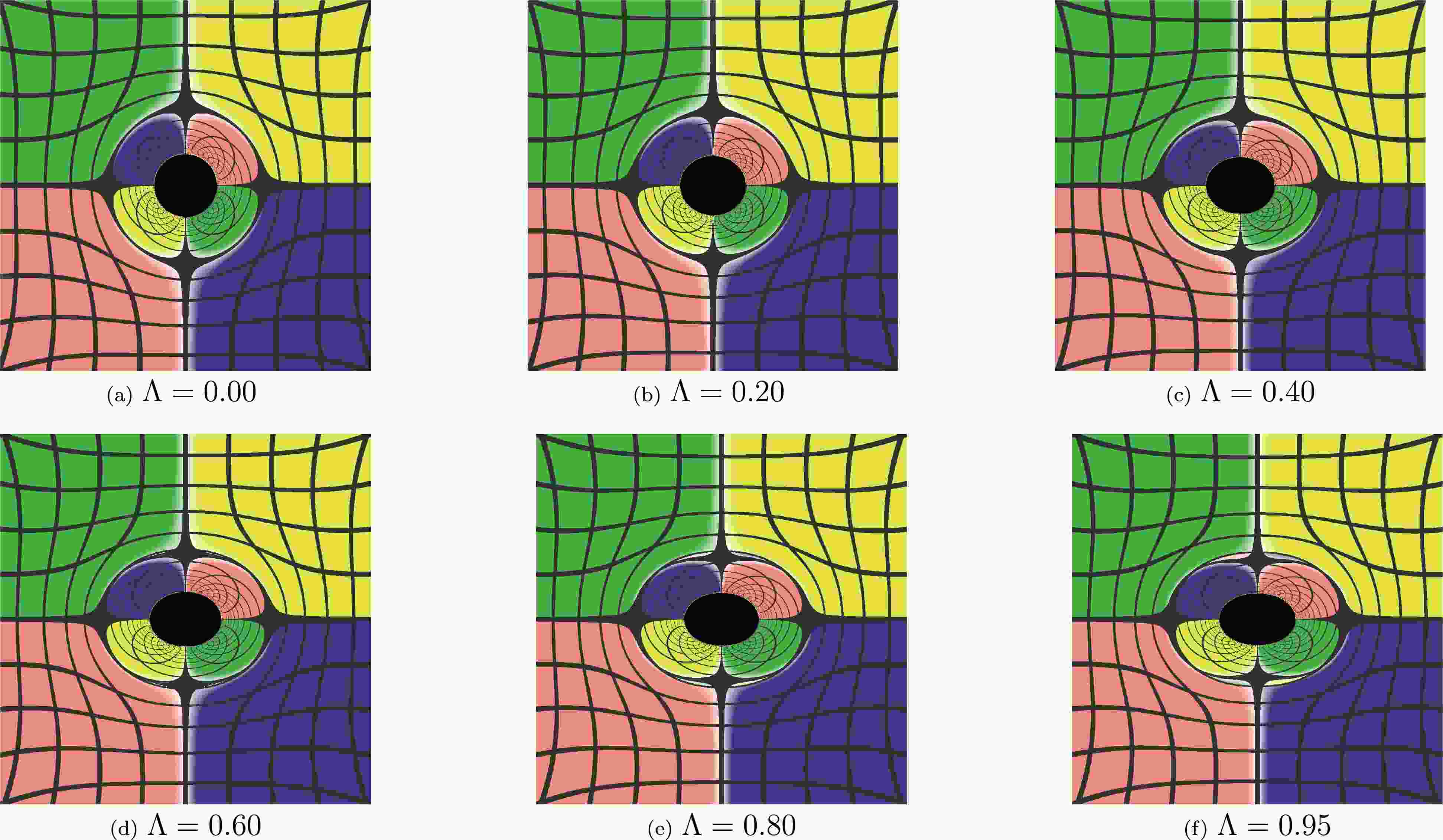
The dimensionlessness of $ \Lambda $implies the invariance of its expression under unit change; in other words, its expression in SI units remains unchanged. Consequently, the absolute strength of the magnetic field$ B $ turns out to be the only quantity that affects the shape of black hole shadows in this static model, while the black hole mass $ M $ has no effect on it. The corrected images of the static black hole in uniform magnetic fields are shown in Figs. 1 and 2, which should be compared with Figs. 3 and 4 (i.e., Figs. 3 and 7 in [57]), respectively. Notably, the magnetic field is horizontally set in the images. The comparison shows that the shadows are stretched in the direction of the magnetic field and squeezed in the perpendicular direction rather than the other way around. Similar recalculations and discussions about results reported in [58] can be carried out as well, focusing on rotating black holes in magnetic fields.

Figure 1.  (color online) Images of the static black hole in uniform magnetic fields. The inclination angle of the observer is fixed at $ \theta_o=\pi/2 $.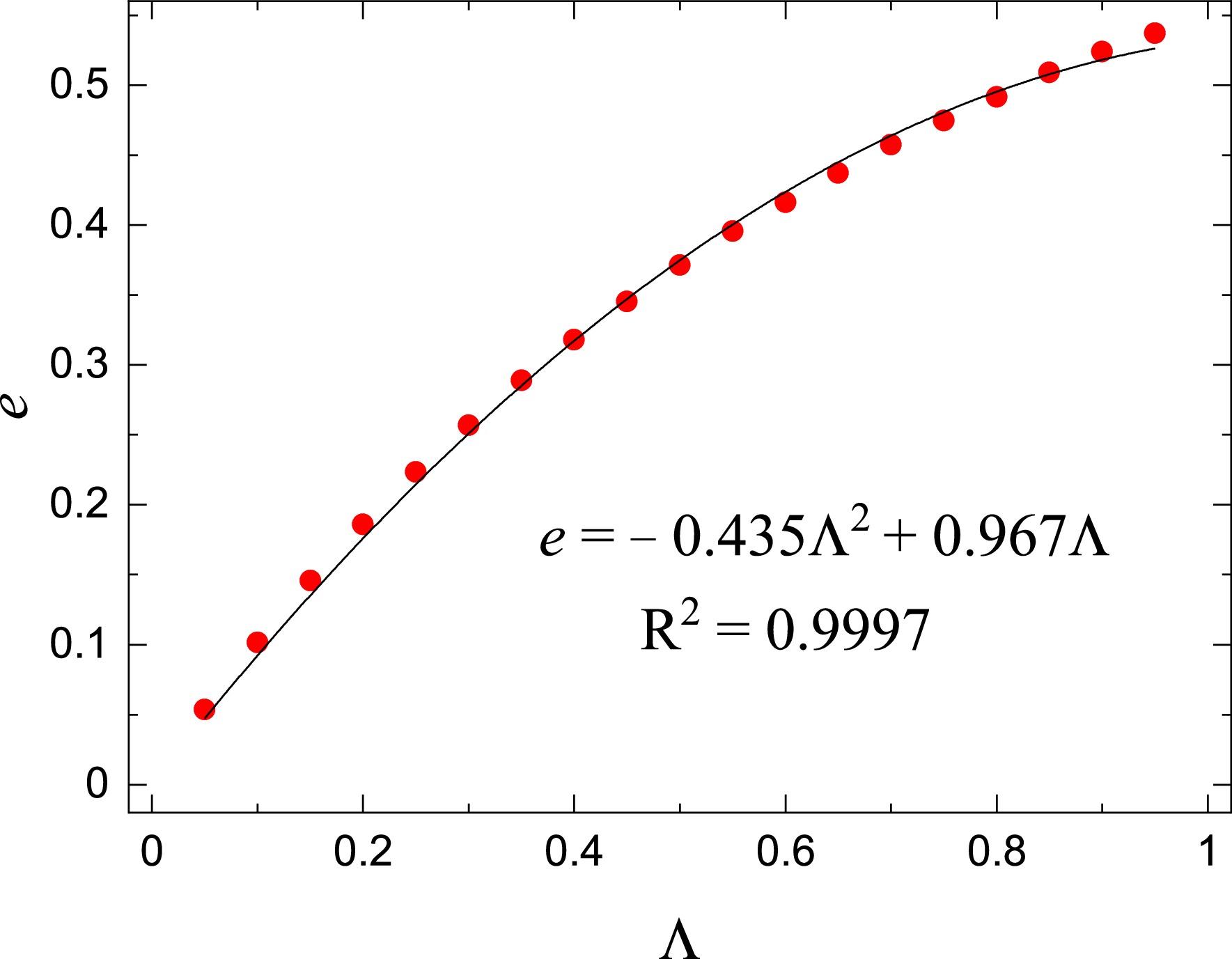

Figure 2.  (color online) Variation of the eccentricity of the image concerning $ \Lambda $. A quadratic function was employed to fit the data.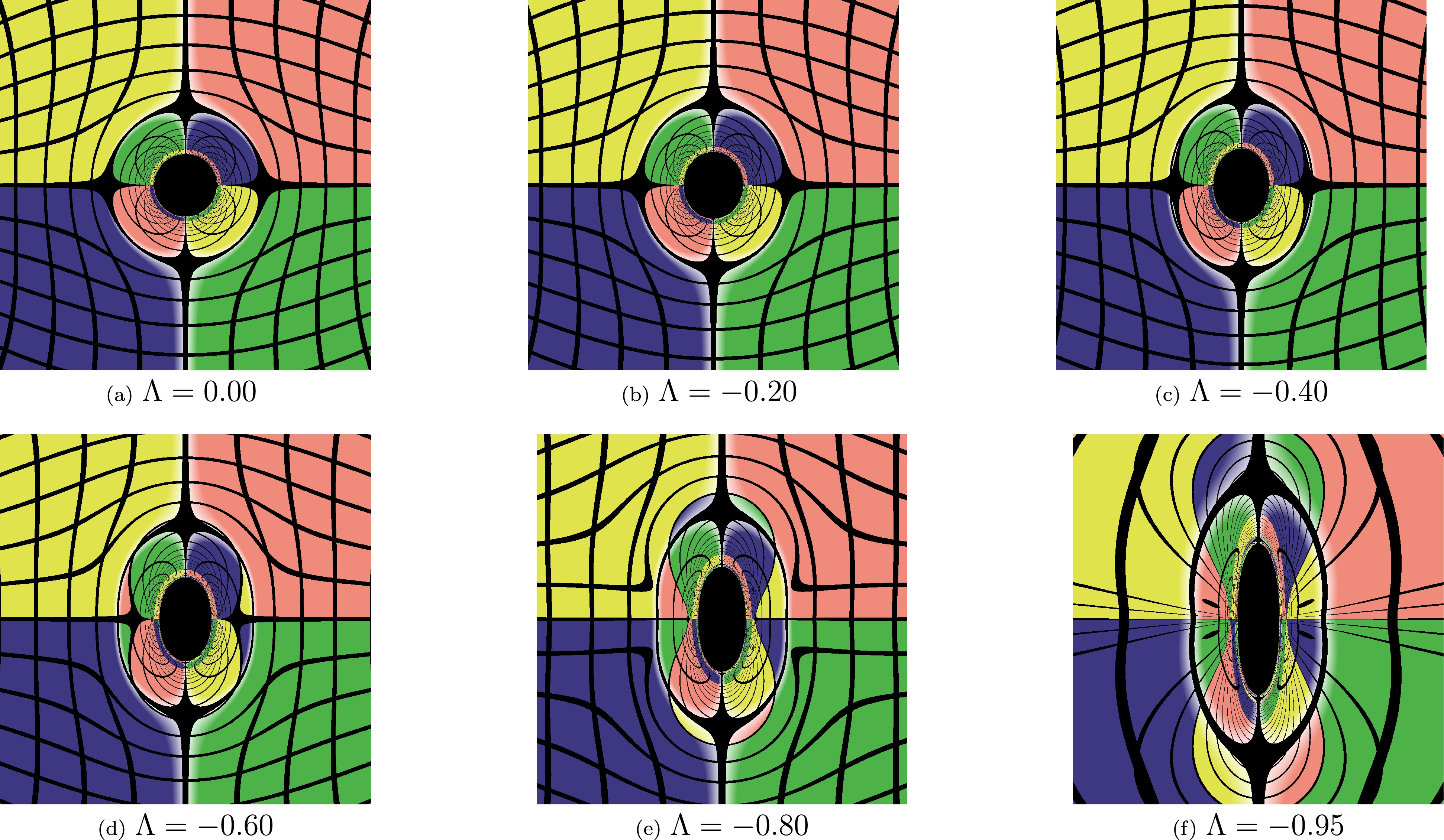

Figure 3.  (color online) Figure 5 in Ref. [57].

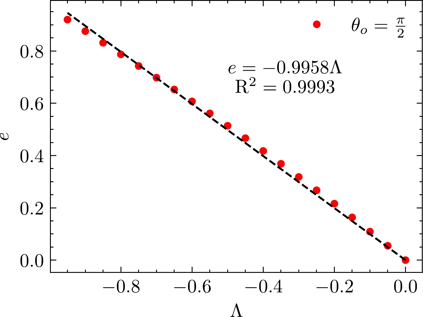
Figure 4.  (color online) Figure 7 in Ref. [57].

Another group conducted research under similar settings [52] and obtained the opposite conclusion on the black hole shadow. Similar to [57, 58], the authors in [52] made the same mistake on the sign of $ \lambda $. Similar to any normal GR physicists, they used the "East Coast" metric, i.e., $ \eta=\mathrm{diag}(-,+,+,+) $. However, they employed the same expression for the effective metric, $\tilde{G}^{\mu\nu}= g^{\mu\nu}+\dfrac{16\alpha^2\hslash^3}{45m_e^4}T^{\mu\nu}$, from [59], which is written in the "West Coast" metric, i.e., $ \eta=\mathrm{diag}(+,-,-,-) $. Under this notation shift, the spacetime metric $ g^{\mu\nu} $ shows a sign flip, while the energy-momentum tensor $ T^{\mu\nu} $ does not. Therefore, the right expression in line with the "East Coast" metric should be $ \tilde{G}^{\mu\nu}=g^{\mu\nu}-\dfrac{16\alpha^2\hslash^3}{45m_e^4}T^{\mu\nu} $, which agrees with Eq. (5) for $ \lambda=-8\mu $ up to a conformal factor (see Appendix A). Unfortunately, the authors did not introduce the corresponding changes in [52] and used the wrong sign of $ \lambda $, which led to an opposite conclusion: black hole shadows shrink under QED effects.

To consider the backreaction of the QED effect, we need to study the Einstein equation,

where

For a static and spherically symmetric black hole with electric charge or magnetic charge only, its metric can be solved analytically [56, 60],

where

and $ Q $ is either the electric or magnetic charge. This black hole is referred to as the QED-RN black hole in this paper. Notice that

The fact that ${\mathop\lim\limits}_{r\to\infty}m(r)=1=M$ indicates that $ M $ represents the full mass in space, including the energy of the electromagnetic field. Accordingly, with $ M $ fixed, a larger value of $ Q $ means stronger electromagnetic fields. As the effective mass decreases with increasing $ Q $, the shadows of classical RN and QED-RN black holes become smaller with increasing $ Q $. However, it is remarkablethat the shadow of QED-RN black holes is larger than that of RN black holes with the same charge $ Q $. This is owing to the fact that the QED effect screens the charge $ Q^2 \to Q^2 -\mu Q^4/(10\pi r^4) $ such that the "gravitational mass" of electromagnetic fields is reduced and the remaining gravitational mass becomes larger. In other words, the QED backreaction correction tends to enlarge the shadow.

Unfortunately, when it comes to rotating cases, an exact solution has not been found yet. Nevertheless, we proceed with the solution found in [56], which is generated from the static one by using the Newman-Janis algorithm. The solution can be expressed in terms of the Gürses-Gürsey metric [61],

where

The parameter $ Q $ can be either electric charge $ Q_e $ or magnetic charge $ Q_m $. The outer horizon is still the largest root of $ \Delta=0 $, i.e.,

which is determined by $ a $, $ Q $, and $ \mu $together. Remarkably, the Newman-Janis algorithm is accurate only with linear sources. Because of the nonlinearity caused by QED effects, the above solution is only an approximation. Further discussion can be found in Appendix B.

The fact that the Gürses-Gürsey metric can simply be obtained from the classical Kerr-Newman metric by using the substitute $ Q^2 \to Q^2-\mu Q^4/(10\pi r^4) $ was interpreted as a screening effect in [62], as in the spherical case. Similar arguments were employed in [52], although with a different algebraic expression describing this effective screening. However, this variation does not qualitatively affect the conclusions.

As in the spherical case, the term "effective screening" really means that the QED effect reduces the "gravitational mass" of electromagnetic fields. According to Eq. (15), the QED correction term in the energy-momentum tensor of electromagnetic fields reads

which violates the strong energy condition (SEC) as well as the null energy condition (NEC), as shown in Appendix C. More explicitly, the energy density of the QED correction term tends to be negative and reduces the gravitational energy of the electromagnetic fields. In this sense, we would expect the backreaction effect to enlarge the shadow, even at the nonlinear level.

It was demonstrated in [56] that, in the framework of nonlinear electrodynamics, the natural variables are the dual Plebański variables ($ P_{\mu\nu} $) when considering electrically charged black holes, and the standard Maxwell variables ($ F_{\mu\nu} $) when considering magnetically charged black holes. We have not found a good method to analyze the case with both charges yet. Given that these two cases are similar, we mainly focused on the magnetically charged case in this study, leaving the electrically charged case for future study. Regarding the magnetic case, we can directly obtain the solution of Maxwell variables [56] as follows:

Generally speaking, the geodesic equation in spacetime generated from a static spherically symmetric metric through the Newman-Janis algorithm can be separated completely [63]. However, we are considering the effective metric in Eq. (8), which destroys the separability of the corresponding Hamilton-Jacobi equation. Therefore, we applied the numerical backward ray-tracing method proposed in [57] in this study. The requisite setup includes background space-time [Eqs. (19) and (20)], the electromagnetic field [Eq. (24)], and the photon's equation of motion [Eqs. (8) and (9)]. We also employed the stereographic projection, which is often called the fisheye camera model. The details can be found in the Appendix of [57]. Using these methods, we simulated the image of the black hole with a shadow in the middle.

In our geometric units, the mass $ M $ is set to 1, and alternatively the coefficient $ \mu $ is variable, as explained in Sec. II. Moreover, $ Q_{e} $ is set to zero for simplicity. To establish a more significant difference between the shadows with and without QED effects, we determine the polarization of photons by setting $ \lambda=-14\mu $, i.e., $ \Omega=\Omega_- $. Therefore, our three independent parameters are $ a $, $ Q_m $ and $ \mu $. When we set $ \mu=0 $, we move back to the classical Kerr-Newman case.

For a backreacted KN black hole, the larger $ \mu $ is, the smaller the mass is, the stronger the QED effects are, and the larger the shadows are. In Fig. 5, we compare the images of the black hole for two different values of $ \mu $; the QED effect in expanding the shadow of a black hole is evident. Similarly, increasing $ Q_m $ leads to stronger electromagnetic fields and hence stronger QED effects and larger expansion in shadows. In contrast, the effects of altering $ a $ are comparatively small in a large parameter space range, as will be shown in Subsec. IV.A.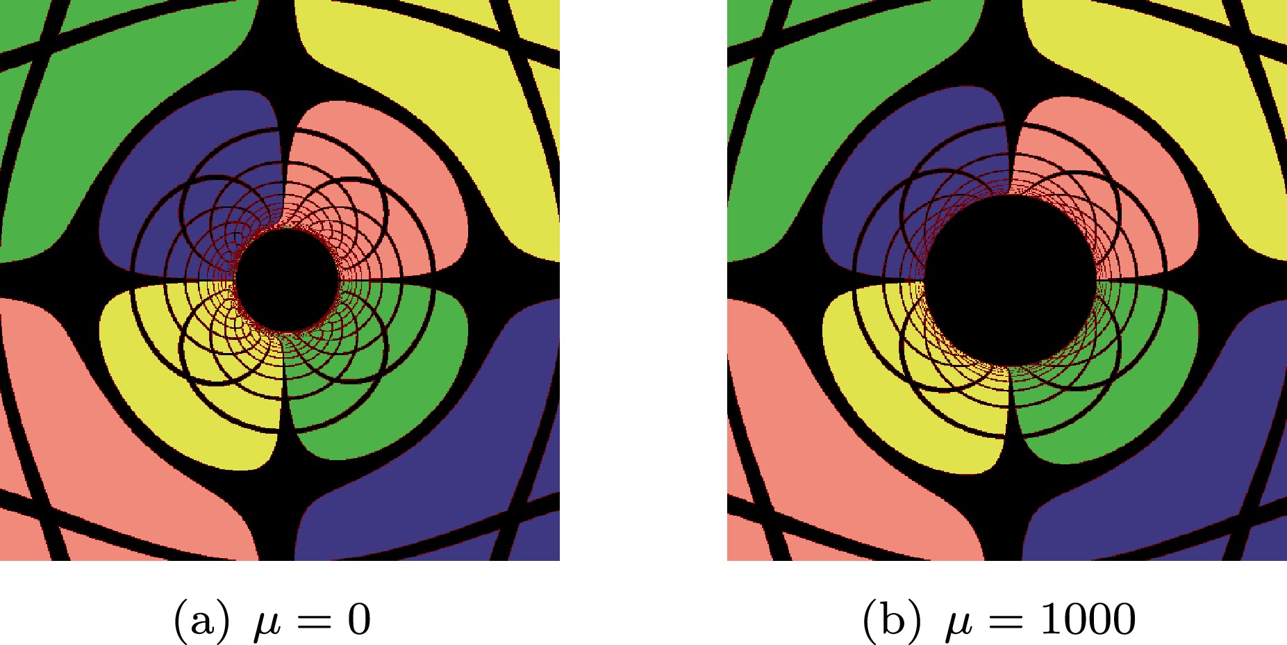

Figure 5.  (color online) Images of the charged spinning black hole with different QED coupling strength. The inclination angle of the observer is fixed at $ \theta_o=\pi/2 $, the magnetic charge is $ Q_m=0.6 $, and the spin is $ a=0.3 $.

Roughly speaking, larger $ \mu $ means stronger QED coupling, larger $ Q_m $ leads to sa tronger electromagnetic field, and hence larger $ \mu $ and large $ Q_m $ jointly give rise to larger QED effects. To investigate their impact on the shadows quantitatively, we can introduce a few geometry parameters suggested in [19, 30, 58] as follows. The center of the shadow is defined to be

The polar coordinates ($ \tilde{r} $,$ \alpha $) can be defined with respect to the center of the shadow as

Then, the area of the shadow can be calculated from

which can be normalized by the shadow area of the corresponding KN black hole ($ \mu=0 $) as

The ratio $ S/S_0 $ indicates the expansion of shadows induced by QED corrections. Additionally, the QED-induced deviation from the corresponding KN black hole ($ \mu=0 $) is characterized by

With the parameters defined above, we can discuss the strength of QED effects and its dependence on $ \mu $, $ Q_m $, and $ a $ quantitatively. In Fig. 6, we show how the expansion $ S/S_0 $ and deviation $ \sigma_K $ vary with respect to different values of $ \mu $, $ Q_m $, and $ a $. In this study, we varied only one parameter and kept the other two parameters fixed. We found that the expansion effects of QED corrections take place through decelerating growth with increasing $ \mu $ and approximately linear growth with increasing $ Q_m $, respectively. (Notice that we use a logarithmic coordinate for $ \mu $ because of its wide range of variation.) In contrast, the QED expansion effects remain basically invariant with increasing $ a $, though a slight enhancement is still observable. Moreover, we found another relation with very high precision, $ S/S_0\approx\left(\sigma_K+1\right)^2 $, which reflects the fact that the black hole shadow is approximately a circle, even for relatively large values of $ a $.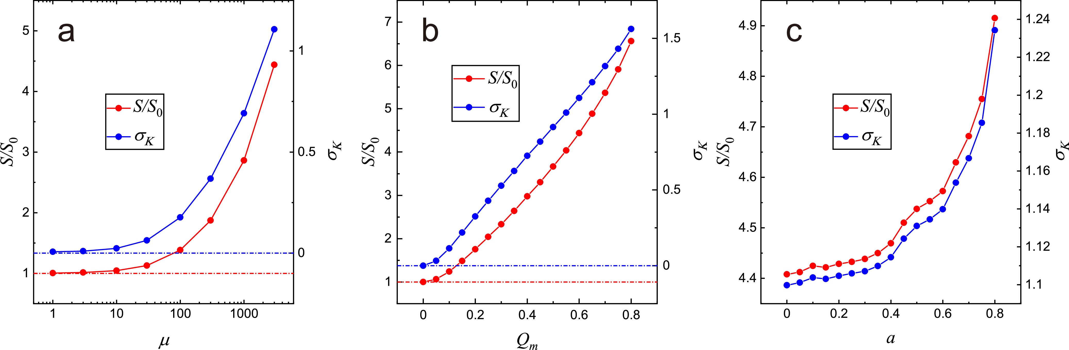

Figure 6.  (color online) Variation of geometry parameters for different values of $ \mu $, $ Q_m $, and $ a $. $ S $ refers to the area with given $ \mu $, and $ S_0 $ refers to that with $ \mu=0 $;$ \sigma_K $ refers to the "normalized" deviation between given $ \mu $ and $ \mu=0 $. (a) $ S/S_0-\mu $ and $ \sigma_K-\mu $ with $ a=0.3 $ and $ Q_m=0.6 $. (b) $ S/S_0-Q_m $ and $ \sigma_K-Q_m $ with $ a=0.3 $ and $ \mu=3000 $. (c) $ S/S_0-a $ and $ \sigma_K-a $ with $ Q_m=0.6 $ and $ \mu=3000 $.

In this and the next subsection, we will distinguish two different effects of 1-loop QED correction to the black hole shadow. The first one is the backreaction effect to the spacetime geometry; the other is the QED birefringence effect, leading to QED enhanced gravitational traps as well as electromagnetic traps [44], as explained in Sec. II.

Let us first investigate the contribution of the backreaction effects. We simply have to compare the black hole shadows with and without the backreaction. Similar to Subsec. IV.A, we define the geometrical parameters as

and

where $ \tilde{r}^*\left(\alpha\right) $ refers to the shadow curve without considering the backreaction. The numerical results are shown in Fig. 7. These results show that the backreaction enlarges the shadow, which agrees with our discussion in Sec. III. However, the backreaction effect is extremely small and can be neglected, as argued in [52].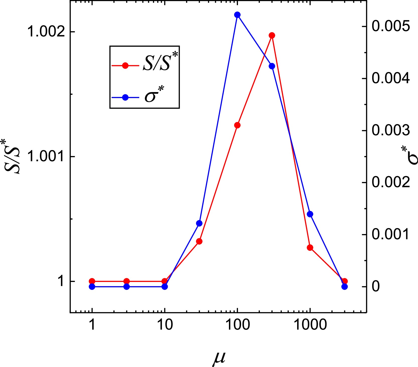

Figure 7.  (color online) Demonstration of the contrast between the shadows with and without backreaction to the spacetime. We set $ a=0.3 $ and $ Q_m=0.6 $; $ S $ refers to the area of shadows of given $ \mu $ with backreaction to the background spacetime; $ S^* $ refers to that without backreaction; $ \sigma^* $ refers to the "normalized" deviation between the corresponding shadows.

Another interesting point is that the deviation between the shadows with and without background spacetime modification increases with $ \mu $ at small coupling and then decreases. Their growth at small coupling is intuitively expected. When QED effects, which enlarge the shadows, become sufficiently strong, photons traveling to infinity can no longer pass through small $ r $ regions. Note that the background spacetime modification, i.e., the screening term described in Sec. III, exhibits a quartic attenuation with respect to $ r $. Therefore, the modification becomes less important.

As explained in Sec. II, the QED birefringence effects make the trajectory of the photon timelike rather than null. Effectively, the photons travel in a medium with a refractive index larger than unity. If the electromagnetic field is local, the birefringence effects always enlarge the shadow, as shown in the case of a charged spinning black hole with QED corrections.

However, the situation becomes subtle if the electromagnetic field is uniformly distributed. In the case studied in [57], the black hole is immersed in a magneticfield extending uniformly to the infinity. As can be seen in Fig. 1, the shadow is stretched along the magnetic field while squeezed in the direction perpendicular to the magnetic field (note that the magnetic field is horizontal in Fig. 1). The areas of shadow for different values of $ \Lambda $ were computed; the results are plotted in Fig. 8. The area slightly decreases with increasing $ \Lambda $ at first but eventually grows rapidly for large values of $ \Lambda $.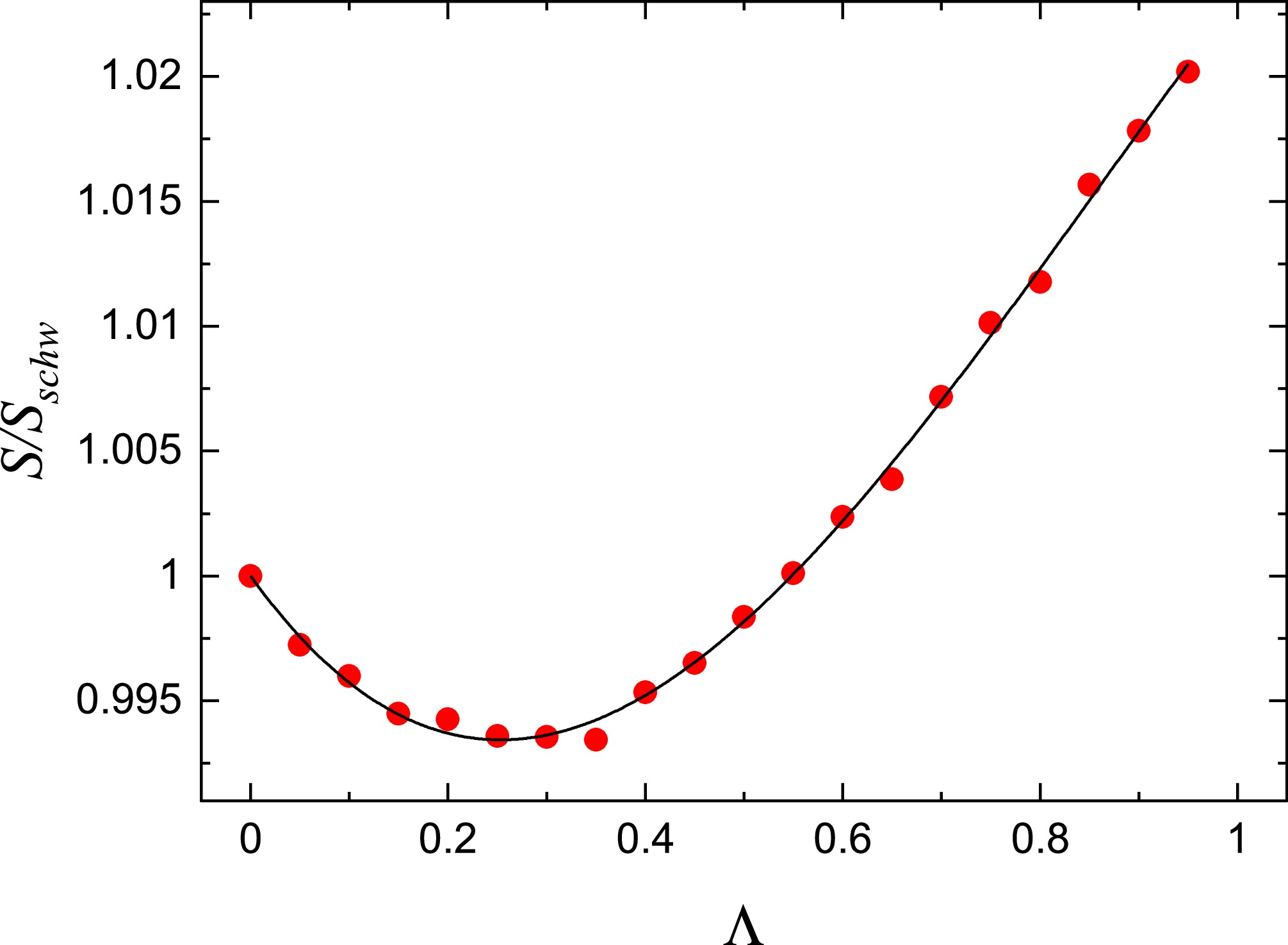

Figure 8.  (color online) Variation of the area of the shadow with respect to $ \Lambda $.

The perpendicular squeezing of the shadow as well as the initial decrease of the shadow area result from the presence of a uniform magnetic field. This can be understood more clearly in flat spacetime, in which case the effective refractive index does not decay to unity at infinity such that the light rays do not necessarily converge. It turns out that the uniform magnetic field tends to squeeze the shadow in a perpendicular direction. When $ \lambda $ is small, the squeezing may induce a decrease of the shadow area.

We conducted a study on the QED effects on the shadows of rotating black holes with magnetic charge. Two distinct QED effects were analyzed. One is the birefringence effect experienced by light rays in a strong electromagnetic field, whereas the other is the extra distortion of the background spacetime due to backreaction. We studied the impact of both effects on the black hole images and found that the QED effects tend to enlarge the shadows of black holes.

In practice, we implemented the ray-tracing algorithm to numerically simulate the shadow of black holes with different parameters. We defined two geometric parameters, namely the standard deviation of the area and radius, to characterize the expansion of black hole shadows quantitatively. The numerical results indicate that the QED-induced expansion of the shadows grows with the QED coupling $ \mu $ and magnetic charge $ Q_m $ while having relatively little dependence on spin $ a $.

We also analyzed the impact and contribution of different types of QED effects. We found that both the QED birefringence and backreaction effects tend to enlarge the shadow in our QED KN case. Moreover, our study demonstrates that the backreaction has an extremely small influence on the black hole images and could be neglected safely, supporting the rationality of previous studies [57, 58].

In [52], a similar topic was addressed. It was found that the shadows of black holes would shrink under QED effects, opposite to our conclusion. The discrepancy stems from the sign difference of $ \lambda $, as we have clarified at the end of Sec. II, even though the methods to read the shadow are different. In [52], in order to separate variables to obtain an analytical expression for black hole shadows, the authors took advantage of a bold approximation, namely that $D_Q\left(r,\theta\right)\equiv Q^2/\left(D_c^2\Sigma^2\left(r,\theta\right)\right)= Q^2/[D_c^2\left(r^2+a^2\cos^2\left(\theta\right)\right)^2]$ is a quasi-constant on photon regions, where $ D_c $ is a constant. In contrast, in this study, we numerically integrated Hamilton's equations to achieve higher accuracy. Still, after correcting the sign, the two methods lead to similar pictures.

We would like to thank M.Y. Guo for valuable discussions and his participation at the early stage of this study. S. Yuan would like to thank Y. Zimmermann for his help in providing the text of [59].

Consider the most general covariant Lagrangian for an electromagnetic field with minimal coupling,

where $ S $ is the effective action of the electromagnetic field, and $ \mathcal{F} $ and $ \mathcal{G} $ are the only two independent relativistic invariant and pseudo-invariant defined in Eq. (2). Variation of the action $ \dfrac{\delta S}{\delta A_\mu}=0 $ gives the equation of motion,

where $ L_\mathcal{F}=\partial_\mathcal{F}\mathcal{L}\left(\mathcal{F},\mathcal{G}\right) $.

Under the approximation of geometric optics, the trajectory of the photon in nonlinear electrodynamics is a null geodesic of the effective metric $ \tilde{G}_\pm^{\mu\nu} $. The subscript represents the polarization of the photon; $ \tilde{G}_\pm^{\mu\nu} $ can be determined up to an arbitrary conformal factor, which does not change the null geodesics. Its complete expression is (see [44] for a detailed discussion)

where $ \Omega_\pm $ are the two roots of the quadratic equation

with

For a static black hole with either magnetic charge or electric charge only, the Einstein field equations can be analytically solved up to the first-order QED corrections in the Euler-Heisenberg model to produce the metric expressed in Eq. (16). The four nonzero components of the Einstein and energy-momentum tensors can be calculated as

where $ m(r)=1-Q^2/(2r)+\mu Q^4/(20\pi r^5) $ and $ m^\prime(r)=Q^2/ (2r^2)-\mu Q^4/(4\pi r^6) $.

In contrast, for a rotating black hole, the Einstein field equations can only be solved approximately to obtain the Gürses-Gürsey metric. There are six nonzero components in the Einstein and energy-momentum tensors, but only three of them are independent owing to the following constraints [56],

as well as the trivial condition $ G_{t\phi}=G_{\phi t} $. The same constraints hold for the energy-momentum tensor as well.

The independent nonzero components of the Einstein tensor are given by [56]

while those of the energy-momentum tensor are given by

where

Notably, these expressions apply for both the electrically and magnetically charged cases; $ Q $ can either be the electric charge $ Q_e $ or the magnetic magnetic charge $ Q_m $.

The deviation from the Einstein field equations can be quantified by

The explicit expression of $ \delta_{\mu\nu} $ is long and complicated; still, we might gain some intuitions from the asymptomatic behaviors. For the black hole parameters, with large black hole mass (small values of $ \mu $), weak electromagnetic field (small $ Q $), or slow black hole motion (small $ a $), the deviation is expressed as

indicating the validity of the Gürses-Gürsey metric in said scenarios. In addition, with respect to the coordinates, as $ \theta\to\dfrac{\pi}{2} $ or $ r\to\infty $, we have the asymptomatic behaviors given by

indicating the additional effectiveness of the approximation at large distances and near the equatorial plane.

In this appendix, we analyze the energy conditions for the QED correction. We show that it violates both the strong-energy condition (SEC) and null-energy condition (NEC). As a result, the impact of the electromagnetic field on the gravitation is attenuated.

The strong energy condition requires that for any normalized timelike vector $ t^\mu t_\mu=-1 $, there is

where $ T\equiv T_\mu^\mu $ is the trace of the energy-momentum tensor. While the null energy condition requires that for any null vector $ l^\mu l_\mu=0 $, there is

To begin with, it can be easily demonstrated that the classical electromagnetic field (CEM) satisfies the four types of energy conditions. For example, regarding the weak energy condition (WEC),

we can always find a coordinate frame where $ \hat{t}=(1,0,0,0) $, and therefore

This inequality may serve as a lemma,

Next, let us check the SEC for the energy-momentum tensor of the QED correction, presented in Eq. (22),

For a magnetically charged KN black hole, the condition $ \mathcal{F}=2(\boldsymbol{B}^2-\boldsymbol{E}^2)\geq 0 $ holds nearly everywhere, except for the extremal spinning black hole case. In this study, we focused on the spinning black hole far from extremality, so $ \mathcal{F}\geq 0 $ always holds. Moreover, the larger the value of $ \mu $ is, the more evident the violation is. Similarly, we can show the violation of NEC for the QED correction.

Furthermore, a similar argument can be made for electrically charged KN black holes. The difference is that, in the electrically charged case, if we still use Maxwell variables ($ F_{\mu\nu} $), we have to keep in mind that there are first-order QED corrections in them. In other words, although Eq. (15) still holds, Eq. (22) does not, given that the proper variables are $ P_{\mu\nu} $, as mentioned in Sec. III, and $ F_{\mu\nu}=F_{\mu\nu}(\mu) $. In any case, the fact that the QED correction terms in the energy-momentum tensor tend to violate SEC and NEC still holds in the electrically charged case.