


 Abstract
 HTML
HTML Reference
 Related
 PDF
PDF


-
An increasing number of double beta decay experiments have been proposed and constructed for decades to find the unique mode of a second order weak decay – double beta decay (hereafter
$ \beta\beta $ -decay), the so-called neutrinoless double beta decay ($ 0\nu\beta\beta $ ). The discovery of this decay mode could usher in a new era of new physics beyond the Standard Model. As a byproduct, experimental data on the observed mode of$ \beta\beta $ -decay, namely the two neutrino double beta decay ($ 2\nu\beta\beta $ ), have also been accumulated. With the help of these data, we could better understand the nuclear structure of the decay and improve the theory's predictive power. An example is the combined study to determine the$ g_A $ quenching behavior of the electron spectra [1] in the KamLAND-Zen experiment [2]. These data can also be used to probe the possible new physics behind$ 2\nu\beta\beta $ , such as the Lorentz violation in the decay [3] or implications of right-hand weak current [4].High precision electron spectra of
$ 2\nu\beta\beta $ for at least three nuclei:$ ^{82} $ Se [5, 6],$ ^{100} $ Mo [7], and$ ^{136} $ Xe [2] have been measured, and among the three, a quantitative constraint is given for$ ^{136} $ Xe. For$ ^{82} $ Se, the summed spectra show significant advantages over the so-called single state dominance (SSD), indicating that the first intermediate states contribute sufficient decay strength. Similar results are obtained for$ ^{100} $ Mo with even more significant indications that the first intermediate state may contribute more strength than needed to reproduce the decay half-lives. However, this behavior of SSD is not universal. Results from the KamLAND-Zen experiment suggest that for$ 2\nu\beta\beta $ of$ ^{136} $ Xe, SSD is strongly disfavored and is excluded at the confidence level of 97%. Previously, half-life measurements provided the nuclear matrix elements, which then served as constraints for fixing the model parameter for various calculations. Could these new measurements be used to further constrain nuclear structure calculations? The answer is definitely yes, and such attempts have been already done by [1].In traditional simulations of
$ 2\nu\beta\beta $ decay half-lives and spectra, one uses averaged nuclear excitation energies in the phase space factor (PSF) calculations and equal electron energy Ansatz for calculating nuclear matrix elements (NMEs) to separate the lepton and nuclear parts. Under these assumptions, the resulting half-lives are products of PSF and NME, while the spectra depend only on PSF. The uncertainties for PSF result from the choice of average nuclear excitation energy. A convenient assumption is that the decay is dominated by a single state, which is usually the first or high-lying GTR state, called SSD mentioned above, or high-lying state dominance (HSD), respectively. Beyond the above calculations, there are also calculations with full numerical treatment in which the nuclear and lepton parts are calculated simultaneously [8], and in this case no artificial average nuclear excitation energy is needed. As a consequence, the spectra are now related to the nuclear structure. However, their calculations for$ ^{100} $ Mo eliminate the existence of SSD and obtain a spectrum much closer to HSD [8]. This somehow contradicts recent measurements [7]. Therefore, unlike the NME, which can always be fixed by adjusting the model parameters, the electron spectra place more stringent constraints on the calculation and could rule out certain calculations.Different from neutrinoless double beta decay calculations, the intermediate states are important for two neutrino double beta decay. To date, the methods widely used in
$ 2\nu\beta\beta $ calculations are quasi-particle random phase approximation (QRPA) and the nuclear shell model (NSM). For QRPA, with the proper choice of the parameters$ g_{pp} $ and$ g_A $ , we can fit the nuclear matrix elements as indicated above. However, the question of simultaneously fulfilling the double beta decay and beta decay nuclear matrix elements remains [9]. Therefore, whether QRPA could reproduce the double beta decay transition process is still doubtful. In this sense, the electron spectra can be used as an alternative to check the correctness of QRPA calculations. Except for$ ^{48} $ Ca, other nuclei can only be calculated with a spin-orbit partner incomplete model space for the NSM. Such a model space will not fulfill the non-energy-weighed Ikeda sum rule; therefore, one usually needs to introduce further quenching of the transition strength [10]. Meanwhile, the GTR states, resulting mostly from transitions between spin-orbit partner orbitals, are missing for such a models space. Consequently, a severe reduction in the strength of$ \beta\beta $ -decay via GTR predicted by QRPA is also missing. Could studying the electron spectra help us determine whether these reductions are actually present? This will be answered in the current study.The rest of the paper is arranged as follows. In the first part, a numerical formalism is revisited. Then, the results and discussions are presented, followed by the conclusion.
-
Starting from the S
-matrix theory, one can obtain the $ 2\nu\beta\beta $ decay width, generally expressed as [11]$ {\rm d} \lambda^{2\nu}=(a^{(0)}+a^{(1)}\cos\theta_{12})\omega_{2\nu}{\rm d}\epsilon_1 {\rm d}\epsilon_2 {\rm d}\omega_1 {\rm d}\cos\theta_{12} . $

(1) For this expression, we consider only the contribution from lepton's
$ s- $ partial wave. Those of other partial waves can be safely neglected since they are suppressed by small lepton momenta.$ \epsilon_{1,2} $ and$ \omega_{1,2} $ are electron and neutrino energies, respectively.$ \theta_{12} $ is the angle between the two emitted electrons. The$ a^{(1)} $ term describes the angular distribution of the electrons. However, since it does not contribute to the final decay width and the electron energy spectra, we ignore them in subsequent discussions.The kinematic factor
$ \omega_{2\nu} $ is$ \omega_{2\nu}=\frac{G\cos^4\theta_c}{64\pi^7} \omega_{1}^2\omega_{2}^2 p_1 p_2 \epsilon_1 \epsilon_2. $

(2) Here, G is the Fermi constant, and
$\theta_{\rm C}$ is the Cabibbo angle.$ p_{1(2)} $ are the momenta of the two electrons.The transition strength
$ a^{(0)} $ can be expressed as [11]$ a^{(0)}= f_{11}^{(0)} (|g_A A_{\rm GT}^+-g_V A_{\rm F}^+|^2+\frac{1}{3}|g_A A_{\rm GT}^-+3 g_V A_{\rm F}^-|^2). $

(3) With F for Fermi and
$\rm GT$ for Gamow-Teller transitions.The related NMEs are defined as
$ A_{I}^{\pm}=\frac{1}{2}\sum\limits_N \langle f | \mathcal{O}^{f}_I|N\rangle \langle N |\mathcal{O}^i_I |0_i^+\rangle(K_N\pm L_N) . $

(4) Here, we have
$ \begin{aligned}[b] K_N=&\frac{1}{E_N+(\epsilon_1+\omega_1-\epsilon_2-\omega_2)/2}\\&-\frac{1}{E_N-(\epsilon_1+\omega_1-\epsilon_2-\omega_2)/2} \\ L_N=&K_N(\epsilon_1 \rightleftharpoons \epsilon_2,\omega_1 \rightleftharpoons \omega_2) \end{aligned} $

(5) as the energy denominators.
$E_N=E^{\rm ex}_N+(2M_m-M_i-M_f)/2$ is the average of the energy differences between the Nth intermediate states and the even-even initial and final states, where$E_N^{\rm ex}$ is the excitation energy of the Nth state and$ M_m $ ,$ M_i $ , and$ M_f $ are the masses for the intermediate, initial, and final nuclei, respectively. The nuclear transition operators are σ for GT and$ 1 $ for Fermi matrix elements, respectively. It is known that$M_{\rm F}^{\pm}$ vanishes due to isospin symmetry. The expression can then be reduced to:$ a^{(0)}= f_{11}^{(0)} g_A^2 |M_{\rm GT}^{(0)}(\epsilon_1,\epsilon_2,\omega_1,\omega_2)|^2 $

(6) With the lepton energy dependent NME's
$M_{\rm GT}^{(0)}= (A_{\rm GT}^{+}-A_{\rm GT}^{-}/3)/2$ .The electron part of the transition has the form under the so-called no-finite de-Broglie wavelength correction (no-FBWC) [11, 12]:
$ f_{11}^{(0)}=|f^{-1-1}|^2+|f_{11}|^2 + |f^{-1}{}_1|^2+|f_{1}{}^{-1}|^2, $

(7) with
$ \begin{aligned}[b] f^{-1-1}=&g_{-1}(\epsilon_1,R) g_{-1}(\epsilon_2,R), \\ f_{11}=&f_1(\epsilon_1,R) f_1(\epsilon_2,R), \\ f^{-1}{}_{1}=&g_{-1}(\epsilon_1,R) f_{1}(\epsilon_2,R), \\ f_{1}{}^{-1}=&f_1(\epsilon_1,R) g_{-1} (\epsilon_2,R). \end{aligned} $

Here, the electron radial wave-functions (upper component
$ g_\kappa $ 's and lower component$ f_\kappa $ 's) are obtained by solving the Dirac equations, and R here refers to the empirical nuclear radius$ R=1.2A^{1/3} $ fm. The subscripts of the electron wave functions κ are defined in literature [11] to distinguish between different spherical partial waves for the electron.The electron wave functions can be calculated with decent accuracy for the lepton part. The nuclear part calculation (the NME) is always a tough task, and only limited precision can be achieved. In this study, we adopt two many-body approaches: QRPA and NSM for this part.
For NSM calculations, we use the NuShellX@MSU [13] code. By diagonalizing the Hamiltonian, we obtain the wave functions for the initial, final, and intermediate nuclei states. We then obtain the NME [Eq. (4)] with the reduced one-body transition amplitude from states A to B and the corresponding single particle matrix element
$ \langle B || \sigma\tau^+||A\rangle=\sum\limits_{pn}\langle B|| [c_{p}^{\dagger}c_{\tilde{n}}]_{1^+}|| A\rangle \langle p||\sigma||n\rangle. $

(8) The first terms in the r.h.s. of the above formula are the major outputs of the NSM calculations. The second part can be obtained analytically from spherical harmonic oscillator basis functions.
For the QRPA method, we adopt the version with realistic forces [14], which is widely used in nuclear weak decay calculations. The intermediate states can be constructed as proton-neutron excited states on the even-even BCS ground states. Therefore, in QRPA, we have two sets of intermediate states, starting from the initial and final excited states. Based on the BCS ground state, the pn-QRPA phonon can be expressed as
$|1^+\rangle= Q^\dagger_{1^+_m}|BCS\rangle$ with$ Q^\dagger_{m}\equiv\sum\limits_{pn}(X^m_{pn}\alpha_p^\dagger \alpha_n^\dagger-Y^m_{pn}\tilde{\alpha}_n\tilde{\alpha}_p) $ . Here, the α's are the BCS quasi-particles, and the forward and backward amplitudes X and Y's can be obtained from the QRPA equations. The detailed forms of QRPA equations and the residual interactions are presented in [15]. With the QRPA method, the NME of Eq. (4) has the specific form:$ A^{\pm}_{\rm GT}=\frac{1}{2}\sum\limits_{m_i,m_f} \langle 0_f^+||\sigma\tau^+||m_f \rangle \langle m_f | m_i \rangle \langle m_i ||\sigma\tau^+||0_i^+\rangle (K_{m_i}\pm L_{m_i}) . $

(9) For example, the detailed expression for one-body transition amplitude is presented in [8].
Since
$ |m_i\rangle $ and$ |m_f\rangle $ are the same set of states expressed on two different Hilbert bases, we could choose one corresponding to the natural one. In this case, one usually chooses$ |m_i\rangle $ to be the excitation states corresponding to the actual states. Then, we can express:$ A^{\pm}_{\rm GT}=\frac{1}{2}\sum\limits_{m_i} \langle 0_f^+||\sigma\tau^+|| m_i \rangle \langle m_i ||\sigma\tau^+||0_i^+\rangle (K_{m_i}\pm L_{m_i}). $

(10) Here, for QRPA calculations,
$\langle 0_f^+||\sigma\tau^+|| m_i \rangle = $ $ \sum\limits_{m_f} \langle 0_f^+ ||\sigma\tau^+||m_f \rangle \langle m_f | m_i \rangle$ . The$ E_N $ terms in K and L are expressed as functions of$ \omega_i $ ; we define$E^{ex}_N=\omega^{1^+}_{m_i}- \omega^{1^+}_0+E_{1+}^{\rm exp.}$ .With these calculated NMEs and electron wave functions, we can define the following final decay rates [11]:
$ F^{(0)} = 2\int_{m_e}^{Q+m_e} \int_{m_e}^{Q+m_e-\epsilon_1} \int_{0}^{Q-\epsilon_1-\epsilon_2} a^{(0)}\omega_{2\nu}{\rm d}\epsilon_1{\rm d}\epsilon_2{\rm d}\omega_1 . $

(11) Normalized differential decay rates or spectra of single and summed electrons can be expressed as
${\rm d}N/{\rm d}\epsilon_1={\rm d}F^{(0)}/{\rm d}\epsilon_1/F^{(0)}$ and${\rm d}N/{\rm d}(\epsilon_1+\epsilon_2)={\rm d}F^{(0)} / {\rm d}(\epsilon_1+\epsilon_2)/ F^{(0)}$ , respectively [11, 12].Compared to current full numerical treatment, previous calculations [1, 11, 12] of electron spectra adopt certain approximations for
$ K_a $ and$ L_a $ . In [11, 12], an average excitation energy$ \tilde{A}\equiv \langle E_N \rangle $ is introduced as follows:$ \begin{aligned}[b] K_N \approx& \frac{\tilde{A}}{E_N}(\frac{1}{\tilde{A} + \bigg(\epsilon_1+\omega_1-\epsilon_2-\omega_2)/2} \\&+\frac{1}{\tilde{A} - (\epsilon_1+\omega_1-\epsilon_2-\omega_2)/2} \bigg)\\=& \frac{1}{E_N} \tilde{A} \langle K_N \rangle , \\ L_N \approx& \frac{1}{E_N-(M_I+M_F)/2} \tilde{A} \langle K_N(\epsilon_1 \rightleftharpoons \epsilon_2,\omega_1 \rightleftharpoons \omega_2) \rangle \\=& \frac{1}{E_N} \tilde{A} \langle L_N \rangle .\end{aligned} $

(12) The nuclear and lepton parts can then be well separated:
$ a^{(0)}\approx \frac{1}{4} f_{11}^{(0)} |M^{2\nu}_{\rm GT}|^2 \tilde{A}^2 [(\langle K_N \rangle +\langle L_N \rangle)^2+\frac{1}{3}(\langle K_N \rangle -\langle L_N \rangle)^2]. $

(13) Here,
$ M_{GT}^{2\nu}=\sum\limits_m [\langle 0^+_f ||\sigma \tau^+ ||m\rangle \langle m || \sigma \tau^+ || 0_i^+ \rangle)/E_m] $ represent the nuclear matrix elements for double decay adopted in various literature [11, 12, 29], and the decay half-life is given as$(T_{1/2}^{2\nu})^{-1}=g_A^4G^{2\nu} |M_{\rm GT}^{2\nu}|^2$ . Such an approximation could give a very precise description of decay half-lives. However, it relies on a hand-insert$ \tilde{A} $ description for the electron spectra. This then results in two choices for the$ \tilde{A} $ : the SSD and HSD hypotheses. The former assumes that the decay strength is predominantly due to the first$ 1^+ $ intermediate states, while the latter suggests the strength comes from the transition through the high-lying states, mostly near the giant resonance. However, this approximation is hard to deal with for cases where several states compete with each other, as we shall see.Using a Taylor expansion over the lepton energies, [1] goes beyond the above approximation;
$ K_N $ and$ L_N $ for the Nth excited state are now expressed as$ K(L)_N = \frac{2}{E_N}\left(1+\frac{\epsilon^2_{K(L)}}{E_N^2}+...\right). $

(14) With
$ \epsilon_K=(\epsilon_1+\omega_1-\epsilon_2-\omega_2)/2 $ and$\epsilon_L=(\epsilon_1+\omega_2- \epsilon_2- \omega_1)/2$ .We can obtain a more precise expression by substituting K and L into the expression of Eq. (3) [1]. Integrating over the lepton momenta and keeping the contributions up to sub-leading order, we have
$ T^{2\nu}_{1/2} = g_A^4 |M^{2\nu}_{\rm GT}|^2 [G_{0}^{2\nu}+\xi_{31}^{2\nu}G^{2\nu}_2+...]. $

(15) Here,
$\xi_{31}^{2\nu}\equiv M^{2\nu}_{\rm GT-3}/(m_eM^{2\nu}_{\rm GT})$ , where$M^{2\nu}_{GT-3}\equiv 4m_e^3\sum\limits_{m} [\langle 0^+_f ||\sigma \tau^+ ||m\rangle \langle m || \sigma \tau^+ || 0_i^+ \rangle)/E_m^3]$ . The expression of$ G^{2\nu}_2 $ is also given in [1]. This approach does not need an artificial$ \tilde{A} $ . However, it needs the inputs from nuclear structure calculations. In some cases, it could give us a very precise description of the spectra. In a word, this method gives a parametrized description for the electron spectra beyond the simplest approximations.The two expressions above are all approximations of the exact expression [Eq. (11)]. We will discuss the reliability of these expressions in subsequent sections.
-
As shown above, the numerical calculations involve two parts: the lepton part and the nuclear part. The electron wave functions are solutions of Dirac equations under nuclear static electric potentials. This study solves the Dirac equations numerically with the package
$ \mathrm{RADIAL} $ [16]. The input of the subroutines – the static Coulomb potential – is obtained by assuming a uniformly distributed nuclear charge, with the charge radius being the empirical nuclear radius.Two approaches, NSM and QRPA, are used for the nuclear part, as stated above. In this study, we investigate the spectra of three nuclei:
$ ^{82} $ Se,$ ^{100} $ Mo, and$ ^{136} $ Xe. NSM is applicable for$ ^{82} $ Se and$ ^{136} $ Xe. For the former nucleus, we adopt the${{jj44}}$ model space comprising four levels:$ 0f_{5/2} $ ,$ 1p_{3/2} $ ,$ 1p_{1/2} $ , and$ 0g_{9/2} $ for both neutrons and protons, while for the latter nucleus, we use the${{jj55}}$ model space with five levels:$ 0g_{7/2} $ ,$ 1d_{5/2} $ ,$ 2s_{1/2} $ ,$ 1d_{3/2} $ , and$ 0h_{11/2} $ , for both neutrons and protons. These model spaces are severely truncated. Specifically, the spin-orbit partner of several important orbitals are missing. Therefore, the Ikeda sum rule is severely violated. These model spaces may need a drastic quenching of the transition strength. For$ 2\nu\beta\beta $ , the treatment in [10] is usually used, which involves comparing the calculated NMEs with the experimental ones. For$ ^{82} $ Se, we use two interactions, namely${{jun45}}$ [17] and${{jj44b}}$ [18]. Meanwhile for$ ^{136} $ Xe,${{jj55a}}$ [19] is adopted.For the QRPA part, we use the nuclear wave functions solved from Schrödinger equations with Coulomb corrected Woods-Saxon potential. The quasi-particles are obtained from BCS theory with residue interactions of realistic CD-Bonn force. The same interaction is used to obtain the pn-QRPA phonons.
For
$ ^{82} $ Se [5, 6] and$ ^{100} $ Mo [7] in the experimental data, we have only qualitative conclusions that strongly prefer the SSD, especially for the latter. However, for$ ^{136} $ Xe, quantitative analysis is available, which rules out the SSD at the C.L. of 97%. These data can now be used to constrain the many-body calculations in many aspects, such as those suggested in [15], to measure the quenching of$ g_A $ . Furthermore, in this study, we aim to show that these data can also be used as verifications for nuclear many-body approaches, benchmark various many-body models, and reveal more details about the decay, such as the existence of decay strength cancellation from high-lying states.The numerical treatment described in the above section has been used in [8], and their QRPA calculations with Skyrme interactions for
$ ^{100} $ Mo,$ ^{116} $ Cd, and$ ^{130} $ Te suggest that the calculated spectra are close to HSD, which somewhat contradicts recent measurements for$ ^{100} $ Mo [7]. Meanwhile, the shell model calculations for these nuclei show different trends, and the strength sums up as the energy increases. This is observed especially for$ ^{82} $ Se, and the$ 2\nu\beta\beta $ NME seems to converge at energies of around$ 6-7 $ MeV. However, the running sum for$ ^{48} $ Ca is quite different [20]; an obvious cancellation at high energy is observed as commonly observed in QRPA calculations [21, 22]. This is because, for$ ^{48} $ Ca case, a spin-orbit partner complete model space is used, and the cancellation is most probably owing to the transitions between spin-orbit partner orbitals. Next, we will provide detailed studies for each nucleus. -
For this nucleus, NEMO-3 measurement [5] favors the SSD hypothesis with
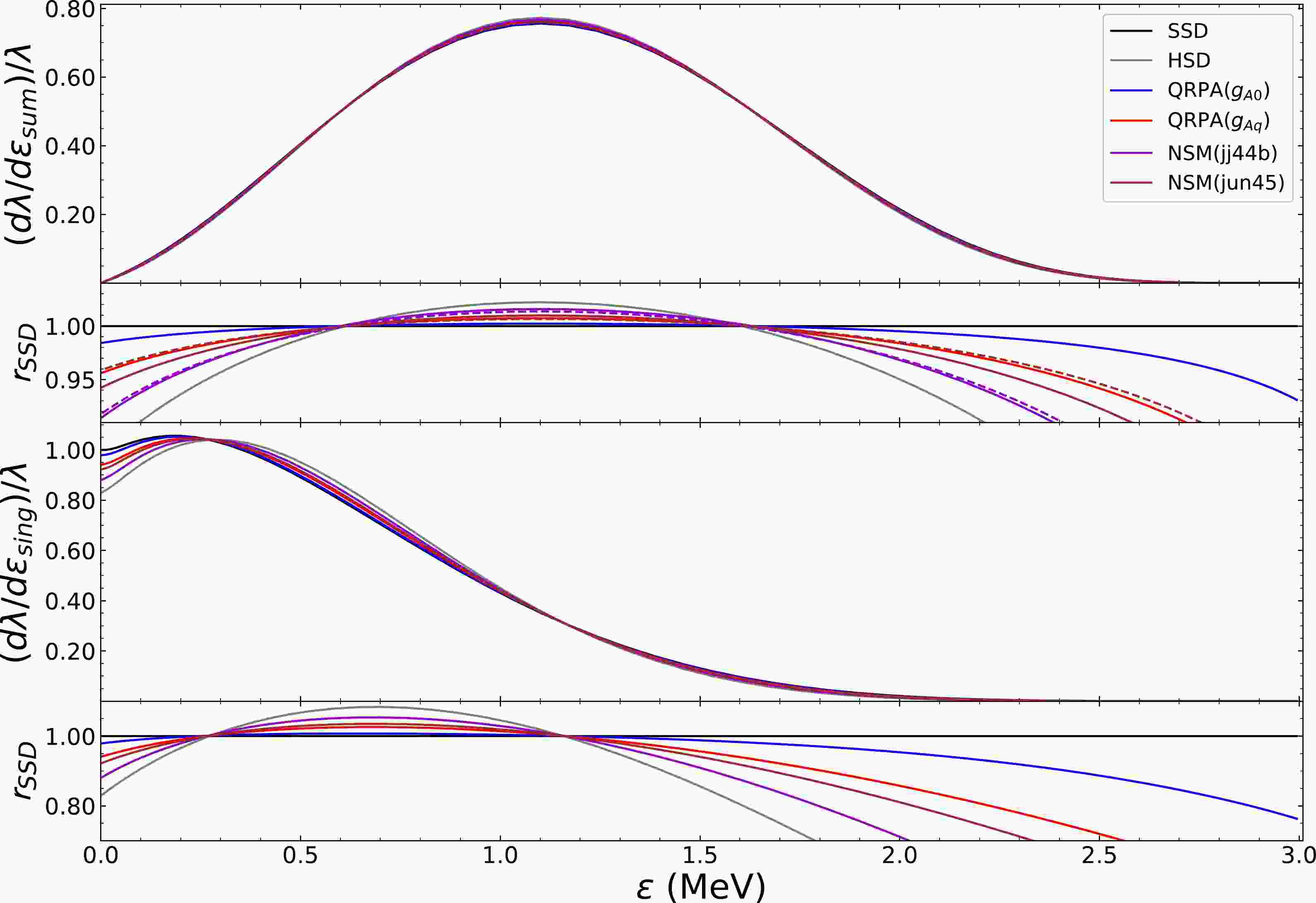
$ \chi^2/ $ ndf = 12.34/16 compared to HSD with$ \chi^2 $ /ndf = 35.32/16 for the single electron spectrum. Here, SSD and HSD are languages from the naive description of spectra from the roughest approximation (Eq. (13)). Our results for this nucleus are presented in Fig. 1, which suggests at first glance that the result without$ g_A $ quenching (blue line) is much closer to SSD than the quenched case (red line) for QRPA. In general, QRPA favors SSD over HSD. Meanwhile, for NSM calculations (bold lines),$ jj44b $ (Purple line) strongly favors HSD, and$ jun45 $ (brown line) lies in between the$ jj44b $ and QRPA results.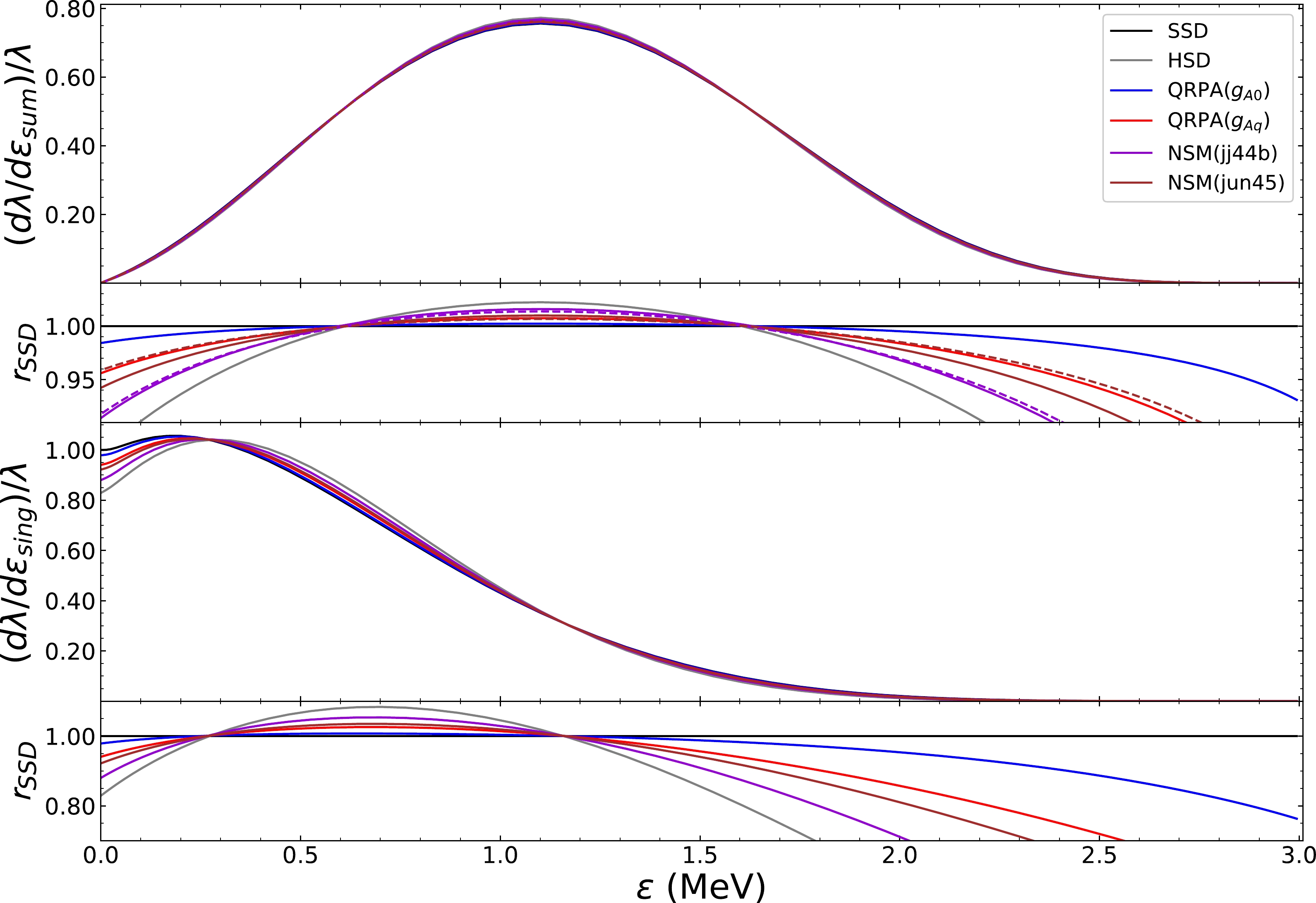
Figure 1. (color online) The electron spectra from NSM and QRPA calculations for
$ ^{82} $ Se. NSM calculations are with two Hamiltonians as indicated in the text, while for QRPA, we consider two cases:$ g_{A0} $ without$ g_A $ quenching and$ g_{Aq} $ with$ g_A=0.75g_{A0} $ . The dashed lines for NSM calculations are for the case considering only the first few states accumulating enough strength (see the text and also Fig. 3). The first and third panels represent the summed and single electron spectra, respectively, while the second and fourth panels represent ratios of each case over the spectra obtained from SSD hypothesis.Before proceeding to the detailed discussion of the spectra for this nucleus, we first use this nucleus as an example to show how the different intermediate states shape the electron spectra, to learn if it is possible to understand the spectra with the running sum from the intermediate states of double beta decay. In Fig. 2, we plot a comparison of spectra including only specific states (in this study, we categorize the states into low-, medium-, and high-lying states) to understand how different states contribute to the final spectra.
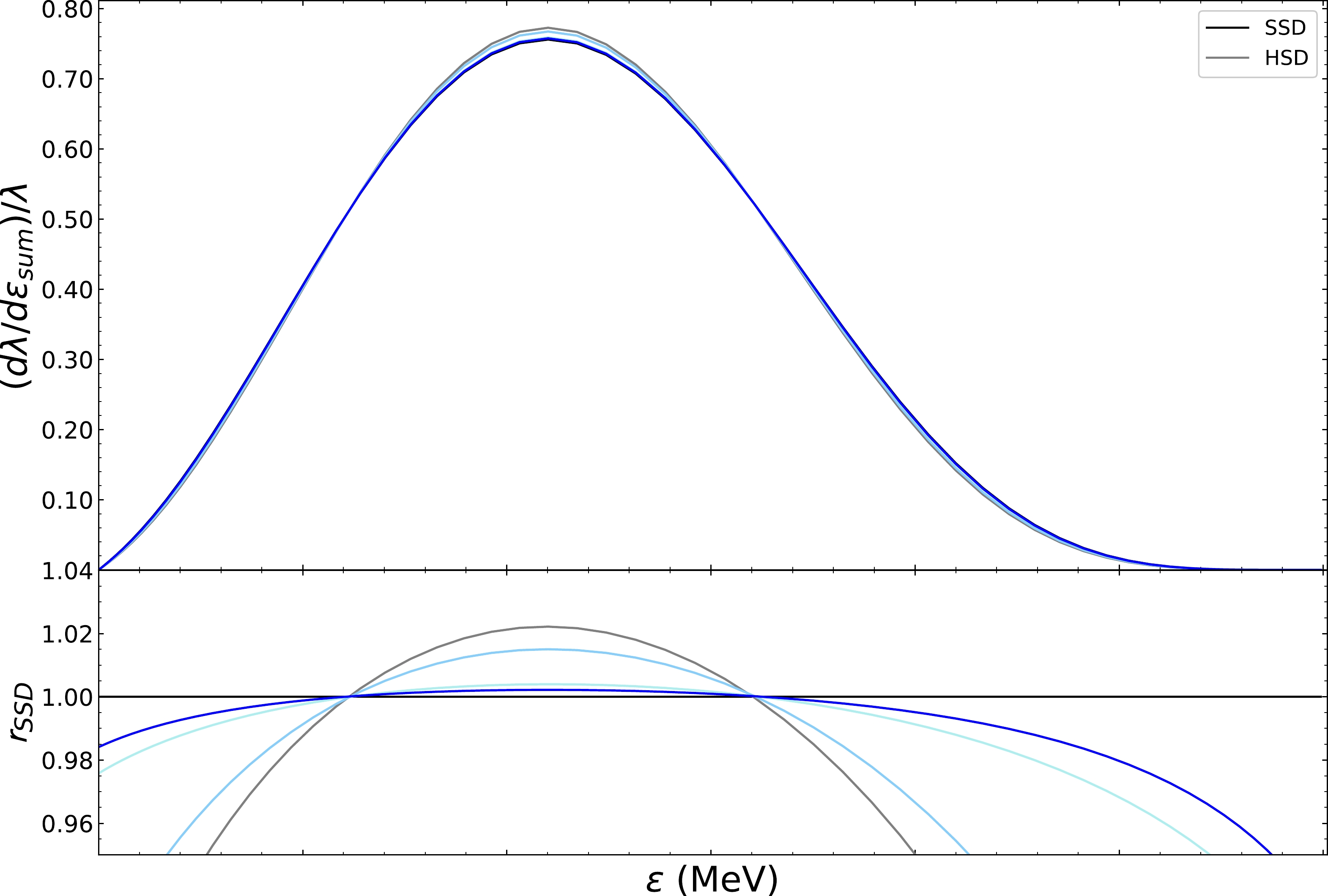
Figure 2. (color online) Illustration of how different states contribute to the summed spectra from QRPA calculations. The colors correspond to those in Fig. 3; the blue lines represent all intermediate states considered, while the light blue refers to the exclusion of high-lying states leading to the cancellation. Meanwhile, the pale blue curves represent low-lying states that accumulate enough strength to reproduce the half-life (see also Fig. 3). Here, the upper panel represents the spectra, and the lower panel with the
$ r_{SSD} $ label refers to the ratio of different normalized spectra divided by the normalized SSD spectrum.To explain the choices of the states included for each curve in Fig. 2, we first look at the running sum of the NMEs, which is a very good tool to understand the contributions of each state to the NME. As presented in literature [21, 22, 26], for QRPA, the running sum is crucial for understanding the nuclear structure issues in the double beta transition. It is with the SSD or low-lying state dominance (LSD) characteristics for the current nucleus, that is, the low- and medium-lying states accumulate enough strength much larger than the final strength and it is then cancelled by high-lying states, as shown in Fig. 3(blue and red lines). In this sense, just the low-lying states are already enough to describe the decay strength (running sum). For the running sum of NMEs in the current calculation, we find cancellations from states around excitation energies of 7 MeV, whose energies are slightly smaller than the GTR energy. The cancellations most likely result from a pygmy GTR; the cancellations from the giant GTR can be identified in the running sum around excitation energies of 12 MeV. However, their contributions are suppressed by the energy denominator. This is actually well understood for QRPA calculations. Therefore, for the next step, we want to study whether the spectra behave like NMEs, that is, the low-lying states alone determine the spectra if there are cancellations present. In other words, could the spectra indicate the cancellation information directly?
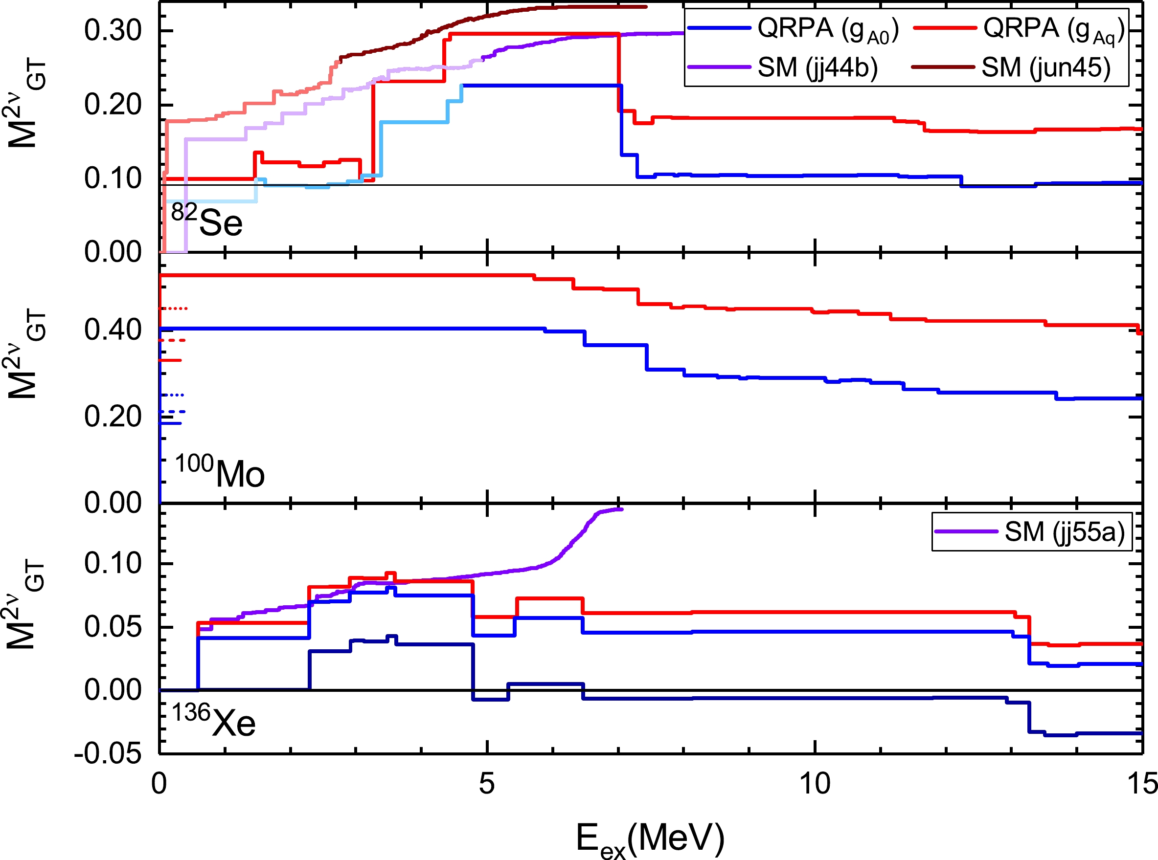
Figure 3. (color online) Running sum of
$M^{2\nu}_{\rm GT}$ for$ ^{82} $ Se,$ ^{100} $ Mo, and$ ^{136} $ Xe. For$ ^{82} $ Se, the QRPA and NSM results are presented, and different colors for QRPA without$ g_A $ quenching are explained in the text, so that for NSM. For$ ^{100} $ Mo, QRPA results are presented. The short horizontal lines refers to the experimental results from [8, 23] assuming SSD. For$ ^{136} $ Xe, we have an extra dark blue line for QRPA, which is explained in the text.To do this, we divide the intermediate states into three parts in Fig. 3 (we consider the case of QRPA calculations without quenching, represented by the blue serial lines): the low-lying states which already accumulate enough strength equal to the total final strength (the pale blue line), the additive low-lying (medium-lying) states which accumulate more strength reaching the maximum strength (the light blue line) and the third part is the cancellation to the excess strength from the high-lying states (the blue line). Correspondingly, in Fig. 2, we study the contributions of these three parts by comparing the spectra with the pale blue, light blue, and blue curves (the counterparts of the three pars in Fig. 3), respectively. In this way, we try to understand how the additive part and the cancellation part contribute to the spectra. The results are similar to that of NME, while spectra from the low-lying part are close to SSD shape, the additive part will push the spectra away from SSD shape to the HSD shape and the cancellations parts(high-lying states) will pull the spectra back. Moreover, the spectra are almost solely determined by the low-lying part which also accumulates enough strength for the running sum in Fig. 3 (both in pale light curves). This agrees with the conclusion in [1], which suggests that the spectra are sensitive to
$M^{2\nu}_{\rm GT-3}$ dominated by the low energy contribution. Therefore, if the contributions from the medium energy and high energy regions cancel each other (in our case, the light blue and blue curves), we barely see any implications in the spectra; that means, like the NME, the electron spectra cannot help us distinguish between the true single or low-lying state dominance (no strength from high-lying states) and effective SSD (LSD) (strength from high-lying states get cancelled by each other). Here, the analysis applies to the normal case. For special cases, such as the first state contributing more strength than needed or flipping the sign of the strength, the spectra will behave differently. Coincidentally, these are the cases for the other two nuclei that we are interested in; therefore, we leave these cases to subsequent sections.Now, we proceed to the discussion of the electron spectra from QRPA calculations, which are presented in Fig. 1. The spectra from QRPA seem to agree with the measurement, especially for a bare
$ g_A $ . Although the deviations from the head and tail seem drastic, they contribute less to the counts of the events. In general, the current QRPA calculation qualitatively reproduces the experimental results, and a cancellation from the high-lying states is expected in the current calculation. Future measurements will pin down the errors and give quantitative results, such as that for$ ^{136} $ Xe (which we will discuss later). These will help us better constrain the QRPA calculations since different calculations are still differentiated by details.Next, we apply such analysis to the NSM calculations as well. As we may be aware, simultaneous fulfillment of the GT strength of the parent and daughter nuclei to the intermediate nuclei and double beta decay strength for QRPA calculations has long been a problem [9]. This may be because we mimic the multi-phonon behavior by overestimating the particle-particle correlations, and this over-estimation for different observables is most probably different. This is also why, in this study, we do not analyze the B(GT) strength of the intermediate states to the parent and daughter nuclei from QRPA calculations. This will not be the case for the NSM calculation since all excitations beyond the one-phonon excitation are included. However, the NSM may face the problem of missing giant GTR (or the Pygmy one) strength, which serves as an important source of high energy cancellations to the double beta decay NME, as predicted from QRPA calculations. Also, for the low-lying states, some quenching is needed to account for the missing correlations outside the model space. The usual way to fix the quenching of
$ g_A $ for the$ 2\nu\beta\beta $ -decay is by fitting the$ 2\nu\beta\beta $ -decay NME [10]. In our current calculation, we fit the half-lives instead and find that the$ g_A $ is basically the same as that of fitting the NME. Our fitted$ g_A\sim 0.55 $ is slightly larger than the fitted value for$ ^{76} $ Ge [10] with a strength-function method. Also, one observes that the NME or half-life nearly converges with the current chosen number of intermediate states, this agree with various NSM calculations [27, 28]. However, with such a fitting strategy, despite the successful prediction of half-lives, the calculated spectra are not satisfactory. In Fig. 1, both NSM calculations (purple and brown solid lines) favor HSD and contradict current experimental data.Conversely, for
$ ^{82} $ Se, the charge exchange experiments$ ^{82} $ Se($ ^{3} $ He,t)$ ^{82} $ Br [24] offer relatively precise B(GT) values for the$ \beta^- $ side while the data for the$ \beta^+ $ side is still missing (see Fig. 4). To reproduce the experimental data of the low-lying strength from the NSM calculations, we find that a quenched value of$ q\equiv g_A/g_{A0}=0.6 $ is needed. However, we find that such a fitting for${{jun45}}$ , will lead to a large deviation for states with excitation energy larger than 5 MeV. A stronger quenching will cause better agreement for these high-lying states; however, the low-lying strength will be heavily suppressed. As we will show, the spectra impose severe constraints on the decay strength at a low excitation energy, and a larger quenching value is therefore needed. Nevertheless, these fitted$ g_A $ values are different from those of double beta decay.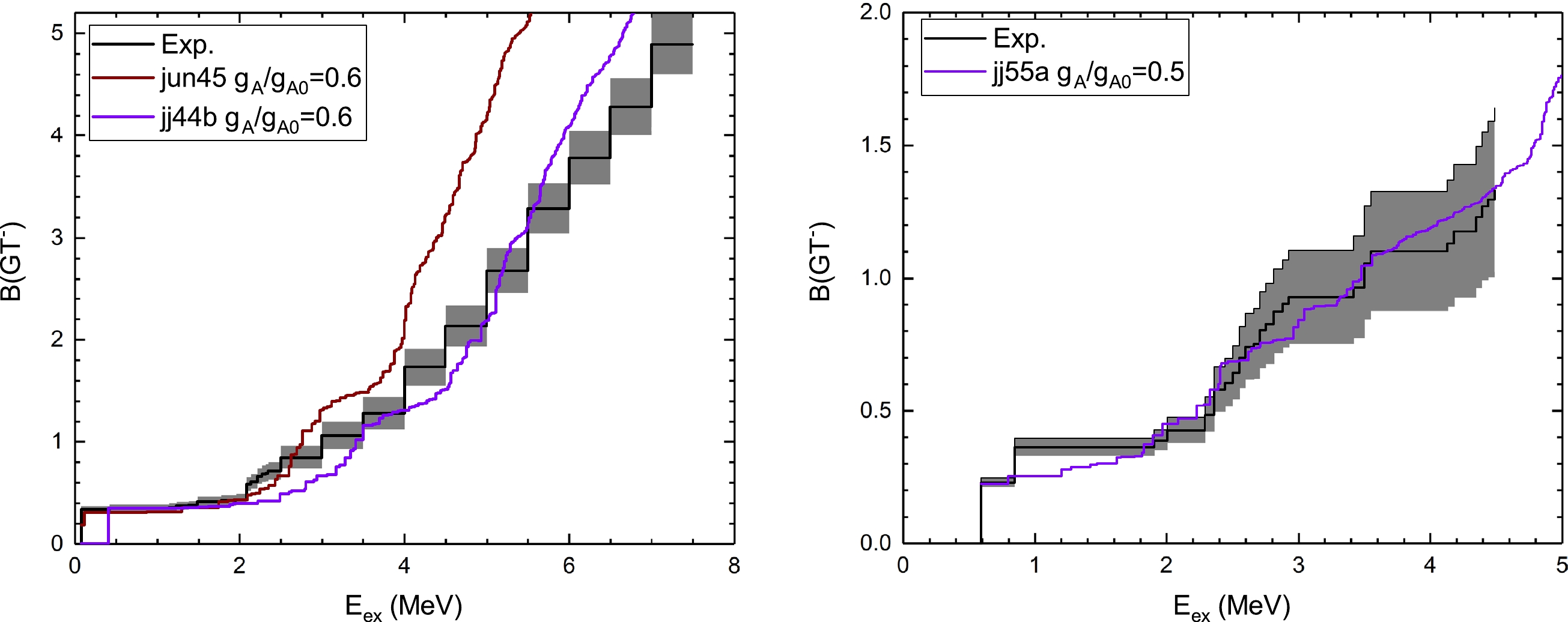
These discrepancies lead to severe reliability problems in the NSM description of double beta decay. A straightforward solution is that we adopt the same
$ g_A $ quenching for both charge-exchange reactions and double beta decay. With the fitted$ g_A $ from charge-exchange reactions, in the NSM calculations, the first few states accumulate enough strength to reproduce the decay strength (light brown and light purple lines in Fig. 3). From the above analysis, we then need to consider these low-lying states only for the spectra. We find that the new spectra are improved (dashed lines in Fig. 1), especially for results from${{jun45}}$ (dashed brown lines). These results also show that, for an SSD-like spectra, the results are extremely sensitive to the very low-lying states, and better agreement is achieved by${{jun45}}$ just because its first two states reproduce the experimental B(GT) in Fig. 4 better, despite the unsatisfactory description of B(GT) from higher-lying states. In this sense, these kinds of spectra can well constrain the strength distribution. The${{jj44b}}$ Hamiltonian is a bad example as it fails to reproduce the low-lying strength, just several hundred keV deviation of the excitation energy leads to a worse prediction. While the spectra imply high-lying cancellation from NSM calculations, we will not get this from NSM calculation even if we perform a full diagonalization of the NSM Hamiltonian. This is due to the lack of the spin-orbit partner of$ f_{7/2} $ and$ g_{9/2} $ .The current NSM results with proper treatment validate the simultaneous fulfillment of quenching for both β and
$ \beta\beta $ side and could predict things which are missing in the calculations. Nevertheless, we lack$ ^{82} $ Kr charge exchange data to establish a firm conclusion, and current study can be a good Ansatz for combined analysis on double beta decay and charge exchange reactions.Thus, the observed spectra rule out the NSM calculations with
${{jj44b}}$ Hamiltonian, although it gives a better agreement for low-lying B(GT). This suggests that the electron spectra can constrain the decay strength of the very low-lying states for the SSD case. Future measurements with a parametrized shape (see discussion in subsequent sections) could help us with a more quantitative analysis. -
The numerical estimation of electron spectra for
$ ^{100} $ Mo has been performed using Skyme meanfield based QRPA [8]. However, their prediction of the HSD trend has now been ruled out by NEMO-3 experiments. Our results differ greatly from theirs with a strong favor going beyond SSD. From Fig. 5, we find that for fitted$ g_{pp}^{T=0} $ in the$ g_{A0} $ and$ 0.75g_{A0} $ cases, the first state contributes more strength than the final decay strength requiring the cancellations from high-lying states. Compared to$ ^{82} $ Se, the cancellations from GTR and other states are somehow weakened. Nevertheless, we can still find traces of cancellation from pygmy or giant GTR from Fig. 3. As we have mentioned above, it is nearly impossible to simultaneously reproduce the following three quantities in QRPA calculation: B(GT$ ^- $ ), B(GT$ ^{+} $ ), and$M^{2\nu}_{\rm GT}$ [9]. However, with enlarged$ g_{pp} $ , we could always mimic the multi-phonon behavior for$M^{2\nu}_{\rm GT}$ . Since the ground state of$ ^{100} $ Tc comes out to be$ 1^+ $ , we could estimate the$ 2\nu\beta\beta $ -decay strength for the very first excited states from measurements. The analysis in [8] suggests that, with EC or charge-exchange reaction extracted B(GT$ ^- $ ) and β-decay extracted B(GT$ ^+ $ ) of$ ^{100} $ Tc, the NME from the first state, which is smaller than the final$ 2\nu\beta\beta $ NME, is given. Nevertheless, later analysis with the improved B(GT$ ^- $ ) from EC of$ ^{100} $ Tc [23] suggests that the first$ 1^+ $ state contributes an NME larger than the total$M^{2\nu}_{\rm GT}$ [29]. This agrees with our current calculations despite QRPA reproducing an even larger NME value from the first$ 1^+ $ excited state, as presented in Fig. 3 (the horizontal short lines at the y axis are the estimated NMEs from the first$ 1^+ $ state from various measurements). Our calculations for NMEs from the first$ 1^+ $ state agree with the analysis in [23] but differ by about 10% for both cases with or without$ g_A $ quenching.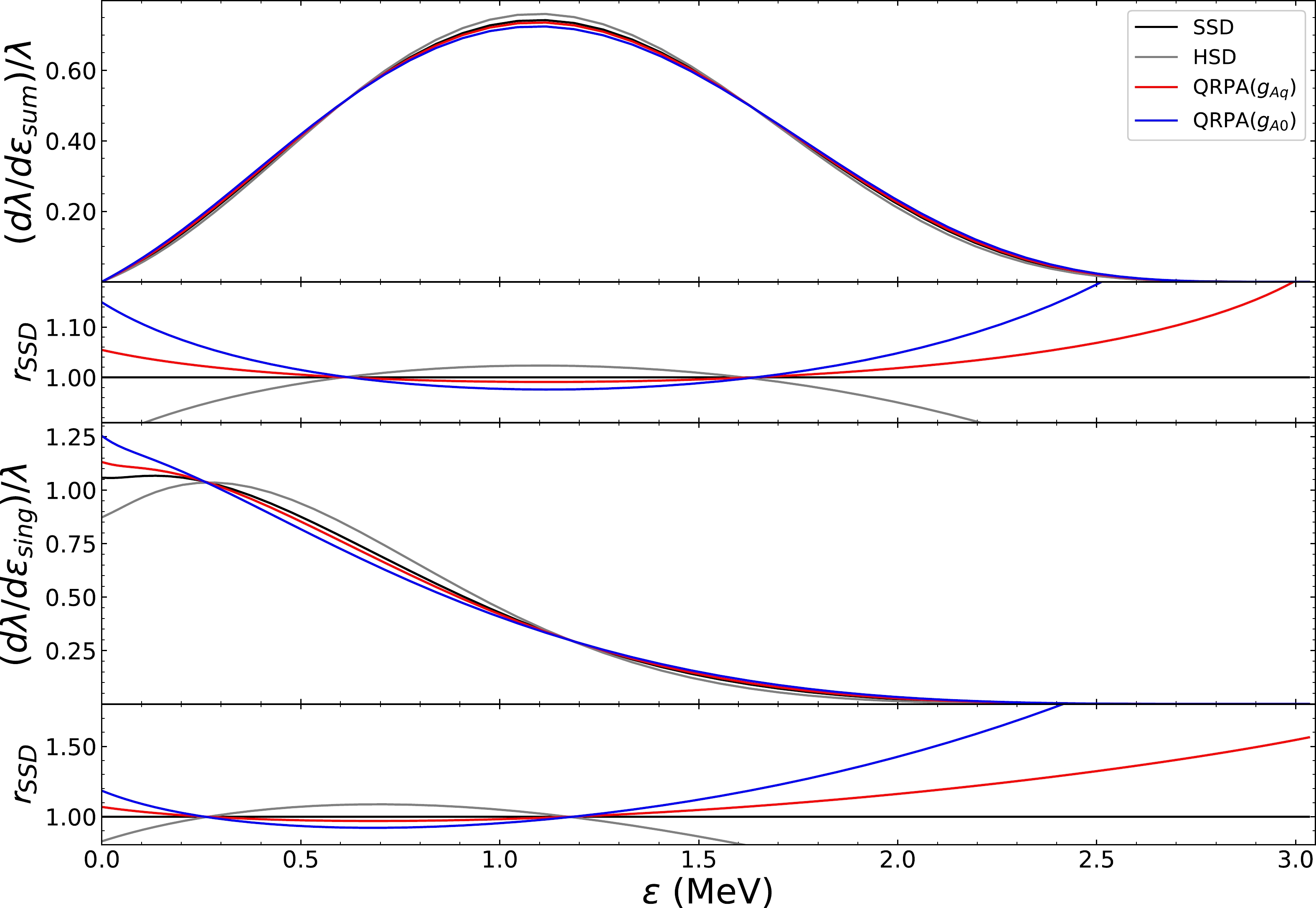
Figure 5. (color online) QRPA calculations of electron spectra for
$ ^{100} $ Mo. Here,$ g_{A0} $ means results without quenching, while$ g_{Aq} $ refers to the case of$ g_A=0.75g_{A0} $ .Such running sum behavior leads to visible effects on the electron spectra in Fig. 5. Unlike the case of
$ ^{82} $ Se, the predicted spectra do not lie in the region between SSD and HSD as one would expect in traditional PSF+NME treatment (Eq. (13)). The calculated spectra go beyond SSD. This means we will have more events at the spectra head or tail and fewer events around the peak for the summed spectra. This explicitly pointed out the inadequacy of the traditional expression from Eq. (13). For single electron spectra, they also look differently; more events will be observed at small and large electron energies and less for the medium electron energy range. These features have probably been observed in [6] with a simplified calculation (the SSD-3 model in [23, 30]), and current results actually agree well with the spectra obtained by NEMO experiments, where SSD preference is observed with$ \chi^2 $ /ndf = 1.54 compared to$ \chi^2/ $ ndf = 42.91 from HSD for a single electron spectrum. Notably, a delicate analysis shows that a simplified SSD-3 model has$ \chi^2/ $ ndf = 1.13, which is much smaller than that of a simple SSD model,$ \chi^2/ $ ndf = 1.45, for the summed electron spectra. However, the experiments slightly favor SSD for the single electron spectra. This confirms the existence of cancellations to the decay strength from states rather than the first one. However, we are still uncertain about the details of the cancellations.Therefore, measuring precise spectra could provide a solution to understanding these details. Also, if the B(GT
$ ^{+} $ ) and B(GT$ ^- $ ) strengths of the GTRs to the parent and daughter nuclei are measured once, we can surely get an idea of whether a cancellation from GTR should be present and the roles of other excited states. We will have a clear signature from the electron spectra for the case beyond SSD. Certainly, for this case, the cancellation must be happening, and by measuring the respective Gamow-Teller strength from GTR, we could get a general idea of whether a high-lying state cancellation exists, as predicted by most QRPA calculations [23]. Generally, for$ ^{100} $ Mo, electron spectra can be used to constrain the various QRPA calculations and rule out certain versions that fail to give a reasonable running sum of NME. -
The Taylor expansion method (TEM) prescription in [1] (Eq. (15)) actually provides very good parametrization for the electron spectra. As indicated by the phase space factor calculations [12], the spectra, like the phase space factor
$ G^{2\nu}(\tilde{A}) $ , converges with$\tilde{A}\ge E_{\rm GTR}$ . Here,$ \tilde{A} $ is the energy gap between the first$ 1^+ $ intermediate state and the ground states of the parent and daughter nuclei. One could easily observe that the 0th order PSF$ G^{2\nu}_0 $ in [1] is equivalent to traditional PSF at intermediate energy$ \tilde{A}\rightarrow \infty $ or the spectra of HSD. This suggests that the$ \xi^{2\nu}_{31}=0 $ case for TEM is actually HSD for traditional treatment. The traditional treatment of PSF covers the parameter space of$ \xi^{2\nu}_{31} $ from 0 to a finite positive value, corresponding to the positive energy gaps$ \tilde{A} $ from infinity to$ E_{1} $ defined after Eq. (5). As we have seen in$ ^{100} $ Mo, the actual spectra may not be restricted in this parameter space. Current data from KamLAND-Zen tends to give a small positive or even negative$ \xi^{2\nu}_{31} $ . This contradicts certain many-body approaches. In Fig. 3 of [2], one finds that both methods have been excluded at 1σ, and part of the QRPA parameter space has been excluded at the 2σ level.Our current QRPA calculation agrees with previous ones in [2], which somehow fails to reproduce the measured spectra. In this sense, a wrong prediction of cancellations is presented. Actually, in Fig. 6, the difference between the full numerical method (solid lines with corresponding colors) and that of TEM (dashed lines with corresponding colors) is illustrated. We find that the TEM has the same trend as full numerical calculations but deviates in detail. The deviation becomes more pronounced when the actual spectra are further away from the HSD case (for the current nucleus, unlike the previous two, we compare the spectra with those of HSD because they correspond to
$ \xi^{2\nu}_{31}=0 $ , close to the measured values). The comparison shows that, with the missing higher order correction such as$ \xi^{2\nu}_{51} $ [1], the TEM will underestimate the shift from HSD. Therefore, reproducing the required spectra already observed is difficult using the current QRPA calculations with the proper quenching factor.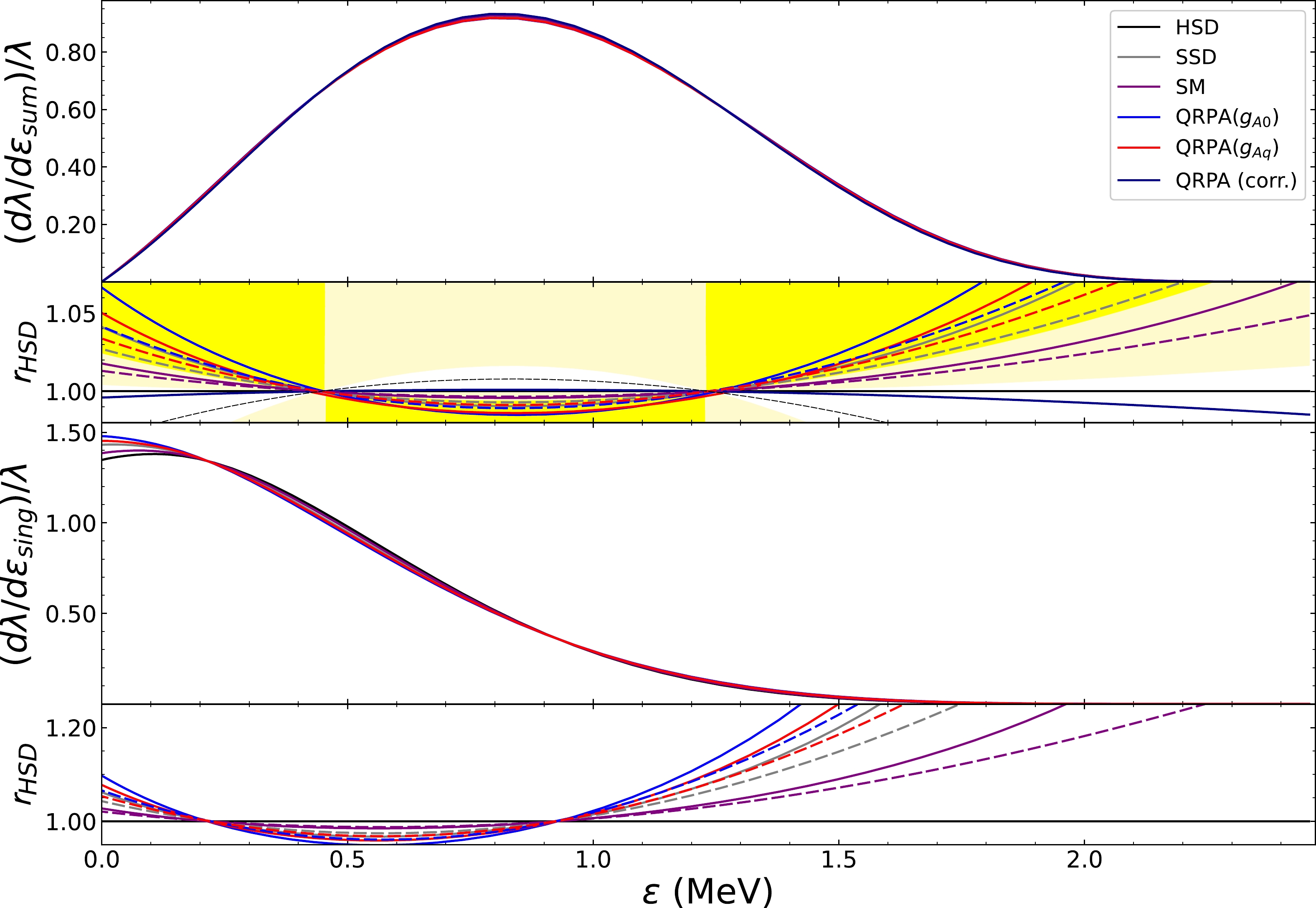
Figure 6. (color online) NSM and QRPA calculations of electron spectra for
$ ^{136} $ Xe. The ratios$r_{\rm HSD}$ here refer to the spectra relative to the HSD shape. Here, the legend (QRPA(corr.)) of dark blue lines refer to one fit of the NME by the negative values illustrated in Fig. 3. The dashed black line in the second graph represents the central value of the measured$ \xi_{31}^{2\nu} $ . The yellow and pale yellow regions in the second graph refer to the regions excluded at 90% and 68% C.L. by KamLAND-Zen [2]. The dashed lines here correspond to the results obtained with TEM (see text).The situation for the NSM is similar, with very strong
$ g_A $ quenching ($ g_A=0.4 $ ) applied in order to reproduce the experimental half-life. The prediction from${{jj55a}}$ has a strong low-lying strength and the calculated spectra lie in between HSD and SSD but are somehow excluded by a C.L. of 60%. Following the analysis in the above sections for$ ^{82} $ Se, from Fig. 4, we get$ g_A=0.5 g_{A0} $ by fitting the calculated running sum of B(GT) with experiments. In Fig. 4, our calculation basically reproduces the first GT and low-lying strengths up to excitation energies of 5 MeV. Unfortunately, no measurements are available for the$ \beta^+ $ side of$ ^{136} $ Ba to further validate our current choice. However, this choice of$ g_A $ will enhance the low-lying dominance characteristic and worsen the situation with the shift of spectra to the SSD side.The above analysis seems to announce the failure of both the QRPA and NSM calculations for predicting the electron spectra and rules out a strong cancellation, most probably from GTR, as observed for the two previous nuclei. However, the measurement still leaves us space since the central value of the measured spectrum shape parameter
$ \xi^{2\nu}_{31} $ lies in the negative region. Therefore, in the subsequent part, we explore another probability that helps us to reproduce the spectra in both the QRPA and NSM calculations. Of course, this new explanation needs more precise spectra measurements to pin down the errors. It only holds in the case of a negative$ \xi^{2\nu}_{31} $ .We start from QRPA calculation. For decades, the fitting of the parameter
$ g_{pp}^{T=0} $ (early days$ g_{pp} $ for both T=0 and T=1) relied on the$ 2\nu\beta\beta $ -decay GT NME. For these calculations, one begins with a curve starting at$ g_{pp}^{T=0}=0 $ (See, for example, Fig. 1 of [22]). Since there is an arbitrariness in the choice of the phase for the NME, one always sets the values at$ g_{pp}^{T=0}=0 $ to be positive, and then by default, one chooses the$ g_{pp}^{T=0} $ value to obtain a positive NME close to experimental one. The general reason for such a strategy could be for the approximate SU(4) symmetry [31], which requires a vanishing$M_{{\rm GT}-cl}^{2\nu}$ , and subsequently, a positive$M^{2\nu}_{\rm GT}$ . The negative NME is supposed to be unnatural despite not having collapsed yet for the QRPA equations. However, experimental evidence indicating the extent to which such symmetry is exact is still lacking. If we temporarily loosen this restriction, another possibility actually exists, which is that the fixed NME has a different sign from the value at$ g_{pp}^{T=0}=0 $ . For the running sum, this means the running sum flips its sign when the excitation energy increases, i.e., the high-lying GTR states will drag the strength from positive to negative. Our study suggests there is a small window for$ g_{pp}^{T=0} $ , in which the strength of first state has a different sign from the final strength (dark blue lines in Fig. 6), leading to a negative$ \xi^{2\nu}_{31} $ for TEM. The current measurement actually leaves a very narrow window for a positive$ \xi_{31}^{2\nu} $ and a large parameter space for a negative$ \xi_{31}^{2\nu} $ (see the unshaded region in the second panel of Fig. 6). This implies that a negative NME may be experimentally allowed, which could only be described by the current treatment or TEM.The calculated spectra with a flipped-sign running
$ M^{2\nu}_GT $ strength distribution are presented in Fig. 6(dark blue line). We find that the calculated spectra go beyond the HSD pattern, and the results agree well with the KamLAND-Zen measurement. The spectra lie close to the pattern of the obtained central value for the$ \xi^{2\nu}_{31} $ measurement. This implies that for future measurements, a negative$ \xi^{2\nu}_{31} $ strongly indicates a strong cancellation most probably from GTR flipping the sign of the running sum. In this sense, the cancellation confirmed by the two previous nuclei exists also for$ ^{136} $ Xe. Then, for NSM, the current data also suggest high-lying state cancellation to the decay strength. The discrepancy between the quenched$ g_A $ values from the$ 2\nu\beta\beta $ -decay strength and charge exchange reaction also disappears. Thus, we will need a decay strength cancellation of around 0.064 to reproduce the desired decay strength. Measurements of future charge exchange reactions will confirm our conclusion.Based on the above analysis, future reduction of uncertainty for the spectra measurement combined with charge exchange experiments will definitely give us more hints into the solutions for the current discrepancy. In this sense, these spectra can be used to constrain the many-body calculations. If the final measurement of parameter
$ \xi_{31}^{2\nu} $ is positive near 0, the current QRPA calculation fails to predict the low-lying strength for$ 2\nu\beta\beta $ -decay, as does the NSM calculation. These calculations could then be ruled out. Meanwhile, if$ \xi_{31}^{2\nu} $ is negative, the current QRPA calculations can reproduce the results, and a large reduction at high-lying states from the NSM is our major prediction for this nucleus. -
The
$ 2\nu\beta\beta $ -decay spectra offer us rich information and could be used to constrain nuclear structure calculations. Using the numerical treatment by combining with the charge exchange experiment data, we arrived at several important conclusions: i) the excitation states of the intermediate nuclei, which sum up enough strength to reproduce the experimental decay half-lives determine the spectra, and other high-lying states whose decay strength cancel each other do not contribute to the spectra; ii) this ensures a consistent description of the quenching factor for shell model calculations for$ ^{82} $ Se; and iii) both the shell model and QRPA calculations point to a reduction in high-lying states possibly from GTRs to the NME for the three nuclei concerned.The spectra can actually lie beyond the SSD and HSD shapes from the rough treatment; the former has been observed while the latter has never been considered, although there are traces from the KamLAND-Zen experiment. All our conclusions still need further verification with charge-exchange experiments, especially on the
$ \beta^+ $ side of the daughter nuclei. Further high precision double beta spectra measurements could help reduce the uncertainty of spectra shape. Together with the charge-exchange experiments, we could test the universality of high-lying state (possibly GTR) cancellations, which is common in QRPA calculations.
What can we learn from recent 2νββ experiments?
- Received Date: 2023-09-26
- Available Online: 2024-03-15
Abstract: Recent measurements of the two neutrino double beta decay high precision electron spectra, combined with charge exchange or β-decay experimental data, have revealed severe constraints across current nuclear many body calculations. Our calculations show that the quasi-particle random phase approximation (QRPA) approach can adequately reproduce the measured spectra for the two open shell nuclei,


 DownLoad: