-
The proposition of black hole thermodynamics has become a bridge connecting general relativity, classical thermodynamics, and quantum mechanics. With the establishment of the four laws of black hole thermodynamics, research on black hole thermodynamics and its thermodynamic properties has become one of the most interesting topics in theoretical physics [1−8]. Using the dual relation of AdS/CFT [9−11], the Hawking-Page phase transition can be interpreted as a confinement/deconfinement phase transition in the gauge field [12]. In 1984, Henneaux and Teitelboim proposed the cosmological constant of spacetime to be a dynamic variable [13−16]. In 2009, Kasto and Ray Tarschen took a significant step forward in their interpretation of the cosmological constant, taking it as the pressure of a black hole system [17], from which it was found that the first law of thermodynamics of AdS black holes is consistent with the Smarr relation. This opened a new era for the study of the thermodynamic properties of black holes in extended phase space. In the extended phase space, Kubiznak and Mann studied a small/large black hole phase transition and found that this transition is analogous to the liquid-gas transition of van der Waals systems [1]. Later, the study of the properties and phase structure of AdS black holes attracted attention [1−8]. Through research, it was found that AdS black holes have reentrant phase transitions, isolated critical points, and triple points [18−38].
In recent years, with extensive studies on dark energy and dark matter, the thermodynamic properties of de Sitter spacetime has attracted attention [2, 22, 39−55]. Recent astronomical observations show that approximately
$ 70 $ % of the energy density of the universe is composed of so-called dark energy. In general relativity, the cosmological term proposed by Einstein describes this type of dark energy matter. The analysis of supernova data also indicates that there is a positive cosmological constant in the universe. In the early inflationary period, our universe was a quasi de Sitter spacetime, and the cosmological constant term introduced in the study of de Sitter spacetime was the contribution of vacuum energy, which was also a form of material energy. If the cosmological constant corresponds to dark energy, our universe will evolve into a new de Sitter phase. The accelerated expansion of the universe shows that our universe is gradually becoming de Sitter. In addition, the success of AdS/CFT has prompted researchers to look for similar dual relations of de Sitter space; therefore, the study of de Sitter spacetime is not only of theoretical interest but also a practical necessity.The dS space attracts a high level of research interest because its corresponding cosmological model is potentially consistent with the observational results supporting the late-time accelerating expansion of the universe [56]. Despite this, thermodynamical phenomena in asymptotically dS black holes remain barely explored, whereas those in asymptotically AdS black holes have been substantially discovered. Theoretically, thermodynamical studies on Schwarzschild–de Sitter (Sch-dS) black holes have historically encountered a number of difficulties. Among the many issues hindering progress, the obscurities in dealing with the notion of mass and the thermodynamical consideration of a multihorizon system are two main problems. The former is due to the absence of a globally timelike Killing vector field, which prevents one from obtaining a well-defined asymptotic mass [22, 57−58]. The latter results from the fact that the black hole and cosmic horizons are generally different temperatures, such that the Sch-dS black hole as a multihorizon system is out of equilibrium.
As we all know, de Sitter spacetime has a black hole horizon and cosmological horizon, and both horizons have Hawking radiation with different temperatures. In general, the radiation temperatures and thermodynamic quantities of the two horizons are functions of parameters of the spacetime, and the thermodynamic quantities of the two horizons are not independent. This is a concern in theoretical physics when using one thermodynamic system to reflect the thermodynamic properties of spacetime [42−60]. For any physical system, the first law of thermodynamics should be met, which suggests that the construction of a system reflecting the thermodynamic properties of the entire de Sitter spacetime must meet the first law of thermodynamics. From this, the equivalent thermodynamic quantities of spherically symmetric charged spacetime are obtained by solving the equation [50, 51]. Therefore, the aim of this study is to investigate the equivalent thermodynamic quantities of five-dimensional de Sitter hairy spacetime and the thermodynamic properties of the spacetime described by these quantities.
This paper is arranged as follows. In Sec. II, the equivalent thermodynamic quantities of five-dimensional de Sitter hairy spacetime are given, and the laws of the Hawking radiation temperatures of the black hole event horizon and cosmic event horizon and the equivalent temperature of spacetime varying with the position ratio between the two event horizons under different parameters are discussed. In addition, another important relation to describe the thermodynamic properties of spacetime, the Smarr relation of five-dimensional de Sitter hairy spacetime, is obtained using the Eulerian function theorem. In Sec. III, the method of studying the phase transition of van de Waals systems or charged AdS black holes is extended to study five-dimensional de Sitter hairy spacetime. It is found that five-dimensional de Sitter hairy spacetime has a phase transition similar to that of van de Waals systems or charged AdS black holes. However, the constant volume heat capacity of five-dimensional de Sitter hairy spacetime described by the equivalent thermodynamic quantity is not zero, which is different from the case of AdS black holes but consistent with that of general thermodynamic systems. This shows that five-dimensional de Sitter hairy spacetime described by the equivalent thermodynamic quantity is more universal. In Sec. IV, using the Ehrenfest scheme, we testify that the critical behaviors belong to the second order phase transition. The conclusions are presented in Sec. V (we use the geometric units
$ G=\hbar=k_B=c=1 $ ). -
We begin our research in the context of Lovelock gravity minimally coupled to a Maxwell field. The scalar hair is conformally coupled to gravity via the dimensionally extended Euler densities in terms of the rank four tensor [41, 61−64],
$ \begin{equation} S_{\mu\nu} ^{\gamma\delta}=\phi^{2}R_{\mu\nu}^{\gamma\delta}-2\delta_{[\mu}^{[\gamma}\delta_{\nu]}^{\delta]} \nabla_{\rho}\phi\nabla^{\rho}\phi-4\phi\delta_{[\mu}^{[\lambda}\nabla_{\nu]}\nabla^{\delta]} \phi+8\delta_{[\mu}^{[\gamma}\nabla_{\nu]} \phi\nabla^{\delta]}\phi, \end{equation} $

(1) where ϕ is the scalar field. Under the conformal transformation,
$ g_{\mu\nu}\rightarrow \Omega^{2}g_{\mu\nu} $ and$ \phi\rightarrow \Omega^{-1}\phi $ as$ S_{\mu\nu}^{\gamma\delta}\rightarrow \Omega^{4}S_{\mu\nu}^{\gamma\delta} $ . The action for the theory in d spacetime dimensions is given by$ \begin{equation} I=\frac{1}{16\pi G}\int d^{d}x\sqrt{-g}\bigg(\sum\limits_{k=0}^{k_{\max}}L^{(k)}-4\pi GF_{\mu\nu}F^{\mu\nu}\bigg), \end{equation} $

(2) where
$ F_{\mu\nu}=\partial \mu A_{\nu}-\partial \nu A_{\mu} $ , and the Lagrangian densities are given by$ \begin{equation} L^{(k)}=\frac{1}{2^k}\delta^{(k)}\bigg(a_{k}\prod\limits_{r}^{k}R_{\mu_{r}\nu_{r}}^{\alpha_{r}\beta(r)}+b_{k}\phi^{d-4k}\prod\limits_{r}^{k}S_{\mu_{r}\nu_{r}}^{\alpha_{r}\beta(r)}\bigg), \end{equation} $

(3) where
$ a_{k} $ and$ b_{k} $ are coupling constants, and$ \delta^{(k)} $ is the generalized Kronecker tensor.Here, we are interested in spherically symmetric topological black hole solutions to this theory. In
$ 5 $ -dimensional spacetime, this metric is of the form$ \begin{equation} {\rm d} s^{2}=-f(r) {\rm d} t^{2}+f^{-1} {\rm d} r^{2}+r^{2} {\rm d} \Omega^{2}_{3}, \end{equation} $

(4) with the horizon function
$ \begin{equation} f(r)=1-\frac{8M}{3 \pi r^{2}}-\frac{\Lambda r^{2}}{6}-\frac{H}{r^{3}}+\frac{4 \pi Q^{2}}{3 r^{4}}, \end{equation} $

(5) where M, H, and Q are the black hole mass, hair parameter, and charge, respectively, and Λ is the cosmological constant. A black hole has three positive horizons: the black hole event horizon
$ r_{+} $ , internal (Cauchy) horizon$ r_{-} $ , and cosmological horizon$ r_{c} $ . From Eq. (5), we can obtain$ \begin{equation} M=\frac{3 \pi r_+^{2}}{8}-\frac{3 \pi \Lambda r_+^{4}}{48}-\frac{3 \pi H}{8 r_+}+\frac{ \pi^{2} Q^{2}}{2 r_+^{2}}, \end{equation} $

(6) $ \begin{equation} M=\frac{3 \pi r_{c}^{2}}{8}-\frac{3 \pi \Lambda r_{c}^{4}}{48}-\frac{3 \pi H}{8 r_{c}}+\frac{ \pi^{2} Q^{2}}{2 r_{c}^{2}}. \end{equation} $

(7) According to Eq. (5), we find that the Hawking radiation temperatures of the black hole horizon and cosmological horizon from
$ T_{+}=\dfrac{f^{\prime}(r_{+})}{4\pi} $ and$ T_{c}=-\dfrac{f^{\prime}(r_{c})}{4\pi} $ are$ \begin{equation} T_+=\frac{1}{2 \pi r_+}-\frac{\Lambda r_+}{6 \pi}-\frac{2 Q^{2}}{3 r_+^{5}}+\frac{H}{4 \pi r_+^{4}}, \end{equation} $

(8) $ \begin{equation} T_{c}=-\frac{1}{2 \pi r_{c}}+\frac{\Lambda r_{c}}{6 \pi}+\frac{2 Q^{2}}{3 r_{c}^{5}}-\frac{H}{4 \pi r_{c}^{4}}. \end{equation} $

(9) The thermodynamic quantities corresponding to the black hole event horizon satisfy the first law of thermodynamics and the Smarr relation,
$ \begin{equation} \begin{aligned} &\delta M=-T_+ \delta S_++V_+ \delta P+\phi_+ \delta Q+k_+ \delta H, \end{aligned} \end{equation} $

(10) $ \begin{equation} \begin{aligned} &2M=3 T_+ S_+-2 V_+ P+2 \phi_+ Q+3 k_+ H, \end{aligned} \end{equation} $

(11) where
$ \Lambda=-8 \pi P $ . The entropy, thermodynamic volume, and electric potential corresponding to the black hole horizon are$ \begin{equation} S_+ = \frac{\pi^{2} r_+^{3}}{2}, \quad V_+ = \frac{\pi^{2} r_+^{4}}{2}, \quad \phi_+ = \frac{\pi^{2} Q^{2}}{r_+^{2}}, \quad k_+ = -\frac{3 \pi}{8 r_+}. \end{equation} $

(12) The thermodynamic quantity corresponding to the cosmological horizon satisfies the first law of thermodynamics and the Smarr relation,
$ \begin{equation} \begin{aligned} &\delta M=-T_{c} \delta S_++V_{c} \delta P+\phi_{c} \delta Q+\kappa_{c} \delta H, \end{aligned} \end{equation} $

(13) $ \begin{equation} \begin{aligned} &2M=3 T_{c} S_+-2 V_{c} P+2 \phi_{c} Q+3 k_{c} H. \end{aligned} \end{equation} $

(14) The entropy, thermodynamic volume, and electric potential corresponding to the cosmological horizon are
$ \begin{equation} S_{c}=\frac{\pi^{2} r_{c}^{3}}{2}, \quad V_{c}=\frac{\pi^{2} r_{c}^{4}}{2}, \quad \phi_{c}=\frac{\pi^{2} Q^{2}}{r_{c}^{2}}, \quad k_{c}=-\frac{3 \pi}{8 r_{c}}. \end{equation} $

(15) From Eqs. (6) and (7), we can write the mass and cosmological constant of spacetime as
$ \begin{aligned}[b] M=&\frac{3 \pi r_{c}^{2}(1+x^2)}{16}-\frac{3 \pi \Lambda r_{c}^{4}(1+x^4)}{96}\\&-\frac{3 \pi H (1+x)}{16 r_{c} x}+\frac{\pi^2 Q^{2}(1+x^2)}{4 r_{c}^{2} x^2}, \end{aligned} $

(16) $ \begin{equation} \Lambda = \frac{6}{r_{c}^{2}(1+x^2)} - \frac{6 H}{x r_{c}^{5}(1+x^2)(1+x)} - \frac{8 \pi Q^2}{x^2 r_{c}^{6} (1+x^2)}, \end{equation} $

(17) where
$ x = r_{+}/r_{c} $ . From Eqs. (10) and (13), we know that the parameters$ M, Q, H $ , and Λ are the same in the two event horizons, whereas the entropy, temperature, thermodynamic volume, and electric potential corresponding to the two event horizons are different. Because the Hawking radiation temperatures of the two event horizons are generally different, if the thermodynamic systems corresponding to the two event horizons are studied separately, there are two independent thermodynamic systems with different temperatures in spacetime. Such considerations are obviously incomplete because$ M, Q, H $ , and Λ corresponding to the two event horizons are the same, and hence, the thermodynamics corresponding to the two event horizons in dS spacetime are interrelated and cannot be considered separately. The thermodynamic relations (10), (11), (13), and (14) cannot fully reflect the thermodynamic characteristics of dS spacetime; therefore, it is necessary to construct a relationship that can fully reflect the thermodynamics of dS spacetime, that is, the thermodynamic quantities of dS spacetime.It is well known that the first law of thermodynamics is a universal relation in thermodynamic systems. If the mass M, charge Q, and volume V in spacetime are taken as the state parameters of a thermodynamic system, these state parameters should meet the first law of thermodynamics,
$ \begin{equation} {\rm d}M=T_{\it{\rm{\rm{eff}}}} {\rm d}S-P_{\it{\rm{eff}}} {\rm d}V+\phi_{\it{\rm{eff}}} {\rm d}Q+k_{\it{\rm{eff}}} {\rm d}H, \end{equation} $

(18) and the thermodynamic volume of spacetime is [2]
$ \begin{equation} V=V_{c}-V_+=\frac{\pi^2 r_{c}^{4}}{2}(1-x^4), \end{equation} $

(19) and the total entropy of the system is
$ \begin{equation} S=S_++S_{c}+\bar{S}=\frac{\pi^2 r_{c}^{3}}{2}[1+x^{3}+f(x)]=\frac{\pi^2 r_{c}^{3}}{2} F(x), \end{equation} $

(20) with
$ x=r_{+}/r_{c} $ , and the term$ \dfrac{\pi^2 r_{c}^{3}}{2}f(x) $ is introduced owing to the interaction between the two horizons. From Eq. (18), we obtain$ \begin{aligned}[b]& T=\bigg(\frac{\partial M}{\partial S}\bigg)_{V,Q,H}\;, \quad P=\bigg(\frac{\partial M}{\partial V}\bigg)_{S,Q,H}\;, \\& \phi=\bigg(\frac{\partial M}{\partial Q}\bigg)_{S,V,H}\;, \quad k=\bigg(\frac{\partial M}{\partial H}\bigg)_{S,V,Q}\;. \end{aligned} $

(21) From Eqs. (16), (19), and (20), we can obtain the effective temperature of spacetime
$ \begin{aligned}[b] \it{T_{\rm{eff}}}=&\frac{3}{2 \pi r_{c} A(x)(1+x^2)}\Bigg\{\Bigg[x(1-x^2+x^4)\\&+\frac{H (1+x)(1+x^2)(1+x^5)-3x^4}{2 r_{c}^3 x^2 (1+x)}\Bigg]\\&-\frac{4 \pi Q^{2}[(1+x^2)(1+x^6)-x^4]}{3 r_{c}^4 x^3}\Bigg\}, \end{aligned} $

(22) and the effective pressure
$ \begin{aligned}[b]\\[-8pt] \it{P_{\rm{eff}}}=&\frac{3x}{8 \pi r_{c}^2 (1+x^2)A(x)}\Bigg\{3F(x)\Bigg[\frac{1}{1+x^2}\\&+\frac{1+2x+3x^2+4x^3}{2r_{c}^3x^3(1+x^2)(1+x)^2}-\frac{4\pi Q^2(1+2x^2)}{3r_{c}^4x^4(1+x^2)}\Bigg]-xF'(x)\\&\times\Bigg[1+\frac{1+x+x^2+x^3+x^4}{2r_{c}^3x^3(1+x)}-\frac{4\pi Q^2(1+x^2+x^4)}{3r_{c}^4x^4}\Bigg]\Bigg\}, \end{aligned} $

(23) where
$ A(x)=(1-x^4)F'(x)+3 x^3 F(x) $ , and the effective potential$ \it{\phi_{\rm{eff}}} $ and$ \it{k_{\rm{eff}}} $ are$ \begin{equation} \it{\phi_{\rm{eff}}}=\frac{\pi^2 Q (1+x^2)}{2r_+^{2}}, \quad k_{\rm{eff}}=-\frac{3 \pi (1+x)}{16r_+}. \end{equation} $

(24) When the Hawking temperature of the black hole event horizon is equal to that of the cosmological horizon, these temperatures are also equal to the effective temperature of spacetime, that is,
$ T_{+}=T_{c}=\it{T_{\rm{eff}}} $ ; based on Eqs. (8) and (9), when$ \begin{equation} \Lambda=\frac{3}{r_{c}^{2}x}+\frac{3H(1+x^4)}{2r_{c}^5x^4(1+x)}-\frac{4\pi Q^2(1+x^5)}{r_{c}^6x^5(1+x)}, \end{equation} $

(25) the Hawking temperature of the black hole horizon is equal to that of the cosmological horizon.
From Eqs. (17) and (25), we find that when the radiation temperatures of the two event horizons are equal, the charge Q, hair parameter H, cosmological horizon position
$ r_{c} $ , and position ratio x of the two event horizons satisfy$ \begin{aligned}[b] 0=&\frac{3}{r_{c}^{2}}+\frac{3H[(1+x+x^2)^2+x^2]}{2r_{c}^5x^3(1+x)}\\&-\frac{4\pi Q^2[(1+x+x^2)(1+x^2)+x^2]}{r_{c}^6x^4}, \end{aligned} $

(26) and from Eqs. (8), (9), (25), and (26), it is known that the radiation temperature is
$ \begin{aligned}[b] T=&T_{c}=T_+=\bigg[1+\frac{H(2+x+2x^2)}{2r_{c}^3 x (1+x)^3}\bigg]\\&\times \frac{(1-x^4)(1+x)}{2\pi r_{c}(1+x^2)[(1+x+x^2)(1+x^2)+x^2]}. \end{aligned} $

(27) Substituting Eq. (27) into Eq. (22), we obtain
$ \begin{aligned}[b] \it{T_{\rm{eff}}}=&\frac{3x^2(1+x)(1+x^5)}{2\pi r_{c}(1+x^2)[(1+x+x^2)(1+x^2)+x^2]}\\&\times \frac{1}{\left[(1-x^4)F'(x)+3x^3F(x)\right]}\times\left[1+\frac{H(2+x+2x^2)}{2r_{c}^3 x (1+x)^3}\right]. \end{aligned} $

(28) From
$ T=T_{c}=T_{+}=\it{T_{\rm{eff}}} $ , we can see that$ \begin{equation} A(x)=(1-x^4)F'(x)+3x^3F(x)=\frac{3x^2(1+x^5)}{1-x^4}, \end{equation} $

(29) and the solution of the above differential equation is
$ \begin{equation} F(x)=\frac{11}{7}(1-x^4)^{\frac{3}{4}}-\frac{4(1+x^7)-7x^3(1+x)}{7(1-x^4)}. \end{equation} $

(30) Substituting Eq. (29) into Eq. (22), we obtain the effective temperature
$ \begin{aligned}[b] \it{T_{\rm{eff}}}=&\frac{1-x^2}{2\pi x r_{c}(1+x^5)} \Bigg[1-x^2+x^4\\&+\frac{H[(1+x^5)(1+x)(1+x^2)-3x^4]}{2r_{c}^3 x^3(1+x)}\Bigg]\\&-\frac{4\pi Q^2[(1+x^2)(1+x^6)-x^4]}{3r_{c}^4 x^4}, \end{aligned} $

(31) and this effective temperature can be rewritten as
$ \begin{equation} \it{T_{\rm{eff}}}=\frac{f_{1}(x)}{r_{c}}+\frac{Hf_{2}(x)}{r_{c}^4}-\frac{Q^2 f_{3}(x)}{r_{c}^5}, \end{equation} $

(32) where
$ \begin{aligned}[b] &f_{1}(x)=\frac{(1-x^2)(1-x^2+x^4)}{2\pi x (1+x^5)},\\ &f_{2}(x)=\frac{(1-x)[(1+x^5)(1+x)(1+x^2)-3x^4]}{4\pi x^4(1+x^5)},\\ &f_{3}(x)=\frac{2(1-x^2)[(1+x^2)(1+x^6)-x^4]}{3 x^5 (1+x^5)}. \end{aligned} $

(33) Substituting Eq. (29) into Eq. (23), we obtain the effective pressure of spacetime
$ \begin{equation} \it{P_{\rm{eff}}}=\frac{1}{8\pi r_{c}^2}\left(f_{4}+\frac{Hf_{5}(x)}{r_{c}^3}-\frac{4\pi Q^2 f_{6}(x)}{r_{c}^4}\right), \end{equation} $

(34) where
$ \begin{aligned}[b] f_{4}(x)=&\frac{3F(x)(1-x^2)}{x(1+x^5)(1+x^2)}-\frac{(1-x^2)F'(x)}{1+x^5},\\ f_{5}(x)=&\frac{3F(x(1-x)(1+2x+3x^2+4x^3)}{2 x^4(1+x^5)(1+x^2)(1+x)}\\&-\frac{(1-x)(1+x+x^2+x^3+x^4)F'(x)}{2 x^3(1+x^5)},\\ f_{6}(x)=&\frac{F(x)(1-x^2)(1+2x^2)}{x^5 (1+x^5)(1+x^2)}-\frac{(1-x^2)(1+x^2+x^4)F'(x)}{3 x^4(1+x^5)}. \end{aligned} $

(35) The Smarr formula stands among the pillars of black hole thermodynamics, and extensive research over the past four decades [8, 17, 59, 60, 65−71] has revealed a strong relationship between gravitation, thermodynamics, and quantum theory.
Let the mass of the black hole be a homogeneous function of entropy, volume, charge, and the hair parameter, that is,
$ M=M(S, V, Q, H) $ , and for the five-dimensional case, let the units of the thermodynamic quantities be [17]$ \begin{equation} [M]=L^2, \quad [S]=L^3, \quad [H]=L^3, \quad [V]=L^4, \quad [Q]=L^2, \end{equation} $

(36) where L represents the units of length. According to the previous theorem, the mass satisfies
$ \begin{aligned}[b] 2M(S, V, Q, H)=&3 S \left(\frac{\partial M}{\partial S}\right)+4V\left(\frac{\partial M}{\partial V}\right)\\&+2Q\left(\frac{\partial M}{\partial Q}\right)+3H\left(\frac{\partial M}{\partial H}\right), \end{aligned}$

(37) and from Eq. (18), we obtain
$ \begin{aligned}[b] & \left(\frac{\partial M}{\partial S}\right)=\it{T_{\rm{eff}}}, \quad \left(\frac{\partial M}{\partial V}\right)=-\it{P_{\rm{eff}}}, \\& \left(\frac{\partial M}{\partial Q}\right)=\it{\phi_{\rm{eff}}}, \quad \left(\frac{\partial M}{\partial H}\right)=\it{k_{\rm{eff}}}. \end{aligned} $

(38) Substituting Eq. (38) into Eq.(37), we obtain the Smarr relation of spacetime
$ \begin{equation} \begin{aligned} 2M(S, V, Q, H)=&3S\it{T_{\rm{eff}}}-4VP_{\it{\rm{eff}}}+2Q\it{\phi_{\rm{eff}}}+3H\it{k_{\rm{eff}}}, \end{aligned} \end{equation} $

(39) from which we find that in charged de Sitter hairy spacetime, both the first law of thermodynamics and the Smarr relation contain
$ V\it{P_{\rm{eff}}} $ and$ H\it{\kappa_{\rm{eff}}} $ terms; therefore, only when the pressure and volume terms are included, the first law of thermodynamics of spacetime and the Smarr relation are self consistent.To understand the variation in the radiation temperature
$ T_{+} $ of the black hole event horizon, the radiation temperature$ T_{c} $ of the cosmological horizon, and the effective temperature$ \it{T_{\rm{eff}}} $ of spacetime with the position ratio x of the two event horizons, substituting Eq. (17) into Eq. (8) and Eq. (9), we obtain the radiation temperatures for the two event horizons,$ \begin{aligned}[b] T_+=&\frac{1-x}{2\pi x r_{c}(1+x^2)}\Bigg[1+x+\frac{H(1+2x+3x^2+4x^3)}{2r_{c}^3 x^3(1+x)}\\&-\frac{4\pi Q^2(1+x+x^2+x^3)}{3r_{c}^4 x^4}\Bigg], \end{aligned} $

(40) $ \begin{aligned}[b] T_{c}=&\frac{1-x}{2\pi r_{c}(1+x^2)}\Bigg[1+x+\frac{2H(4+3x+2x^2+x^3)}{r_{c}^3 x(1+x)}\\&-\frac{4\pi Q(1+x)(2+x^2)}{3r_{c}^4 x^2}\Bigg]. \end{aligned} $

(41) The
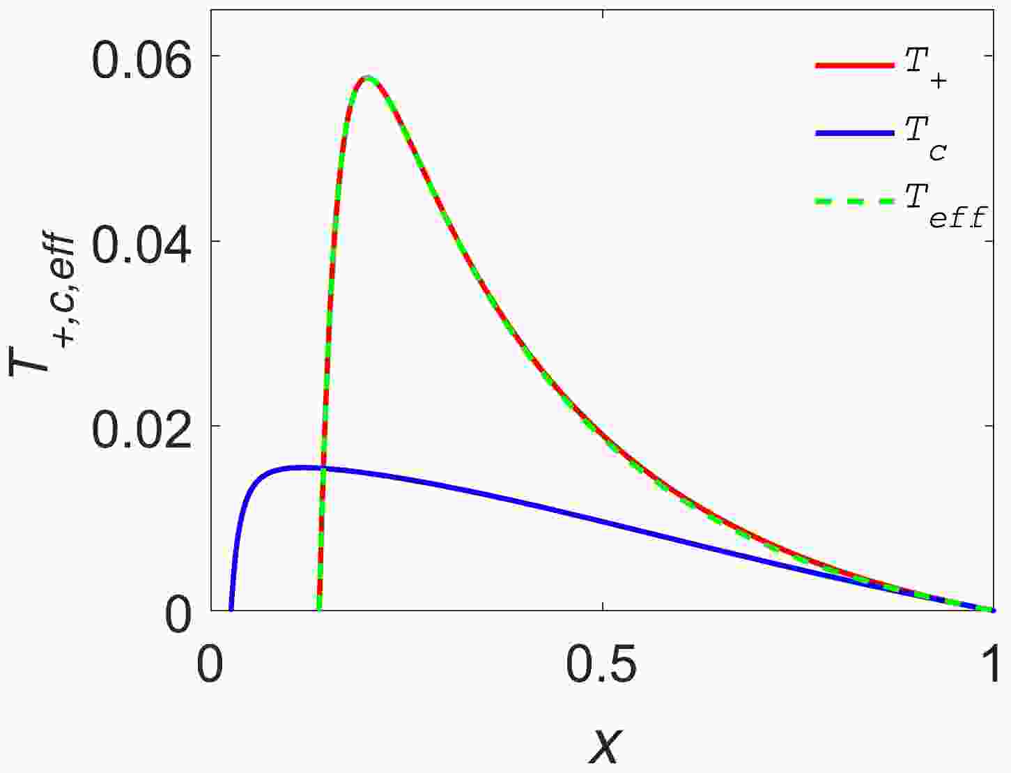
$ T_{\it{\rm{eff}}}(T_{+}, T_{c})-x $ curves are shown in Fig. 1. We find that when the hair parameter H, charge Q, and$ r_{c} $ are given, the variation in the effective temperature$ \it{T_{\rm{eff}}} $ of five-dimensional de Sitter hairy spacetime and Hawking radiation temperature$ T_{+} $ of the black hole event horizon with the ratio x of the positions of the two event horizons basically coincide. This shows that when the position$ r_{c} $ , parameter H, and charge Q are given, and when studying the thermodynamic properties of five-dimensional de Sitter hairy spacetime, the effective temperature of the spacetime can be replaced by the Hawking radiation temperature of the black hole event horizon, which simplifies the calculation.
Figure 1. (color online) Radiation temperature
$ T_{c}, T_{+} $ and effective temperature$ \it{T_{\rm{eff}}} $ vary with the ratio x of the two horizons. Other parameters are$H=1, \,Q=1, \,r_{c}=10$ .The
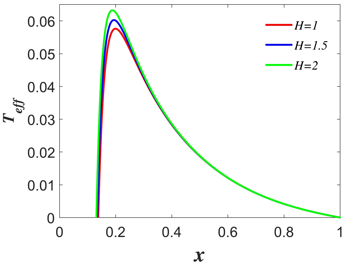
$ T_{\it{\rm{eff}}}-x $ curves of five-dimensional de Sitter hairy spacetime for different values of H are shown in Fig. 2. We find that the influence of the hair parameter H on the curve of the effective temperature varying with the position ratio x of the two horizons is only at the highest effective temperature and not at other locations. -
Now, we want to discover whether there are any hidden phase transitions that either the black hole or the full system undergo. We do not study the thermodynamic behavior of each and every parameter but focus on analyzing the Gibbs free energy, with the equilibrium state being the global minimum of this quantity. The latter can be considered in the grandcanonical ensemble, in which the charge is considered variable and the potential is fixed. Alternatively, we can consider the canonical ensemble in which charge is the fixed parameter.
There are many phases in thermodynamic systems, and each phase can exhibit significantly different macroscopic behaviors. Generally, when the temperature decreases, the system becomes more orderly. The cohesive force tries to overcome the thermal motion, and the atoms themselves are arranged into a more orderly state. Phase transition often occurs suddenly at a certain critical temperature. The study of phase transitions is one of the most interesting fields in statistical physics.
Critical points play a unique role in phase transition theory. When a system approaches its critical point from high temperature, it begins to adjust itself at the micro level and there is a large fluctuation. At this time, new order parameters will appear at the critical point. At the critical point, some thermodynamic quantities become infinite. Critical points can appear in a variety of systems, and when approaching these points, the behaviors of the systems show great similarities. Therefore, a field devoted to the study of critical phenomena has formed in physics. To extensively study the thermodynamic properties of charged de Sitter hairy spacetime and the microstructure of the system, it is necessary to discuss the phase transition behavior of charged de Sitter hairy spacetime.
The critical point denoting a second-order phase transition is determined by the following equation:
$ \begin{equation} \left(\frac{\partial \it{P_{\rm{eff}}}}{\partial V}\right)_{\it{T_{\rm{eff}}}, Q, H}=\left(\frac{\partial^{2} \it{P_{\rm{eff}}}}{\partial V^{2}}\right)_{\it{T_{\rm{eff}}}, Q, H}=0. \end{equation} $

(42) From Eq. (42), we can obtain the critical values under different parameters, as shown in Table 1.
$ x_{c} $ 

$ r_{c}^c $ 

$ \it{T_{c}^c} $ 

$ \it{P_{c}^c} $ 

H=1 Q=0.9 0.7156 3.9084 0.0164 0.002 Q=0.95 0.7184 3.916 0.0159 0.0019 Q=1 0.7216 3.9213 0.0154 0.0018 Q=1 H=1.5 0.7177 3.915 0.0161 0.0019 H=2 0.7140 3.9054 0.0168 0.002 Table 1. Critical values for different H and Q.
We can draw a phase diagram to see the phase structure near the critical point. From Eqs. (19), (32), and (34), we can construct isothermal
$ \it{P_{\rm{eff}}}-V $ curves. We exhibit the phase transition diagrams undergoing the isothermal processes in Fig. 3. We find that for$ \it{T_{\rm{eff}}} < T_{c} $ , the phase transition of five-dimensional de Sitter hairy spacetime emerges, whereas there is no phase transition for$ \it{T_{\rm{eff}}} >T_{c} $ .
Figure 3. (color online) Isothermal
$ \it{P_{\rm{eff}}}(x)-V(x) $ curves for different effective temperatures$ \it{T_{\rm{eff}}} $ . Other parameters are$ Q=H=1 $ .In Fig. 4, we give the isothermal
$P_{\rm{eff}}(x)-V(x) $ curves for different charges Q. We find that for Q = 0.9, the phase transition of five-dimensional de Sitter hairy spacetime emerges.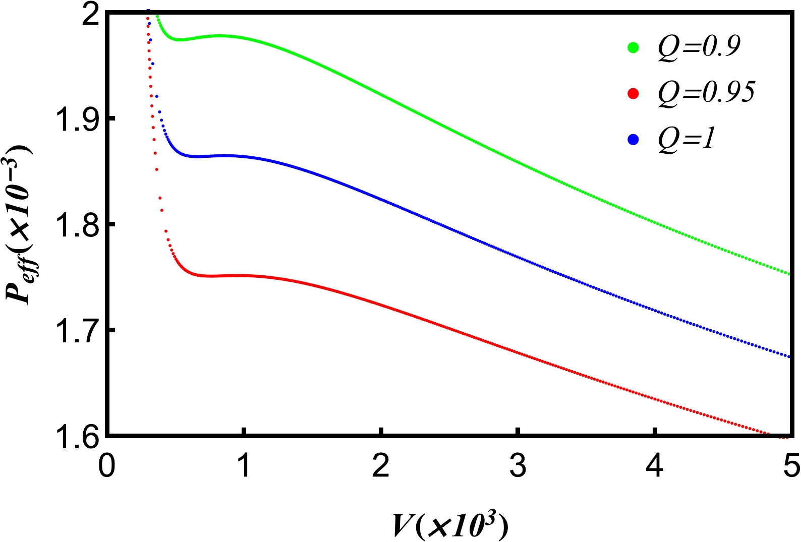
Figure 4. (color online) Isothermal
$ \it{P_{\rm{eff}}}(x)-V(x) $ curves for different charges Q. Other parameters are$H=1, \,\it{T_{c}}=\it{T_{c}^c}$ .In Fig. 5, we give the isothermal
$P_{\rm{eff}}(x)-V(x) $ curves for different hair parameters H. We find that for H = 2, the phase transition of five-dimensional de Sitter hairy spacetime emerges.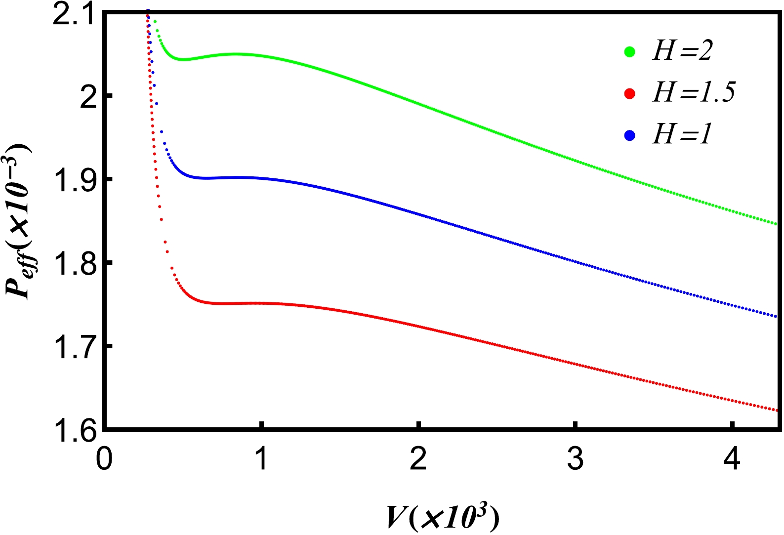
Figure 5. (color online) Isothermal
$ \it{P_{\rm{eff}}}(x)-V(x) $ curves for different hair parameters H. Other parameters are$Q=1, $ $ \it{T_{c}}=\it{T_{c}^c}$ .The Gibbs free energy is
$ \begin{equation} G(r_{c},x)=M-\it{T_{\rm{eff}}}S+\it{P_{\rm{eff}}}V, \end{equation} $

(43) where
$ \begin{aligned}[b]\\[-8pt] M=&\frac{3\pi r_{c}^2 x^2}{8(1+x^2)}-\frac{3\pi (1+x+x^2+x^3+x^4)H}{8r_{c} x(1+x)(1+x^2)}\\&+\frac{{\pi}^2 Q^2 (1+x^2+x^4)}{2x^2 r_{c}^2(1+x^{2})}, \end{aligned} $

(44) $ \begin{equation} \begin{aligned} \it{T_{\rm{eff}}}S&=\it{T_{\rm{eff}}}\frac{\pi^2 r_{c}^2}{2}F(x), \end{aligned} \end{equation} $

(45) $ \begin{equation} \it{P_{\rm{eff}}}V = \frac{\pi r_{c}^2(1-x^4)}{16}\bigg[f_{4}(x) + \frac{H f_{5}(x)}{r_{c}^3} - \frac{4\pi Q^2 f_{6}(x)}{r_{c}^4}\bigg], \end{equation} $

(46) and hence, we can obtain the expression for the Gibbs free energy,
$ \begin{aligned}[b] G(r_{c},x)=&M-\it{T_{\rm{eff}}}S+\it{P_{\rm{eff}}}V=\frac{\pi r_{c}^2}{2}\Bigg[\frac{3x^{2}}{4(1+x^{2})}\\&-\frac{3 (1+x+x^2+x^3+x^4)H}{4r_{c}^3 x(1+x)(1+x^2)}+\frac{\pi Q^2 (1+x^2+x^4)}{x^2 r_{c}^4(1+x^2)}\\&+\frac{(1-x^4)4\pi Q^2 f_{6}(x)}{8r_{c}^4} + \frac{(1-x^4)f_{c}(x)-8\it{T_{\rm{eff}}}\pi r_{c}F(x)}{8}\\&-\frac{(1-x^4)Hf_{5}(x)}{8r_{c}^3}\Bigg].\\ \end{aligned} $

(47) From Eqs. (34) and (47), we can construct isothermal
$ G-\it{P_{\rm{eff}}} $ curves. As shown in Fig. 6, for low temperatures, the swallow tail behavior appears. At the effective critical temperature, this characterized behavior disappears. Beyond the critical point, the Gibbs free energy is an increasing function of pressure, and no phase transition emerges. By reading out the self-cross point, we can obtain the first-order phase transition of the system.
Figure 6. (color online) Isothermal
$ G-\it{P_{\rm{eff}}} $ curves for different effective temperatures$ \it{T_{\rm{eff}}} $ . The effective temperature is set to 0.98$ \it{T_{\rm{eff}}^c} $ (blue line), 1.00$ \it{T_{\rm{eff}}^c} $ (red line), and 1.02$ \it{T_{\rm{eff}}^c} $ (green line). The swallow tail appears in the figure for$ \it{T_{\rm{eff}}}<\it{T_{\rm{eff}}^c} $ .As shown in Figs. 7 and 8, when the effective temperature and pressure are the same, the Gibbs free energy of spacetime increases with the increase in the charge Q and decreases with the increase in the hair parameter H.

Figure 7. (color online) Gibbs free energy G of five-dimensional de Sitter hairy spacetime as a function of effective pressure
$ \it{P_{\rm{eff}}} $ for different charges Q and fixed effective temperature$ \it{T_{\rm{eff}}}=\it{T_{\rm{eff}}^{c}} $ and hair parameter$ H=1 $ . The effective pressure$ \it{P_{\rm{eff}}} $ decreases with Q.
Figure 8. (color online) Gibbs free energy G of five dimensional de Sitter hairy spacetime as a function of effective pressure
$ \it{P_{\rm{eff}}} $ for different hair parameters H and fixed effective temperature$ \it{T_{\rm{eff}}}=\it{T_{\rm{eff}}^{c}} $ and charge$ Q=1 $ . The effective pressure$ \it{P_{\rm{eff}}} $ decreases with H.The isobaric
$ G-\it{T_{\rm{eff}}} $ curve can be constructed from Eqs. (32) and (47), as shown in Fig. 9.
Figure 9. (color online) Gibbs free energy G of five dimensional de Sitter hairy spacetime as a function of effective temperature
$ \it{T_{\rm{eff}}} $ for fixed pressure$ \it{P_{\rm{eff}}}=\it{P_{\rm{eff}}^{c}} $ . Other parameters are$ Q=H=1 $ .The entropy
$ S=-\left(\dfrac{\partial G}{\partial \it{T_{\rm{eff}}}}\right)_{\it{P_{\rm{eff}}}} $ . In the Ehrenfest classification, an entropy discontinuity with temperature is connected to discontinuous or first order phase transitions, and in the continuous or second higher order phase transitions, entropy continuously varies with temperatureThe isobaric
$ S-\it{T_{\rm{eff}}} $ curve can be constructed from Eqs. (20) and (32). Fig. 10 shows that the entropy S varies continuously with effective temperature$ \it{T_{\rm{eff}}} $ near the critical points for a fixed effective pressure$ \it{P_{\rm{eff}}} $ .
Figure 10. (color online) Entropy S varies with the effective temperature
$ \it{T_{\rm{eff}}} $ . Other parameters are$ Q=H=1, \it{P_{\rm{eff}}}=\it{P_{\rm{eff}}^{c}} $ .The heat capacity at constant pressure is
$ \begin{equation} \begin{aligned} C_{\it{P_{\rm{eff}}},Q, H} &=\it{T_{\rm{eff}}}\left(\frac{\partial S}{\partial \it{T_{\rm{eff}}}}\right)_{\it{P_{\rm{eff}}},Q,H}=\it{T_{\rm{eff}}} \frac{\dfrac{\partial S}{\partial x}\dfrac{\partial \it{P_{\rm{eff}}}}{\partial r_+}-\dfrac{\partial S}{\partial r_+}\dfrac{\partial \it{P_{\rm{eff}}}}{\partial x}}{\dfrac{\partial \it{T_{\rm{eff}}}}{\partial x}\dfrac{\partial \it{P_{\rm{eff}}}}{\partial r_+}-\dfrac{\partial \it{P_{\rm{eff}}}}{\partial r_+}\dfrac{\partial \it{T_{\rm{eff}}}}{\partial x}}. \end{aligned} \end{equation} $

(48) The isobaric
$ \it{C_{P_{\rm{eff}}}}-\it{T_{\rm{eff}}} $ curve can be constructed from Eqs. (32) and (48)The isobaric expansion coefficient is
$ \begin{equation} \begin{aligned} \alpha&=\frac{1}{V}\left(\frac{\partial V}{\partial \it{T_{\rm{eff}}}}\right)_{\it{\it{P_{\rm{eff}},Q,H}}}=\frac{1}{V} \frac{\dfrac{\partial V}{\partial x}\dfrac{\partial \it{P_{\rm{eff}}}}{\partial r_{c}}-\dfrac{\partial V}{\partial r_{c}}\dfrac{\partial \it{P_{\rm{eff}}}}{\partial x}}{\dfrac{\partial \it{T_{\rm{eff}}}}{\partial x}\dfrac{\partial \it{P_{\rm{eff}}}}{\partial r_{c}}-\dfrac{\partial \it{T_{\rm{eff}}}}{\partial r_{c}}\dfrac{\partial \it{P_{\rm{eff}}}}{\partial x}}. \end{aligned} \end{equation} $

(49) We can construct isobaric
$ \alpha-\it{T_{\rm{eff}}} $ curves from Eqs. (32) and (49), as shown in Figs. 12 and 13.
Figure 12. (color online) Isobaric expansion coefficient α as a function of the effective temperature
$ \it{T_{\rm{eff}}} $ near the critical point with different electric charges Q. Other parameters are$ H=1, \it{P_{\rm{eff}}}=\it{P_{\rm{eff}}^{c}} $ .
Figure 13. (color online) Isobaric expansion coefficient α as a function of the effective temperature
$ \it{T_{\rm{eff}}} $ near the critical point with different hair parameters H. The isobaric$ \alpha-\it{T_{\rm{eff}}} $ curves. Other parameters are$ Q=1, \it{P_{\rm{eff}}}=\it{P_{\rm{eff}}^{c}} $ .The isothermal compression coefficient is
$ \begin{equation} \begin{aligned} \kappa_{\it{T_{\rm{eff}}}}&=\frac{1}{V}\left(\frac{\partial V}{\partial \it{P_{\rm{eff}}}}\right)_{\it{\it{T_{\rm{eff}},Q,H}}}=\frac{1}{V} \frac{\dfrac{\partial V}{\partial x}\dfrac{\partial \it{T_{\rm{eff}}}}{\partial r_{c}}-\dfrac{\partial V}{\partial r_{c}}\dfrac{\partial \it{T_{\rm{eff}}}}{\partial x}}{\dfrac{\partial \it{T_{\rm{eff}}}}{\partial x}\dfrac{\partial \it{P_{\rm{eff}}}}{\partial r_{c}}-\dfrac{\partial \it{T_{\rm{eff}}}}{\partial r_{c}}\dfrac{\partial \it{P_{\rm{eff}}}}{\partial x}}. \end{aligned} \end{equation} $

(50) Isothermal
$ \kappa_{\it{T_{\rm{eff}}}}-\it{P_{\rm{eff}}} $ curves can be constructed from Eqs. (32) and (50), as shown in Figs. 14 and 15.
Figure 14. (color online) Isothermal compression coefficient as a function of the effective pressure
$ \it{P_{\rm{eff}}} $ near the critical point with different electric charges Q. The isobaric$ \kappa_{\it{T_{\rm{eff}}}}-\it{P_{\rm{eff}}} $ curves. Other parameters are$ H=1, \it{T_{\rm{eff}}}=\it{T_{\rm{eff}}^{c}} $ .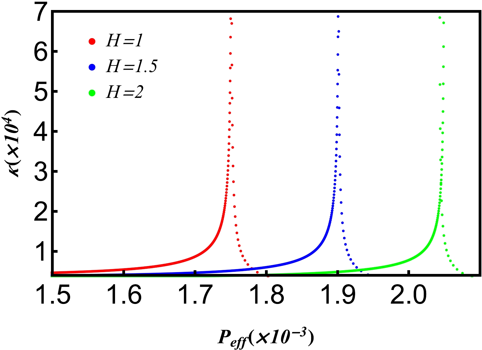
Figure 15. (color online) Isothermal compression coefficient as a function of the effective pressure
$ \it{P_{\rm{eff}}} $ near the critical point with different hair parameters H. The isobaric$ \kappa_{\it{T_{\rm{eff}}}}-\it{P_{\rm{eff}}} $ curves. Other parameters are$ Q=1, \it{T_{\rm{eff}}}=\it{T_{\rm{eff}}^{c}} $ .The heat capacity at constant volume is
$ \begin{equation} \begin{aligned} C_{V,Q}&=\it{T_{\rm{eff}}}\left(\frac{\partial S}{\partial \it{T_{\rm{eff}}}}\right)_{V,Q,H}=\it{T_{\rm{eff}}} \frac{\dfrac{\partial S}{\partial x}\dfrac{\partial V}{\partial r_{c}}-\dfrac{\partial S}{\partial r_{c}}\dfrac{\partial V}{\partial x}}{\dfrac{\partial \it{T_{\rm{eff}}}}{\partial x}\dfrac{\partial V}{\partial r_{c}}-\dfrac{\partial \it{T_{\rm{eff}}}}{\partial r_{c}}\dfrac{\partial V}{\partial x}}. \end{aligned} \end{equation} $

(51) Substituting
$ r_{c}^4 = \dfrac{2V}{\pi^2(1-x^4)} $ into Eqs. (32) and (51), we can construct isochore$ C_{V}-\it{T_{\rm{eff}}} $ curves, as shown in Figs. 16 and 17.
Figure 16. (color online) Heat capacity as a function of the effective temperature
$ \it{T_{\rm{eff}}} $ near the critical point with different electric charges Q. The isobaric$ C_{v}-\it{T_{\rm{eff}}} $ curves. Other parameters are$ H=1, V=\it{V_{\rm{eff}}^c} $ .
Figure 17. (color online) Heat capacity as a function of the effective temperature
$ \it{T_{\rm{eff}}} $ near the critical point with different hair parameters H. The isobaric$ C_{v}-\it{T_{\rm{eff}}} $ curves. Other parameters are$ Q=1, V=V_{\it{\rm{eff}}}^{c} $ .As shown in Figs. 16 and 17, the heat capacities at constant volume of five dimensional de Sitter hairy spacetime described by equivalent thermodynamics are not zero, which is different from the case of AdS black holes. However, it is a universal law for ordinary thermodynamic systems that the heat capacity of equal volume is not zero. Therefore, it is more universal to describe the thermodynamic properties of de Sitter spacetime with equivalent thermodynamic quantities.
-
When the hair parameter and charge of spacetime are given, the isothermal
$ G-\it{P_{\rm{eff}}} $ and isobaric$ G-\it{T_{\rm{eff}}} $ curves reveal that the Gibbs free energy of the two phases at the phase transition point is continuous, and the first partial derivative of the Gibbs free energy$ S=-\left(\frac{\partial G}{\partial \it{T_{\rm{eff}}}}\right)_{\it{P_{\rm{eff}}}} $ is continuous. From Figs. 10 and 11, we know that the second partial derivative of the Gibbs free energy has a sudden change. According to Ehrenfest's classification of phase transition, the phase transition at the critical point of five dimensional de Sitter hairy spacetime described by the equivalent thermodynamic quantity meets the conditions for the second order phase transition of the thermodynamic system. The second order phase transition has no latent heat of the phase transition and sudden change in volume. The thermodynamic states of the two phases at the phase transition point are the same, and there is no coexistence of the two phases. However, there are sudden changes in the constant pressure heat capacity$ C_{p_{\it{\rm{eff}}}} $ , constant pressure expansion coefficient α, and constant temperature compressibility coefficient$ \kappa_{p_{\it{\rm{eff}}}} $ . Ehrenfest derived a slope formula for the pressure at the second order phase transition point with temperature based on the condition that the entropy and volume changes of the two phases at adjacent phase transition points are equal.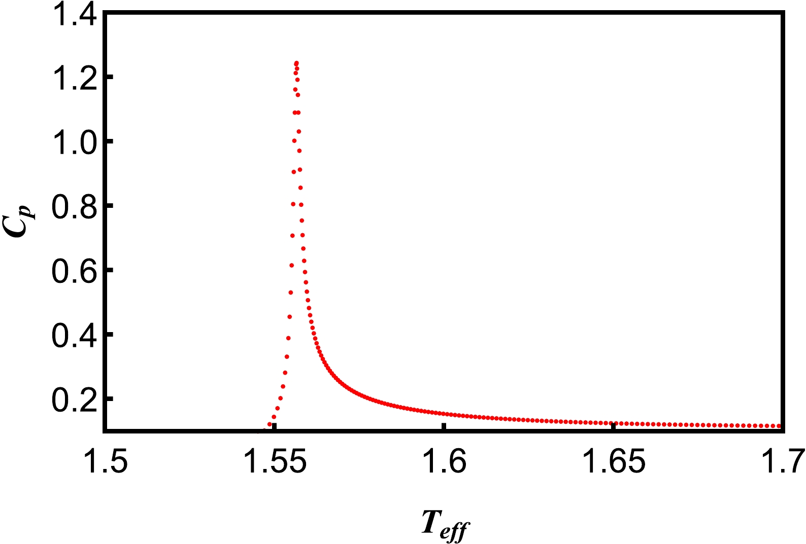
Figure 11. (color online) Heat capacity at constant pressure
$ C_{p} $ as a function of the effective temperature$ \it{T_{\rm{eff}}} $ near the critical point. Other parameters are$ Q=H=1, \it{P_{\rm{eff}}}=\it{P_{\rm{eff}}^{c}} $ .$ \begin{align} \left(\frac{\partial \it{P_{\rm{eff}}}}{\partial \it{T_{\rm{eff}}}}\right)_{S}&=\frac{C_{\it{P_{\rm{eff}}}}^2-C_{\it{P_{\rm{eff}}}}^1}{\it{T_{\rm{eff}}^c}V^c(\alpha^{2}-\alpha^{1})}=\frac{\Delta C_{\it{P_{\rm{eff}}}}}{\it{T_{\rm{eff}}^c}V^c \Delta \alpha}, \end{align} $

(52) $ \begin{align} \left(\frac{\partial \it{P_{\rm{eff}}}}{\partial \it{T_{\rm{eff}}}}\right)_{V}&=\frac{\alpha^{2}-\alpha^{1}}{\kappa_{\it{T_{\rm{eff}}}}^2-\kappa_{\it{T_{\rm{eff}}}}^1}=\frac{\Delta \alpha}{\Delta \kappa_{\it{T_{\rm{eff}}}}}, \end{align} $

(53) where the superscripts 1 and 2 represent phases 1 and 2, respectively. According to the Maxwell relations
$ \begin{equation} \left(\frac{\partial \it{P_{\rm{eff}}}}{\partial \it{T_{\rm{eff}}}}\right)_{S} = \left(\frac{\partial S}{\partial V}\right)_{\it{P_{\rm{eff}}}},\quad \left(\frac{\partial \it{P_{\rm{eff}}}}{\partial \it{T_{\rm{eff}}}}\right)_{V}=\left(\frac{\partial S}{\partial V}\right)_{\it{T_{\rm{eff}}}}, \end{equation} $

(54) where Eq. (54) is the universal relation satisfied by the system, we can get
$ \begin{equation} \left[\left(\frac{\partial \it{T_{\rm{eff}}}}{\partial \it{P_{\rm{eff}}}}\right)_{s}\right]^{c} = \left[\left(\frac{\partial V}{\partial S}\right)_{\it{P_{\rm{eff}}}} \right]^{c}, \; \left[\left(\frac{\partial \it{T_{\rm{eff}}}}{\partial \it{P_{\rm{eff}}}}\right)_{V}\right]^{c} = \left[\left(\frac{\partial V}{\partial S}\right)_{\it{T_{\rm{eff}}}}\right]^{c}, \end{equation} $

(55) where the footnote "c" denotes the values of physical quantities at the critical point. Substituting Eq. (55) into Eqs. (52) and (53),
$ \begin{equation} \frac{\Delta C_{\it{P_{\rm{eff}}}}}{\it{T_{\rm{eff}}}^{c} V^{c} \Delta \alpha} = \left[\left(\frac{\partial S}{\partial V}\right)_{\it{P_{\rm{eff}}}} \right]^{c}, \quad \frac{\Delta \alpha}{\Delta \kappa_{\it{T_{\rm{eff}}}}} = \left(\frac{\partial S}{\partial V}\right)_{\it{P_{\rm{eff}}}}^{c}. \end{equation} $

(56) According to Eq. (42), we can obtain
$ \begin{equation} \left(\frac{\partial S}{\partial V}\right)_{\it{T_{\rm{eff}}}}^{c}=\left(\frac{\partial S}{\partial V}\right)_{\it{P_{\rm{eff}}}}^{c}. \end{equation} $

(57) So far, we have proved that both the Ehrenfest equations are correct at the critical point. Utilizing Eqs. (56) and (57), the Prigogine-Defay (PD) ratio can be calculated as
$ \begin{equation} \begin{aligned} \prod =\frac{\Delta C_{\it{P_{\rm{eff}}}}\kappa_{\it{T_{\rm{eff}}}}}{\it{T_{\rm{eff}}}^{c} V^{c} (\Delta \alpha)^2}=1. \end{aligned} \end{equation} $

(58) The definition of the PD ratio was presented by Prigogine and Defay [72] and reviewed in Ref. [73]. The PD ratio can be used to measure the deviation from the second Ehrenfest equation. For the second order phase transition, the PD ratio is 1. For a PD ratio of
$ 2-5 $ , the phase transition is referred to as glassy [74]. The validity of both Ehrenfest equations shows once again that the phase transition at the critical point of criticality$ \it{P_{\rm{eff}}}-V $ in five-dimensional de Sitter hairy spacetime is a second order transition, which is consistent with the nature of the liquid-gas transition at the critical point. This conclusion is similar to that in AdS spacetime [32, 75, 76]. -
In this study, we use the basic idea that the thermodynamic quantities of de Sitter spacetime satisfy the first law of thermodynamics. When the radiation temperature of the black hole event horizon is equal to that of the cosmic event horizon, the effective temperature of the spacetime is also equal to these radiation temperatures, which can be used to obtain the five-dimensional de Sitter hairy spacetime entropy. Then, we obtain the equivalent thermodynamic quantities of spacetime. Through a discussion on the equivalent thermodynamic quantities of spacetime, we find that the thermodynamic system of five-dimensional de Sitter hairy spacetime described by the equivalent thermodynamics not only satisfies the relationship between the general thermodynamic system and the first law of thermodynamics satisfied by the AdS black hole, but also obeys the Smarr formula of the black hole.
It is known from the discussion in Sec. III that the second order phase transition in five-dimensional de Sitter Hair spacetime described by equivalent thermodynamics is similar to that in van der Waals systems and AdS black holes. When the hair parameter H is given, the critical effective temperature and pressure decrease with the increase in the charge Q, and when the charge Q is given, the critical effective temperature and pressure increase with the increase in the hair parameter H.
In Sec. IV, we perform an analytical check of Ehrenfest equations and derive the specific heat, expansion coefficient, and the equal compressibility of five-dimensional de Sitter hairy spacetime. We find that the five-dimensional de Sitter hairy spacetime system undergoes a second order equilibrium phase transition at the critical point. This result is similar to the nature of the van der Waals liquid-gas phase transition at the critical point.
Through the discussion on the thermodynamic properties of five-dimensional de Sitter hairy spacetime described by equivalent thermodynamic quantities, we find that the equivalent heat capacity of spacetime is not zero, which is different from the case of AdS but consistent with that of general thermodynamic systems. This shows that it is of greater general physical significance for us to describe the thermodynamic properties of dS spacetime using equivalent thermodynamic quantities. It lays a foundation for us to further discuss the thermodynamic properties of dS spacetime. Because our universe is an asymptotic dS spacetime, the discussion on the thermodynamic properties of five-dimensional de Sitter hairy spacetime will help us understand the evolution of spacetime and seek a theoretical basis for our exploration of the physical mechanism behind the accelerated expansion of the universe.
-
We would like to thank Prof. Zong-Hong Zhu and Meng-Sen Ma for indispensable discussions and comments.
-
Data Availability Statement: No Data associated with the manuscript.
Thermodynamic quantities and phase transitions of five-dimensional de Sitter hairy spacetime
- Received Date: 2023-06-06
- Available Online: 2023-10-15
Abstract: In this study, we take the mass, electric charge, hair parameter, and cosmological constant of five-dimensional de Sitter hairy spacetime as the state parameters of the thermodynamic system, and when these state parameters satisfy the first law of thermodynamics, the equivalent thermodynamic quantities of spacetime and the Smarr relation of five-dimensional de Sitter hairy spacetime are obtained. Then, we study the thermodynamic characteristics of the spacetime described by these equivalent thermodynamic quantities and find that de Sitter hairy spacetime has a phase transition and critical phenomena similar to those of van de Waals systems or charged AdS black holes. It is shown that the phase transition point of de Sitter hairy spacetime is determined by the ratio of two event horizon positions and the cosmic event horizon position. We discuss the influence of the hair parameter and electric charge on the critical point. We also find that the isochoric heat capacity of the spacetime is not zero, which is consistent with the ordinary thermodynamic system but differs from the isochoric heat capacity of AdS black holes, which is zero. Using the Ehrenfest equations, we prove that the critical phase transition is a second order equilibrium phase transition. Research on the thermodynamic properties of five-dimensional de Sitter hairy spacetime lays a foundation for finding a universal de Sitter spacetime thermodynamic system and studying its thermodynamic properties. Our universe is an asymptotically dS spacetime, and the thermodynamic characteristics of de Sitter hairy spacetime will help us understand the evolution of spacetime and provide a theoretical basis to explore the physical mechanism of the accelerated expansion of the universe.


 Abstract
 HTML
HTML Reference
 Related
 PDF
PDF




 DownLoad: