


 Abstract
 HTML
HTML Reference
 Related
 PDF
PDF


-
Recent investigations have shown that a strong magnetic field may exist in at least two high-energy astrophysical objects. First, the magnetic fields on the surface of magnetars are expected to reach
$ 10^{15} $ G, whereas in the inner core of magnetars, the magnitude of the magnetic fields could be of the order of$ 10^{18} $ G [1]. Second, it is considered that during the electroweak phase transition in the early universe, extremely strong magnetic fields exceeding$ 10^{20} $ G might have been produced [2]. In the course of relativistic non-central heavy-ion collisions, the strength of magnetic fields can reach up to$ 10^{18} $ G at the Relativistic Heavy Ion Collider (RHIC) and$ 10^{20} $ G at the Large Hadron Collider (LHC) [3, 4]. Although such strong magnetic fields in these heavy-ion colliding experiments decay during a very short period, they can still induce significant effects on the phase structure of QCD matter. Many theoretical investigations based on the lattice QCD method or effective QCD theories, such as NJL models, have shown that strong magnetic fields can modify the quark potential and meson properties owing to complex QED-QCD interactions [5–7]. However, there are relatively few studies in regard to the modification of baryon properties in the presence of strong magnetic fields [8–10].It is difficult to study low-energy strong interaction physics directly from QCD theory owing to its non-perturbative character at the low-energy scale. Alternative approaches, such as lattice QCD or effective field theories (EFTs), must instead be considered. The Skyrme model, a promising EFT, was first proposed by Skyrme in 1961 [11]. In this model, meson fields are the basic degrees of freedom, and baryons emerge as collective excitations or topological solitons, known as skyrmions, from nonlinear interactions between mesons, the topological charge of which is identified by the baryon number. The Lagrangian of the standard Skyrme model consists of three terms. The first is the sigma-model term, quadratic in its first derivatives, which provides the kinetic energy of π mesons, the second is the Skyrme term, which is quartic in its first derivatives, and relates to the stable solutions of models, and the third is the potential term, which gives explicit breaking of chiral symmetry and relates to the π meson mass. Although this standard Skyrme model can successfully describe many nuclear phenomena, there are still several defects. For example, it provides excessively high binding energies of atomic nuclei and thus is generally difficult to apply to the investigation of matter with a large baryon number. Many efforts have been made to improve the standard Skyrme model (see, for example, Refs. [12–18] and the references therein). In recent years, so-called generalized Skyrme models have been proposed [19, 20], where a term sextic in derivatives is added and may be related to vector meson exchange based on phenomenological arguments, which can overcome the shortcomings of the original Skyrme models.
In this study, we modify the method proposed by Ref. [8] to study the deuteron as a
$ B=2 $ skyrmion. Besides the conventional Skyrme model (labeled as the SKM), the effects of the derivative dependent sextic Lagrangian term are also considered (labeled as the gSKM). This article is organized as follows: In Sec. II, we describe the formulas necessary. Here, we quantize the skyrmion within the semi-classical quantization method [21, 22]. Note that the quantization method in Ref. [8] consists of allowing the${S U}(2)$ valued field in the Skyrme model to rotate in three-dimensional isospin space and spatial space only in the x – y plane, which is inconsistent with the constraint of Eq. (21) resulting from the cylindrical symmetry implicitly imposed on the solution of the skyrmion in this study when we quantize the$ B=2 $ skyrmion. Therefore, in the present study, we modify the quantization method in Ref. [8] and consider three-dimensional rotation in spatial space as well as in isospin space. In Sec. III, the calculated results and discussions are given. Finally, a summary is presented in Sec. IV. -
In this study, the action of the Skyrme model coupled with magnetic fields is
$\Gamma_{\rm WZW}(U)+\int {\rm d}^4x \it\text{£}_0$ . Here, the Wess-Zumino-Witten (WZW) term represents chiral anomaly effects [23, 24], and the gauged WZW action$\Gamma_{\rm WZW}(U)=\Gamma_c(U)-\Gamma_c(1)$ in the presence of electromagnetic fields is given in Ref. [25], with$ \begin{aligned}[b] \Gamma_{c}(U)=&-\frac{\rm i}{80\pi^2}\int {\rm d}^5x\varepsilon^{ijklm}{\mathrm{Tr}}[R_iR_jR_kR_lR_m]\\ &+\frac{1}{16\pi^2}\int {\rm d}^4x\varepsilon^{\mu\nu\alpha\beta}{\mathrm{Tr}}\Big\{eA_{\mu}Q_E(R_{\nu}R_{\alpha}R_{\beta}\\ &+L_{\nu}L_{\alpha}L_{\beta})+\frac{{\rm i}e^2}{2}[A_{\mu}Q_ER_{\nu}A_{\alpha}Q_ER_{\beta}\\ &-A_{\mu}Q_EL_{\nu}A_{\alpha}Q_EL_{\beta}]-{\rm i}e^2[A_{\mu}Q_EU^{\dagger}\\ &A_{\nu}Q_EUR_{\alpha}R_{\beta}-A_{\mu}Q_EUA_{\nu}Q_EU^{\dagger}L_{\alpha}L_{\beta}\\ &-\partial_{\mu}A_{\nu}Q_EU^{\dagger}A_{\alpha}Q_EUR_{\beta}\\ &-\partial_{\mu}A_{\nu}Q_EUA_{\alpha}Q_EU^{\dagger}L_{\beta}-(A_{\mu}Q_E\partial_{\nu}A_{\alpha}Q_E\\ &+\partial_{\mu}A_{\nu}Q_EA_{\alpha}Q_E)(R_{\beta}+L_{\beta})]\\ &+e^3A_{\mu}Q_EA_{\nu}Q_EA_{\alpha}Q_E(R_{\beta}+L_{\beta})\\ &+e^3(A_{\mu}Q_EU^{\dagger}A_{\nu}Q_EUA_{\alpha}Q_ER_{\beta}\\ &+A_{\mu}Q_EUA_{\nu}Q_EU^{\dagger}A_{\alpha}Q_EL_{\beta}\\ &+A_{\mu}Q_EU^{\dagger}A_{\nu}Q_E\partial_{\alpha}A_{\beta}Q_EU\\ &+A_{\mu}Q_EU^{\dagger}\partial_{\nu}A_{\alpha}Q_EA_{\beta}Q_EU\\ &+\partial_{\mu}A_{\nu}Q_EA_{\alpha}Q_EU^{\dagger}A_{\beta}Q_EU\\ &+A_{\mu}Q_E\partial_{\nu}A_{\alpha}Q_EU^{\dagger}A_{\beta}Q_EU)\\ &-{\rm i} e^4(A_{\mu}Q_EA_{\nu}Q_EA_{\alpha}Q_EU^{\dagger}A_{\beta}Q_EU\\ &+A_{\mu}Q_EU^{\dagger}A_{\nu}Q_EA_{\alpha}Q_EA_{\beta}Q_EU\\ &+\frac{1}{2}A_{\mu}Q_EU^{\dagger}A_{\nu}Q_EUA_{\alpha}Q_EU^{\dagger}A_{\beta}Q_EU)\Big\}\,\,,\\ \end{aligned} $

(1) where the first term is a five-dimensional integral whose boundary is four-dimensional space-time,
$ R_i=U^{\dagger}\partial_iU $ ,$ L_i=\partial_iUU^{\dagger} $ , e is the unit electric charge, and$ Q_E= I/6+\tau_3/2 $ is the electric charge matrix, where I is the rank 2 unit matrix, and$ \tau_3 $ is the third Pauli matrix. The generalized Skyrme Lagrangian$ \text{£}_0 $ with local gauge invariance reads as$ \begin{aligned}[b] \text{£}_0=&\frac{F_{\pi}^2}{16}{\rm{Tr}}(D_{\mu}U^{\dagger} D^{\mu}U)+\frac{m_{\pi}^2F_{\pi}^2}{8}{\rm{Tr}}(U-1)\\ &+\frac{1}{32g^2}{\rm{Tr}}([U^{\dagger} D_{\mu}U,U^{\dagger} D_{\nu}U]^2)-\frac{9\pi^2}{5m^2}B^{\mu}B_{\mu}\,\,,\\ \end{aligned} $

(2) with the covariant derivative
$ D_{\mu}U $ defined as$ D_{\mu}U=\partial_{\mu}U-{\rm i}eA_{\mu}[Q_E,U]\,\,. $

(3) Here, the Lagrangian has three free parameters (
$ F_{\pi} $ , g, m), which are used to fit several experimental values. The pion mass is set to its physical value$ m_{\pi} = 138 $ MeV. In this study, the homogeneous magnetic field B along the z direction is considered, and the symmetric gauge of the electromagnetic field$ A_{\mu} $ is chosen as$A_{\mu}=(0, -yB/2,$ $ xB/2,~ 0)$ . As an${S U}(2)$ valued field, U is expressed as$ U=\exp({\rm i}F(r)\vec{\tau}\cdot\vec{n}(\theta,\varphi))\,\,, $

(4) where
$ F(r) $ is a real profile function satisfying the boundary conditions$ F(0)=\pi $ and$ F(\infty)=0 $ ,$ |\vec{n}|=1 $ . For baryon number$ B>1 $ , we utilize the so-called rational map ansatz [26], and$ \vec{n} $ is expressed as$ (n_1, n_2, n_3)=\frac{1}{1+|R|^2}(2 {\rm Re}(R), 2 {\rm Im}(R), 1-|R|^2)\,\,, $

(5) where
$ R(z) $ is the rational map between two Riemann spheres, with z as the Riemann sphere coordinate defined as$z=\tan(\theta/2)\exp({\rm i}\varphi)$ . The form of R is$ p/q $ , where p and q are polynomials in z with the larger of their degrees being B. For the$ B=2 $ skyrmion,$ R=z^2 $ is chosen. The last term in Eq. (2) is sextic in derivatives, in which$ B^{\mu} $ reads as$ B^{\mu}=\frac{1}{24\pi^2}\varepsilon^{\mu\nu\alpha\beta}{\mathrm{Tr}}[(U^{\dagger}D_{\nu}U)(U^{\dagger}D_{\alpha}U)(U^{\dagger}D_{\beta}U)]\,\,, $

(6) which degenerates into the topological current in the absence of magnetic fields.
Considering the axial symmetry imposed by magnetic fields, we follow the ansatz in Ref. [8] to deform the spatial space as
$ \begin{aligned}[b] x=&c_{\rho}r\sin(\theta)\cos(\varphi)\,, \quad y=c_{\rho}r\sin(\theta)\sin(\varphi)\, , \\ z=&c_zr\cos(\theta)\,\,, \end{aligned} $

(7) where
$ c_{\rho} $ and$ c_z $ are positive dimensionless parameters, and$ \theta\in[0,\pi] $ and$ \varphi\in[0,2\pi] $ are polar angles. Then, the volume element is${\rm d}V={\rm d}x{\rm d}y{\rm d}z=c_{\rho}^2c_zr^2\sin(\theta){\rm d}r {\rm d}\theta {\rm d}\varphi$ . The parameters$ c_{\rho} $ and$ c_z $ have two effects: they deform the shape and scale the volume. Because the scale effect of$ c_{\rho} $ and$ c_z $ can be absorbed by performing the scale transform of r, we follow the choice in Ref. [8] in which$ c_{\rho}\equiv 1/\sqrt{c_z} $ to seek results with a conserved volume. It should be mentioned that in Ref. [8], which studies$ B=1 $ baryons,$ c_z $ characterizes the deviation degree from a sphere. However, in the present study, the deuteron is toroidal and based on the rational map ansatz, which has already deviated from a sphere. Thus,$ c_z $ in this study can be understood as a new parameter introduced into the conventional rational map approximation (cRMA), and$ c_z\neq 1 $ means a deviation from the cRMA.In the semi-classical quantization method, to obtain the spin and isospin of baryons, U is given time dependence by rotating U in both space and isospin as
$ \begin{array}{*{20}{l}} \hat{U}=A(U(\tilde{S}))A^{\dagger}\,\,, \end{array} $

(8) in which A and
$ \tilde{S} $ are the rotation matrices for the isospin and spatial rotations, respectively, satisfying$ \begin{aligned}[b] A^{-1}\dot{A}=&\frac{\rm i}{2}\omega_a\tau_a\,\,,\\ (\tilde{S}^{-1}\dot{\tilde{S}})_{ij}=&-\varepsilon_{ijk}\Omega_k\,\,, \end{aligned} $

(9) where
$ a,i,j,k=1, 2, 3 $ . By replacing U with$ \hat{U} $ in$\text{£}_0$ , the static contribution to the deuteron mass can be expressed as$ \begin{array}{*{20}{l}} M_{d,st}=\langle\psi_d\mid M_0+M_1(eB)+M_2(eB)^2\mid\psi_d\rangle\,\,, \end{array} $

(10) in which
$ \begin{aligned}[b] M_0=&\left(\frac{\pi}{\beta g^2}\right)\int\frac{{\rm d}r}{12 c_z^2r^2}\Big\{3 c_z \left[16 + c_z^3 (-8 + 3 \pi)\right]\\ & + 48\left[4 + c_z^3 (-2 + \pi) - \pi\right] r^2 + 96 c_z^2 m_{\pi}^2 r^4\\ &- 96 c_z^2 m_{\pi}^2 r^4 \cos(F) - 4 \left\{c_z \left[16 + c_z^3 (-8 + 3 \pi)\right]\right.\\ &\left.+ 12 \left[4 + c_z^3 (-2 + \pi) - \pi\right] r^2\right\} \cos(2F)\\ & + c_z \left[16 + c_z^3 (-8 + 3 \pi)\right] \cos(4F)\\ &+ 4 r^2\left\{-6 c_z \left[2 + c_z^3 (-4 + \pi) - \pi\right] + 4(1 + 2 c_z^3)r^2\right.\\ &\left.+ 6 c_z \left[2 + c_z^3 (-4 + \pi) - \pi\right] \cos(2F)\right\} F'^2\\ &+4(8+3\pi)\kappa c_z^2\sin^4(F)F'^2\Big\}\,\,, \end{aligned} $

(11) $ \begin{aligned}[b] M_1=&\left(\frac{R_3S_3\pi}{\beta g^2}\right)\int\frac{ 2{\rm d}r}{3 c_z^2}\Big\{\sin^2(F)\left\{-6 c_z^2 (-4 + \pi)r^2\right.\\ &- 2 c_z^3 (28 - 9 \pi) \sin^2(F) - 2 (-32 + 9 \pi) \sin^2(F)\\ &\left.- [28 - 9 \pi + 4 c_z^3 (-10 + 3 \pi)] r^2 F'^2\right\}\\ &+4\kappa c_z\sin^4(F)F'^2\Big\}\,\,, \end{aligned} $

(12) and
$ \begin{aligned}[b] M_2=&\left(\frac{\pi}{\beta g^2}\right)\int\frac{r^2 {\rm d}r}{480 c_z^3}\Bigg\{\sin^2(F)\Big\{-40 c_z^2 \big\{2 (1 + S_3^2)\\ &[8 - 3 \pi + (-28 + 9 \pi) R_3^2]+ c_z^3 (-1 + S_3^2)\\ & [32 - 9 \pi + (-88 + 27 \pi) R_3^2]\big\} r^2+ 20 \sin^2(F)\\ &\big\{8 S_3^2 (-28 + 9 \pi + 124 R_3^2 - 39 \pi R_3^2)\\ &+ 4 c_z^6 (-1 + S_3^2) [28 - 9 \pi + 2 (-47 + 15 \pi) R_3^2] \\ &+ c_z^3 \big[128 - 39 \pi + (-448 + 141 \pi) R_3^2\\ &+ S_3^2 [80 - 27 \pi + (-400 + 129 \pi) R_3^2]\big]\big\}\\ & - 4 \big\{-8 S_3^2 [48 - 142 R_3^2 + 15 \pi (-1 + 3 R_3^2)]\\ &+ 4 c_z^6 (-1 + S_3^2) [48 - 142 R_3^2 + 15 \pi (-1 + 3 R_3^2)]\\ & + c_z^3 \big[112 - 45 \pi + 3 (-136 + 45 \pi) R_3^2 \\ & + S_3^2 [432 - 1288 R_3^2 + 135 \pi (-1 + 3 R_3^2)]\big]\big\} r^2 F'^2\Big\}\\ &+10 \kappa c_z\sin^4(F)F'^2\big\{2 S_3^2 [-8 + 3 \pi + 3 (24 - 7 \pi) \\ & R_3^2] + c_z^3 (1 - S_3^2) [16 - 3 \pi + 3 (-24 + 7 \pi) R_3^2]\big\}\Bigg\}\,\,.\\ \end{aligned} $

(13) Here,
$ \beta=2\sqrt{2}/(gF_{\pi}) $ is used as the unit of length,$ \kappa=9g^2/(5m^2\beta^2\pi^2) $ ,$ R_3 $ is defined as$ R_3= \rm{Tr}(\tau_3A^{\dagger}\tau_3A)/2 $ , and$ S_3 $ is the$ \tilde{S}_{33} $ component of the rotation matrix$ \tilde{S} $ .The replacement of U with
$ \hat{U} $ can also give the kinematical part in the form$ \begin{aligned}[b] T=&\frac{1}{2}a_i\omega_i^2+\frac{1}{2}b_i\Omega_i^2-c_i\omega_i\Omega_i+D(eB)S_3(\omega_3-2\Omega_3)\\ &+E(eB)(S_1\Omega_1+S_2\Omega_2)\,\,, \end{aligned} $

(14) where
$ i=1,2,3 $ ,$ S_1 $ and$ S_2 $ are the$ \tilde{S}_{13} $ and$ \tilde{S}_{23} $ components of the rotation matrix$ \tilde{S} $ , respectively,$ D=\int {\rm d}r\frac{r^2}{2 c_z \pi}(-4 + \pi)\sin^2( F)F'\,\,, $

(15) $ E=\int {\rm d}r\frac{r^2}{2 c_z \pi}[4-\pi+ 2c_z^3(-3 + \pi)]\sin^2( F)F'\,\,, $

(16) and
$ a_1=a_2 $ ,$ b_1=b_2 $ ,$ c_1=c_2=0 $ , and$ a_3=b_3/4=c_3/2 $ , where$ a_1=\left(\frac{2\pi\beta}{g^2}\right)\left[a_{10}+ a_{11}(eB)+a_{12}(eB)^2\right]\,\,, $

(17) $ a_3=\left(\frac{2\pi\beta}{g^2}\right)\left[a_{30}+a_{32}(eB)^2\right]\,\,, $

(18) $ b_1=\left(\frac{2\pi\beta}{g^2}\right)\left[b_{10}+ b_{11}(eB)+b_{12}(eB)^2\right]\,\,. $

(19) The equations needed in Eqs. (17)–(19) are listed in Appendix A. We can then obtain the body-fixed canonical conjugate momenta of the isospin and spin by taking functional derivatives with respect to
$ \omega_a $ and$ \Omega_a $ , respectively, as$ K_a=\frac{\partial T}{\partial\omega_a}\,\,,\quad\quad L_a=\frac{\partial T}{\partial\Omega_a}\,\,. $

(20) Note that in Ref. [8], only the spatial rotation in the x – y plane is considered, that is, only the third component of the spatial angular momentum is defined and
$ k\equiv 3 $ in Eq. (9), which results in the equivalence between the third component of the body-fixed ($\boldsymbol{L}$ ) and space-fixed ($\boldsymbol{J}$ , physically more meaningful) spatial angular momenta, that is,$ J_3=L_3 $ . When the constraint [The distinction between the baryon number B here and the magnetic field$ eB $ should always be clear by context.]$ \begin{array}{*{20}{l}} (BK_3+L_3)|\psi\rangle=0\,\,, \end{array} $

(21) which results from the cylindrical symmetry implicitly imposed on the solution of the skyrmion in this study, is cast into the calculation for the
$ B=1 $ nucleon, as in Ref. [8], there is no trouble. This is because the quantum numbers ($ j_3 $ and$ k_3 $ ) of$ J_3 $ and$ K_3 $ can simultaneously be half-integers for the$ B=1 $ nucleon. However, the integer$ j_3=1 $ for the$ B=2 $ deuteron allows$ k_3 $ to be a half-integer, according to Eq. (21), which is prohibited in the quantization of the$ B=2 $ deuteron. Therefore, in this study, we modify the quantization method in Ref. [8] and consider three-dimensional rotation in the spatial space as well as in the isospin space. As a result,$ J_3 $ and$ L_3 $ become mutually independent. Consequently, the quantum numbers ($ l_3 $ and$ k_3 $ ) of$ L_3 $ and$ K_3 $ are allowed to be zero for the$ B=2 $ deuteron, and the constraint of Eq. (21) is not violated. Here, the wave function of the deuteron is given by the direct product$ |ii_3k_3\rangle|jj_3l_3\rangle $ , where i and$ i_3 $ are the quantum numbers of the space-fixed isospin momentum ($\boldsymbol{I}^2$ and$ I_3 $ , physically more meaningful).Now, using the relations
$ J_3=-\sum S_iL_i $ and$ \sum S_i^2\equiv 1 $ , where$ i=1, 2, 3 $ , we can write the kinematical contribution to the deuteron mass as$ \begin{aligned}[b] M_{d,\rm kin}=&\langle\psi_d\mid\sum\limits_{a=1,2,3}(\omega_aK_a+\Omega_aL_a)-T\mid\psi_d\rangle\,\,,\\ =&\langle\psi_d\mid\frac{\boldsymbol{I}^2}{2a_1}+\frac{\boldsymbol{J}^2+(1-S_3^2)E^2(eB)^2}{2b_1}\\ &+\left[\frac{(K_3-S_3D(eB))^2}{2a_3}-\left(\frac{1}{a_1}+\frac{4}{b_1}\right)\frac{K_3^2}{2}\right]\\ &+\frac{(J_3-2S_3K_3)E(eB)}{b_1}\mid\psi_d\rangle\,\,. \end{aligned} $

(22) The deuteron mass is the sum of the static and kinematical contributions, that is,
$M_d=M_{d,st}+M_{d,\rm kin}$ .$ M_{d,st} $ and$M_{d,\rm kin}$ can be obtained with the help of the wave function, as stated in Ref. [20].$ F(r) $ in Eq. (4) can be obtained at the O($ N_C $ ) order by minimizing$ M_{d,st} $ , with the help of a certain value of$ c_z $ obtained by minimizing$ M_d $ .The magnetic moment of the deuteron is defined by
$ \mu\equiv-\partial M_d/\partial(eB) $ . Because$ k_3 $ is equal to zero in the wave function of the deuteron, and the expectation value of$ R_3 $ is zero [20], most of the linear terms of magnetic fields in Eqs. (10) and (22) offer no contribution to the mass, except the last term in Eq. (22). Thus the magnetic moment is given by$ \mu=-\beta^2j_3E/b_1 $ for$ |eB|=0 $ (the presence of$ \beta^2 $ results from the consideration of the unit of length in this study). This equation for the magnetic moment is equivalent to that deduced in Ref. [27]. We take the model parameters as$ g= $ 4.84 and$ F_{\pi}= $ 108 MeV for the SKM, and$ g= $ 19.48 and$ F_{\pi}= $ 129.11 MeV for the gSKM with an additional parameter m chosen as$ m= $ 420 MeV [19]. It is known that the wave function of the deuteron, as the ground state$ ^3S_1 $ of the$ B=2 $ skyrmion, is$ |000\rangle|110\rangle $ . We then obtain the results of the magnetic moment for$ |eB|=0 $ , which in the unit of the Bohr magneton$ \mu_B=1/(2M_N) $ for the SKM and gSKM are 0.69 and 0.77, which are 19% and 10% smaller, respectively, than the experimental value of 0.857. -
In Fig. 1, we illustrate the
$ |eB| $ dependence of$ c_z $ for the deuteron. We also give the calculations for the first excited state$ ^1S_0 $ , the wave function of which is$ |100\rangle|000\rangle $ , for comparison. In the absence of magnetic fields, the results slightly deviate along the direction of the magnetic field from those in cRMA, with$ c_z=1.03 $ in the SKM and$ c_z=1.05 $ in the gSKM for the deuteron, which are smaller than those for the first excited state. When the magnetic fields increase,$ c_z $ decreases continuously. The gSKM exhibits a larger descent velocity of$ c_z $ with$ |eB| $ than SKM. Overall, we see that the deviation of the calculated results from$ c_z=1 $ in the presence of the magnetic fields is$ \lesssim 10\ $ %.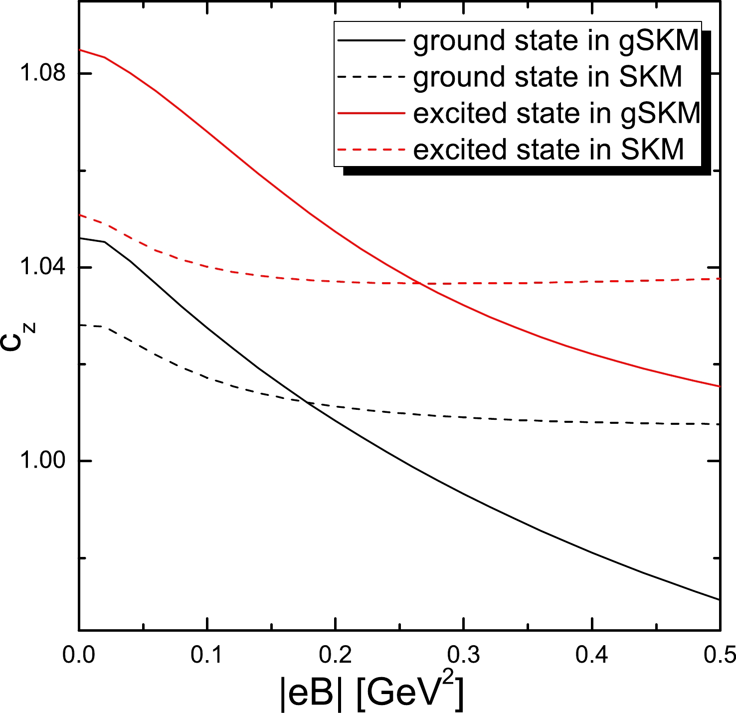
Figure 1. (color online)
$|eB|$ dependence of$c_z$ for the deuteron in the ground (color black) and excited states (color red) for the gSKM (solid curves) and SKM (dashed curves).In the deuteron under the magnetic fields, the radial density of baryon charge is given by
$ \begin{aligned}[b] \rho(r)=&\rho_0(r)+\rho_B(r)\,\,,\\ =&\frac{-4\sin^2(F)F'}{\pi}+\langle\psi_d\mid\frac{ r(eB)}{24\pi c_z}(4-\pi)R_3S_3\\ &\times[\sin(2F)+r\cos(2F)F']\mid\psi_d\rangle\,\,, \end{aligned} $

(23) where the integral of the first term
$ \rho_0(r) $ over r is 2, which is consistent with the baryon charge$ B=2 $ of the deuteron, and the second term$ \rho_B(r) $ is induced by magnetic fields. For$ B=1 $ , the presence of$ \rho_B(r) $ under magnetic fields does not break baryon number conservation because integrating it over the entire space is equal to zero [8]. The fact that$ k_3=0 $ and the expectation value of$ R_3 $ in Eq. (23) is zero [20] indicates that$ \rho_B\equiv 0 $ in the deuteron. Because$ i_3=0 $ for the deuteron, we can evaluate the root mean square (RMS) electric charge radii, defined as$ R=(\int X^2\rho_0/2dV)^{1/2} $ , in which$ X=\sqrt{x^2+y^2+z^2} $ , and$ R_x=(\int x^2\rho_0/2dV)^{1/2} $ and$ R_z=(\int z^2\rho_0/2dV)^{1/2} $ for directions of x and z, respectively. The results are illustrated in Fig. 2. The phenomenon that$ R_x $ is clearly larger than$ R_z $ is shown, which is consistent with the toroidal structure of the B=2 skyrmion. The RMS charge radii for the gSKM are larger than those for the SKM, and the calculated results for the ground state are similar to those for the excited state. Furthermore, Fig. 2 shows that R,$ R_x $ , and$ R_z $ decrease with increasing magnetic field strength, which indicates a gathering of the electric charges when the magnetic fields increase.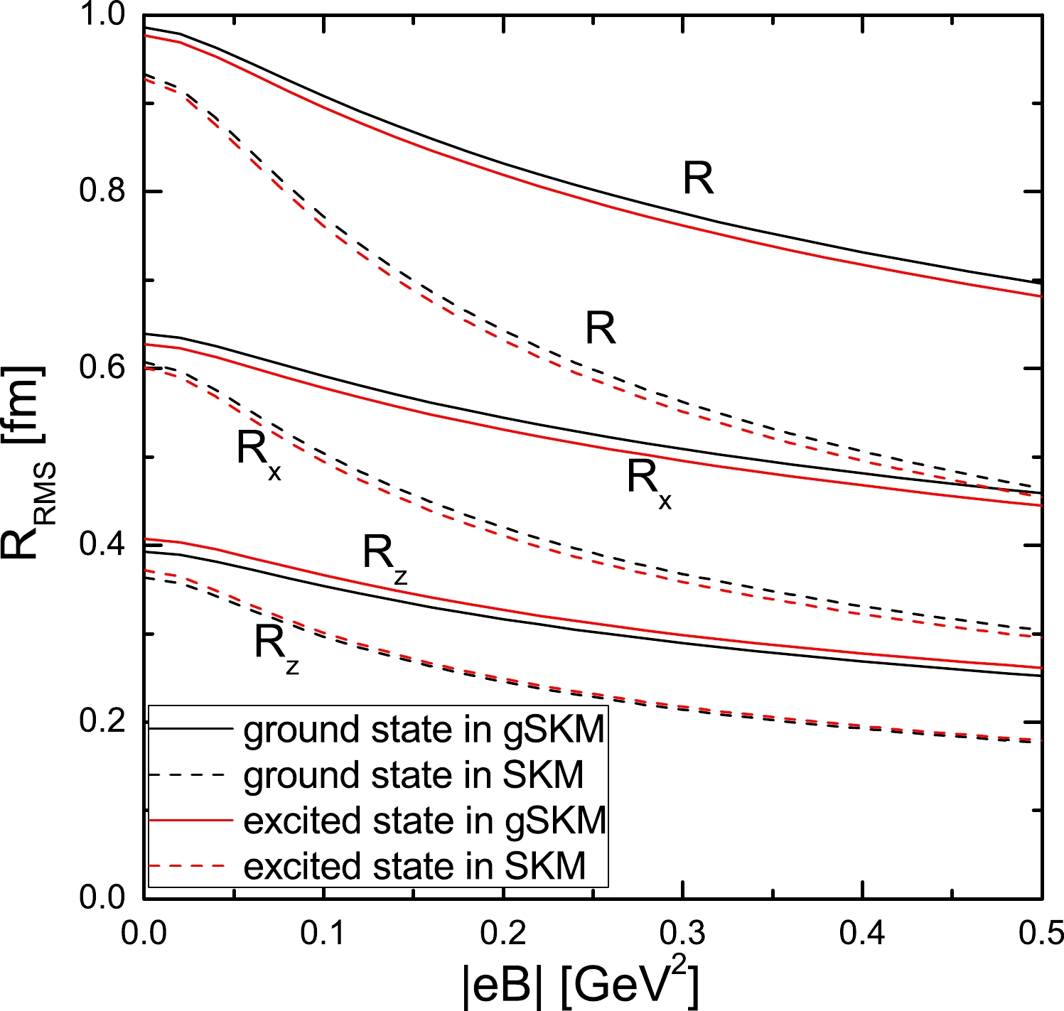
Figure 2. (color online)
$|eB|$ dependence of the RMS electric charge radii (labeled as R) of the deuteron,$R_x$ and$R_z$ for the x and z directions, in the ground (color black) and excited states (color red) for the gSKM (solid curves) and SKM (dashed curves).The results on the RMS electric charge radii in Fig. 2 can also be understood from the profile functions
$ F(r) $ , which are shown in Fig. 3. Figure 3 shows that the profile functions under magnetic fields for the gSKM are wider than those for the SKM, which is consistent with the larger RMS radii for the gSKM in Fig. 2. Moreover, the phenomenon that the increase in$ |eB| $ narrows$ F(r) $ also indicates a gathering of the electric charges when the magnetic fields increase.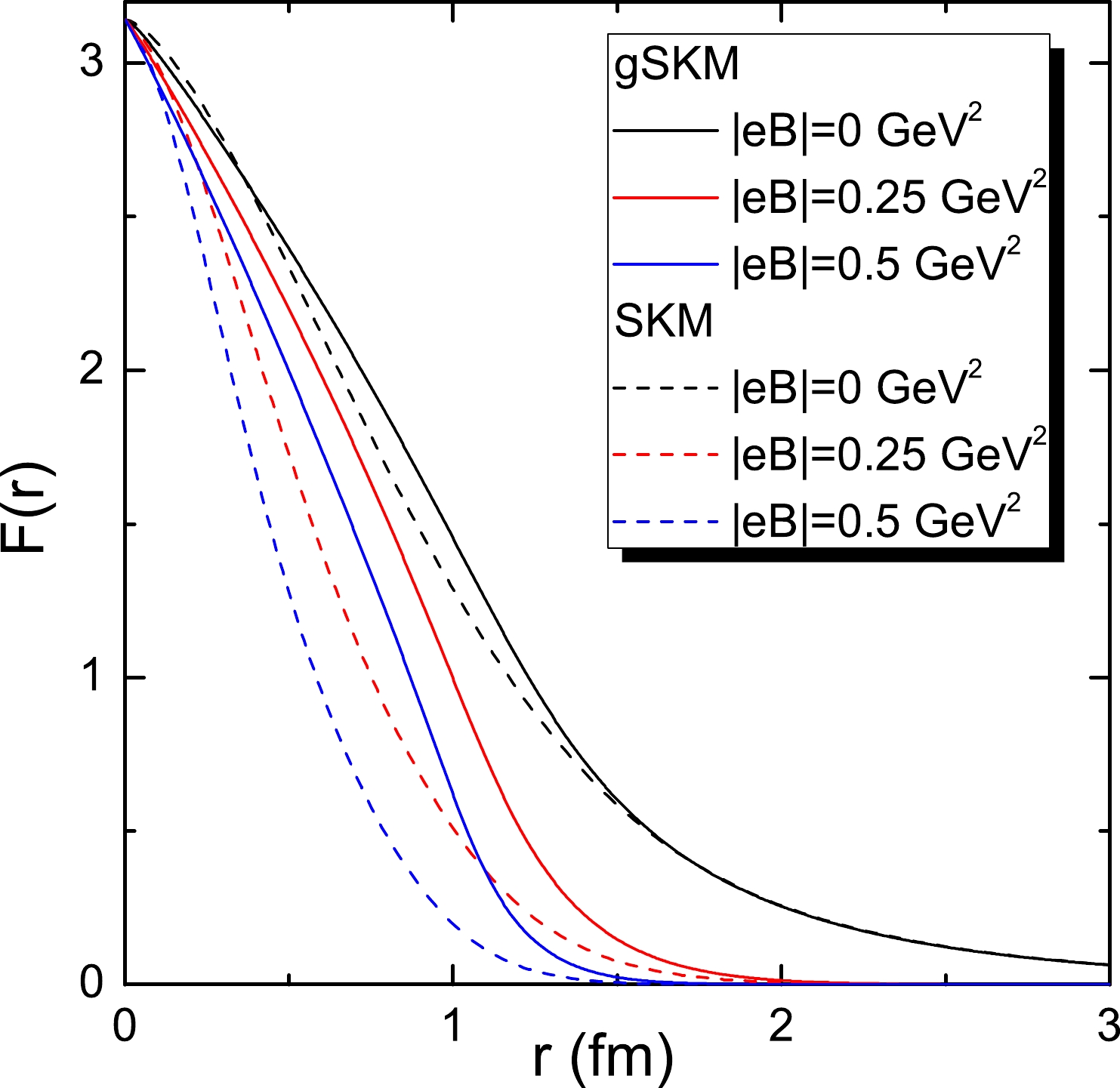
Figure 3. (color online) Profile functions
$F(r)$ for the deuteron in the ground state.In Fig. 4, we illustrate the
$ |eB| $ dependence of the mass for the deuteron. It is shown that the calculated masses in the absence of magnetic fields are 1750 and 1760 MeV for the SKM and gSKM, respectively, for the ground state$ ^3S_1 $ , and 1783 and 1798 MeV for the SKM and gSKM, respectively, for the excited state$ ^1S_0 $ (all of which are small compared with the experimental values), and 1876 and 1880 MeV for the$ ^3S_1 $ and$ ^1S_0 $ states. With increasing magnetic field strength, the calculated masses are shown to increase, and more specifically, they increase faster under the strong magnetic fields in the gSKM than in the SKM. This is mainly a result of the continuously increasing$ M_{d,st} $ , the static contribution to the deuteron mass, defined in Eq. (10), the increasing velocity with$ |eB| $ of which is larger in the gSKM. Even though the kinematical contribution$ M_{d,\rm kin} $ , defined in Eq. (22), plays a minor role, it can still be seen that in the gSKM,$ M_{d,\rm kin} $ , that is, the difference between the thick and thin curves in Fig. 4, is smaller under strong magnetic fields than that in the SKM. Physically speaking,$M_{d,\rm kin}$ can be regarded as the rotational energy in the deuteron mass, and the small kinematical energy in the gSKM can be interpreted as the large moment of inertia, which might conform with the phenomenon that$ R_x $ decreases with$ |eB| $ more slowly in the gSKM than in the SKM, as shown in Fig. 2.
Figure 4. (color online)
$|eB|$ dependence of the masses of the deuteron in the ground (color black) and excited states (color red) for the gSKM and SKM. The thin curves are only for the static contribution$M_{d,st}$ to the deuteron mass, defined in Eq. (10). The thick curves are for the deuteron mass$M_d$ , which is the sum of the static and kinematical contributions. -
In summary, we modify the method proposed in Ref. [8] to adapt to the investigation for the deuteron under strong magnetic fields. Besides the conventional Skyrme model, the effects of the derivative dependent sextic Lagrangian term are also considered. The main conclusions are listed below.
(i) The deviation of the calculated results in the presence of the magnetic fields from the cRMA, that is,
$ c_z=1 $ in this study, is$ \lesssim 10\ $ %.(ii) The phenomenon that the RMS radii decrease with increasing magnetic fields indicates a gathering of the electric charges when the magnetic fields increase.
(iii) The static contribution of the deuteron mass increases with increasing magnetic field strength, and the increasing velocity is larger for the gSKM. This results in the continuous increasing of the mass with
$ |eB| $ , which is faster for the gSKM than for the SKM. The kinematical contribution plays a minor role and is smaller under strong magnetic fields in the gSKM than that in the SKM.Unlike in Ref. [8], where only the spatial rotation in the x – y plane is considered when the skyrmion is quantized, we consider three-dimensional rotation in spatial space as well as in isospin space in this study. This quantization method can extend to the investigation of the
$ B>2 $ skyrmion under magnetic fields more conveniently than that used in Ref. [8] because both spin and isospin rotations can be considered independently, and the quantization rules for skyrmions, the so-called Finkelstein-Rubinstein constraints [28, 29], which constrain the spins and isospins of quantum states, are satisfied more easily. This method can also be used to study the$ B=1 $ skyrmion. These issues are interesting and may be explored in detail in future studies. -
The equations needed in Eqs. (17)–(19) are listed below.
$ \begin{aligned}[b]\\ a_{10}=&\int {\rm d} r \frac{\sin^2( F)}{6 c_z^2 }\left\{2[-8 + 3 \pi + c_z^3 (16-3\pi)]\sin^2( F)\right.\left.+ [32 - 9 \pi + 4 c_z^3 (-8 + 3 \pi)] r^2 F'^2+6 c_z^2 \pi r^2\right\} \\ & +\frac{\kappa\sin^4(F) F'^2}{3c_z} [-8+3 \pi + 3 c_z^3 (4 - \pi) ]\,\,, \end{aligned} \tag{A1}$ 
$ a_{11}=\int {\rm d}rr^2R_3S_3\{(4-\pi)\sin^4(F) +\frac{A}{6c_z^2}[-28 + 9 \pi + 4 c_z^3 (10 - 3 \pi)]\sin^4(F)F'^2\}\,\,, \tag{A2} $

$ \begin{aligned}[b] a_{12}=&\int {\rm d}rr^4\frac{\sin^4( F)}{24 c_z }\left\{ c_z^3 (1 - S_3^2) [30 - 58 R_3^2 + 9 \pi (-1 + 2 R_3^2)]\right. \left. - 2 (1 + S_3^2) [9 - 19 R_3^2 + \pi (-3 + 6 R_3^2)]\right\} \\ &+\frac{\kappa\sin^4(F) F'^2}{240 c_z^3}\big\{c_z^3 \{5 [-26 + 9 \pi + S_3^2 (-86 + 27 \pi)]- 2 [-139 + 45 \pi + 3 S_3^2 (-143 + 45 \pi)] R_3^2\} \\ &- 4 S_3^2 [-95 + 189 R_3^2 + \pi (30 - 60 R_3^2)] - 2 c_z^6 (-1 + S_3^2) [95 - 189 R_3^2 + 30 \pi (-1 + 2 R_3^2)]\big\}\,\,, \end{aligned}\tag{A3} $

$\begin{aligned}[b] a_{30}=&\int {\rm d}r \frac{\sin^2(F)}{3 c_z^2}\left\{6 c_z^2 r^2 (4-\pi) + 2[32 - 9 \pi\right.+ c_z^3 (-28 + 9 \pi)] \sin^2(F)+ [-28 + 9 \pi \left. + 4 c_z^3 (10 - 3 \pi)] r^2 F'^2\right\}\\&+\frac{4\kappa}{3c_z}\sin^4(F)F'^2\,\,, \end{aligned}\tag{A4} $

$ \begin{aligned}[b] a_{32}=&\int {\rm d}rr^4 \frac{\sin^4( F)}{24 c_z } (1 - R_3^2)[2 (1 + S_3^2) (10 - 3 \pi)- c_z^3 (1 - S_3^2) (28 - 9 \pi)]-\frac{\kappa\sin^4(F) F'^2}{240 c_z^3}(1 - R_3^2) \\ & \{8 S_3^2 (47 - 15 \pi) + 4 c_z^6 (-1 + S_3^2) (-47 + 15 \pi) + c_z^3 [-148 + 45 \pi + S_3^2 (-428 + 135 \pi)]\}\,\,, \end{aligned} \tag{A5}$

$ \begin{aligned}[b] b_{10}=&\int {\rm d}r \frac{2}{15 c_z^3 }\Big\{-5\sin^2(F) \big\{2 [-40 + c_z^3 (56 - 18 \pi) + 12 \pi + c_z^6 (-10 + 3 \pi)] r^2 + c_z [-64 + 18 \pi - 6 c_z^3 (-28 + 9 \pi) \\ &+ c_z^6 (-104 + 33 \pi)] \sin^2(F)\big\} +r^2F'^2 \big[2 (-1 + c_z^3)^2 r^2 + 5 c_z [-16 + c_z^3 (66 - 21 \pi) + 6 \pi + 2 c_z^6 (-28 + 9 \pi)]\\ & \sin^2(F)\big] \Big\} +\frac{\kappa\sin^4(F) F'^2}{3c_z} [8 + c_z^3 (-8 + 3 \pi) ]\,\,, \end{aligned} \tag{A6} $

$\begin{aligned}[b] b_{11}=&\int {\rm d}rr^2 R_3S_3\Big\{\frac{4}{15 c_z^3 } \sin^2(F) \big\{-5 [-96 + c_z^3(160- 51 \pi)+ 30 \pi + 3 c_z^6 (-22 + 7 \pi)] \sin^2(F) \\ &+ 2 (-1+c_z^3)^2(-47 + 15 \pi) r^2 F'^2\big\} +\frac{\kappa}{3c_z^2}[32 -9\pi+c_z^3 (-28 + 9 \pi)] \sin^4(F)F'^2\Big\}\,\,, \end{aligned} \tag{A7}$

$ \begin{aligned}[b] b_{12}=&\int {\rm d}rr^4 \frac{\sin^2( F)}{3360 c_z^4} \Big\{-14 \big\{-32 c_z^3 [330 - 1178 R_3^2 +15 \pi (-7 + 25 R_3^2)]+ 4 (1 + S_3^2) [800 - 2976 R_3^2 \\ & + 15 \pi (-17 + 63 R_3^2)] + 2 c_z^9 (-1 + S_3^2) [1840 - 5704 R_3^2 - 15 \pi (39 - 121 R_3^2)]+ c_z^6 \big[5 [2176 - 693 \pi \\ & + (-7360 + 2343 \pi) R_3^2]+ S_3^2 [45 \pi (43 - 153 R_3^2) + 64 (-95 + 338 R_3^2)]\big]\big\} \sin^2(F)+4 (-1 + c_z^3)^2\\ &\big[6 c_z^3 (-1 + S_3^2) [328 - 105 \pi + (-988 + 315 \pi) R_3^2] + (1 + S_3^2) [1656 - 4952 R_3^2 + 525 \pi (-1 + 3 R_3^2)]\big] \\& r^2 F'^2\Big\} +\frac{\kappa\sin^4(F) F'^2}{480 c_z^3} \Big\{4 c_z^9 (-1 + S_3^2) (236 - 75 \pi) (-1 + R_3^2) - 8 c_z^6 \big\{4 (-2 + S_3^2) (-47 + 15 \pi) + [-706 \\&+ S_3^2 (518 - 165 \pi) + 225 \pi] R_3^2\big\} - 4 \big[328 - 105 \pi+ (-808 + 255 \pi) R_3^2 + 3 S_3^2 (-16 + 5 \pi) (1 + 9 R_3^2)\big] \\ &- c_z^3\big\{-3536 + 8336 R_3^2 + 45 \pi (25 - 59 R_3^2) + S_3^2 [1552 - 495 \pi + (-3152 + 1005 \pi) R_3^2]\big\}\Big\}\,\,. \end{aligned} \tag{A8} $

Deuteron under strong magnetic fields: Skyrme model study
- Received Date: 2022-09-27
- Available Online: 2023-03-15
Abstract: We explore the deuteron under strong magnetic fields in Skyrme models. The effects of the derivative dependent sextic term in the Skyrme Lagrangian are investigated, and the rational map approximation is used to describe the deuteron. The influences of strong magnetic fields on the electric charge distribution and mass of the deuteron are discussed.


 DownLoad: