


 Abstract
 HTML
HTML Reference
 Related
 PDF
PDF


-
One of the main goals in the study of high energy heavy-ion collisions is to explore the QCD phase structure and critical point (CP) [1–4]. Owing to the fermion sign problem, lattice QCD calculation is restricted to the region of a vanishing or small baryon chemical potential (
$ \mu_B $ ) and predicts a crossover from the hadronic phase to a quark gluon plasma (QGP) phase in this area [5, 6]. The results of QCD based models indicate that the transition could be first-order at large$ \mu_B $ [7]. The point where the first-order phase transition ends is the CP [8, 9]. This CP is proposed to be characterized by a second-order phase transition, which becomes a unique property of strongly interacting matter [10–13]. Attempts are being made to explore the CP and phase boundary both experimentally and theoretically [10–21].The QCD equation of state with a CP is an essential ingredient for hydrodynamic simulations of fireball evolution in heavy-ion collisions. The universality of critical phenomena allows us to predict the leading singularity, i.e., the leading term of Taylor expansion, of the QCD equation of state near the CP [21]. Systems with the same symmetry in the same dimension share the same critical behaviour, even though they are governed by different interactions. It is argued that the QCD CP belongs to the same Z(2) universality class [22, 23] as the three-dimensional (3D) Ising model [1, 24–27]. Therefore, universality makes the Ising model very relevant for studies of systems that display Z(2) symmetry [28–31]. Via parameterization of the scaling equation of state in the 3D Ising model and non-universal mapping, it allows us to construct an equation of state matching the first principle lattice QCD calculations and include the proper scaling behavior in the proximity of the CP [11, 32–35]. It can also map the phase diagram of the 3D Ising model onto the one of QCD [32, 36, 37]. Thus, the CP, the lines of the first-order phase transition, and crossover in the 3D Ising model are related to those of QCD.
Classifying phases of matter and identifying phase transitions are central topics in current phase structure investigations. In the conventional statistical method, these rely on the identification of order parameters or the analysis of singularities in the free energy and its derivatives. However, the order parameter of the QCD phase transition is difficult to determine and measure in experiments. Moreover, certain phases, such as topological ones [38, 39], do not have any clear order parameters because the symmetry that drives the phase transition is not manifest in the Hamiltonian. Therefore, it is important to develop new methods of identifying phases in these systems. With the development of more powerful computers and artificial neural networks, machine learning (ML) [40, 41], a data-driven method, is proposed to be increasingly efficient for these studies. In particular, deep neural networks have been applied to recognize, classify, and characterize complex sets of data. Such methods have proved to be useful and strikingly successful for the investigation of complex physical problems [42, 43]. For example, they have been used in the study of the QCD equation of state by classifying phase transition types [44–49], in the search for the order parameter of nuclear liquid-gas phase transitions [50, 51], and in identifying phase transitions by circumventing the fermion sign problem [52]. One of the most promising advantages of deep learning is that it only requires raw low-level data, such as spin configurations in the Ising model; hence, only elementary knowledge of physics is required. With sufficiently large datasets, higher-level features can be recognized by various ML architectures [53], which can then be used to identify phases.
The last decade has witnessed several exciting explorations into identifying phase transitions in the Ising model using both supervised and unsupervised ML techniques [28, 29, 54–69]. It has been shown that the ML method is able to recognize phases and phase transitions in various two-dimensional (2D) Ising Hamiltonians [54–58]. The order parameters of multiple types of models can be learned by the weight parameters in the hidden layers of the neural networks [59–64]. This allows the statistical finite-size scaling analysis to locate the critical temperature and important critical exponents [65, 66]. Furthermore, the critical region of the Ising system can be identified, and the symmetry that drives the transition can be reconstructed from the performance of the ML process [29]. However, the majority of current investigations focus on the 2D model, and studies are restricted to only the second-order phase transition of the Ising model. A systematic investigation of the phase diagram and first-order transition of the 3D Ising model remains unexplored using ML methods.
In this study, we explore the ability of a supervised learning method to discriminate phases and classify phase transitions according to configurations produced by a 3D Ising model. We first demonstrate that deep neural networks can learn thermodynamical observables such as magnetization or energy. With a unique network architecture, they can identify both second- and first-order phase transitions in the phase diagram of the Ising model. The important features for the classification of different phases in different types of phase transitions are extracted. The rest of the paper is organized as follows. In Sec. II, we give a brief description of the 3D Ising model and its phase structure, explaining how the ML method learns the spin configurations in the model. The results of identifying different types of phase transitions in the Ising model are reported and discussed in Sec. III. Our findings are summarized in Sec. IV.
-
The Ising model [70] is regarded as one of the most fundamental magnetic models used to study the nature of phase transitions from a microscopic viewpoint in statistical physics. The energy of any particular state is given by the Ising Hamiltonian
$ \begin{array}{*{20}{l}} E=-H\sum\limits_{i}\sigma_i-J\sum\limits_{\langle ij\rangle}\sigma_i\sigma_j. \end{array} $

(1) Here,
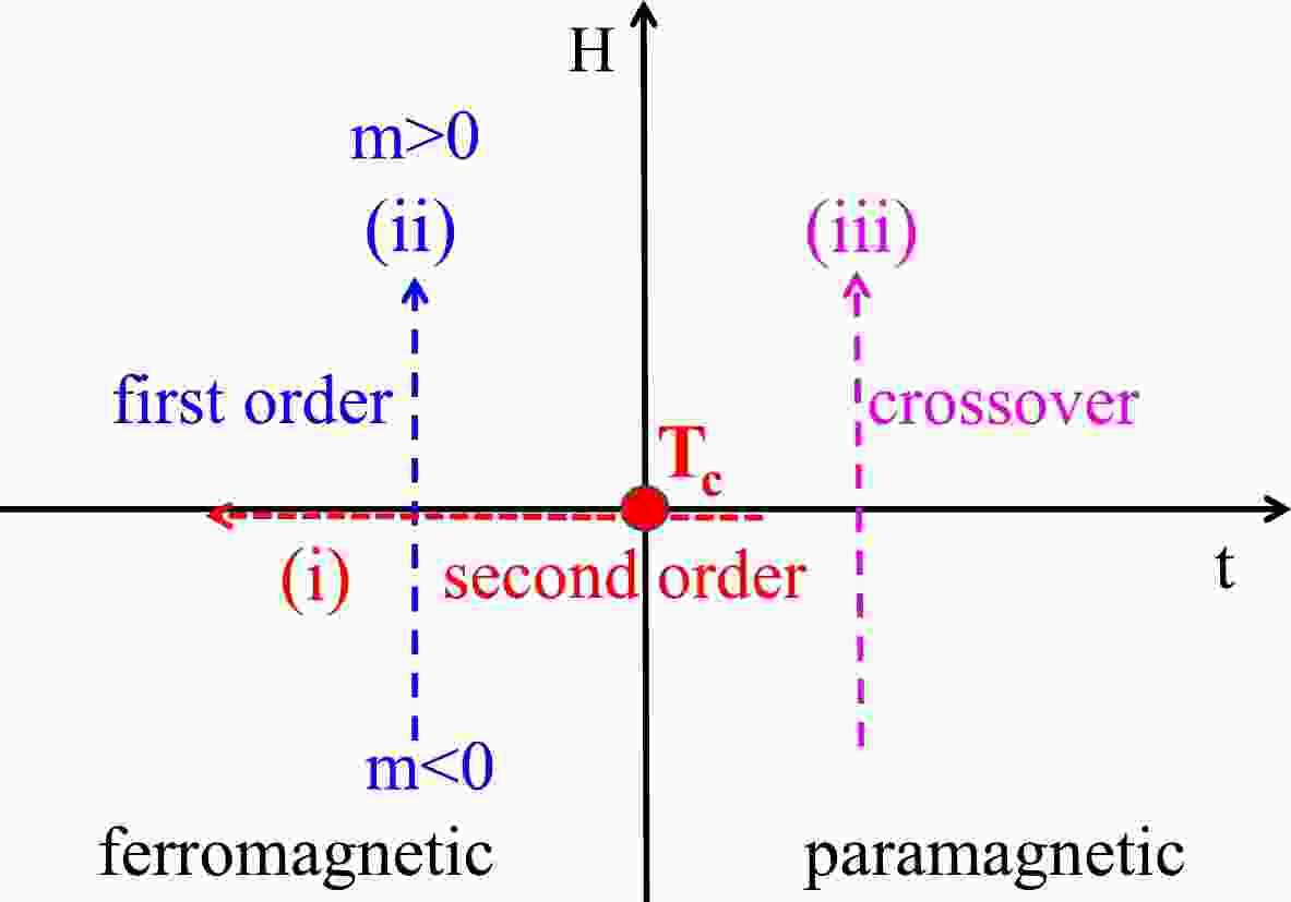
$ \sigma_i $ is the spin of the ith site. It equals either 1 (spin up) or –1 (spin down). We consider the model on a cubic lattice with periodic boundary conditions and set$ J=1 $ as the energy unit. The first sum describes the interaction of the spins with an external magnetic field H. The energy is minimum when a spin points parallel to the external magnetic field. The second sum is taken only over pairs$ (i,j) $ that are nearest neighbors in the grid, and it describes the interaction of the spins with each other. The interaction energy of a pair of adjacent spins is minimum when they point in the same direction. We usually normalize quantities of interest by the number of degrees of freedom and then work with the average energy per spin,$ \epsilon=\langle E\rangle/N $ , and the average magnetization per spin,$ m=\dfrac{1}{N}\langle\sum_{i}\sigma_i\rangle $ . The average magnetization can be regarded as the order parameter of this model.The phase diagram of the 3D Ising model [34, 37] is shown in Fig. 1. The horizontal and vertical axes in the figure are the reduced temperature
$ t=(T-T_c)/T_c $ and external magnetic field H, respectively. When decreasing the temperature under zero magnetic field, i.e., along the direction of line (i) shown in the plot, a second-order phase transition with spontaneous twofold symmetry breaking occurs at the CP$ T_c $ . A discrete Z(2) spin inversion symmetry is broken in the ferromagnetic (order) phase below$ T_c $ and is restored in the paramagnetic (disordered) phase at temperatures above$ T_c $ . On the other hand, when we change the external magnetic field with a fixed temperature below$ T_c $ , i.e., along the direction of line (ii), a first-order phase transition occurs between two phases corresponding to$ m<0 $ and$ m>0 $ . The stable phase is the one for which m has the same sign as H, but the magnetization remains nonzero even in the limit$ H\rightarrow 0 $ . The system therefore undergoes a first-order phase transition in which m changes discontinuously as it crosses the coexistence curve at$ H=0 $ . The size of the discontinuity decreases with increasing temperature and reaches zero at the critical temperature$ T_c $ , i.e., the coexistence curve ends at a CP. When we change the external magnetic field with a fixed temperature beyond$ T_c $ , i.e., along the direction of line (iii), the transition is a smooth crossover. Based on non-universal mapping between Ising variables$ (t,H) $ and QCD coordinates$ (T,\mu_B) $ in the phase diagrams, we can construct an equation of state matching the first principle lattice QCD calculations, which can be employed in hydrodynamic simulations of relativistic heavy-ion collisions [32–35].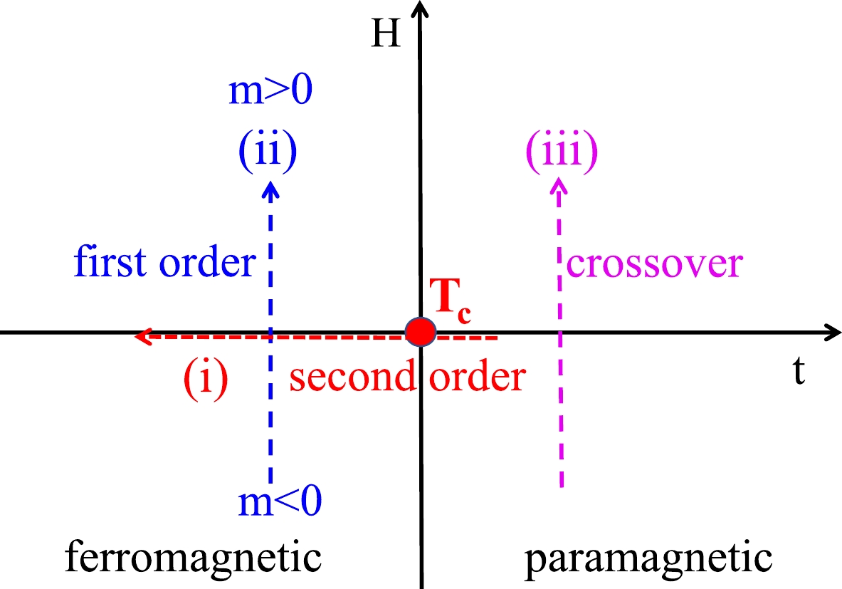
Figure 1. (color online) Phase diagram of the 3D Ising model.
A Monte Carlo (MC) simulation of the 3D Ising model on a size of
$ L\times L\times L $ is implemented via the Metropolis algorithm. This algorithm is a simple and widely used approach to generate the canonical ensemble. It allows us to efficiently obtain a large number of uncorrelated sample configurations over a wide temperature range. We generate$ 20000 $ independent spin configurations at each selected temperature and external magnetic field. Approximately$ 90 $ % of event samples are randomly chosen as inputs to train the ML model, and the rest are used to test its performance. To reduce correlations of samples, we take 50 sweeps between every two independent configurations [71].ML as a tool for identifying phase transitions has recently garnered significant attention in this field. Supervised learning, a commonly used method, is performed with a training set to teach models to yield the desired output. The algorithm measures its accuracy through the loss function, which is adjusted until the error is sufficiently minimized. After training, the neural network can recognize unseen samples and predict the correct label, illustrating that it has learned important features that can be used for classification tasks.
In deep learning, a convolutional neural network (CNN) [53] is a class of deep neural networks, mostly applied to analyze visual imagery. It is inspired by biological processes in which the connectivity pattern between neurons resembles the organization of the animal visual cortex. The CNN is known as the shift or space invariant of multilayer perceptrons for certain architectures [72]. It has the distinguishing features of local connectivity, shared weights, pooling, etc. Motivated by previous studies [54, 62, 63, 66], we apply ML techniques to the 3D Ising model. Supervised learning with a deep CNN architecture is used to explore the phase transitions and structure of the system.
-
In thermodynamics, a phase transition occurs when there is a singularity in the free energy. In the Ising model, calculations of the average energy of various spin configurations help to obtain free energy. Then, a standard recipe can be followed to find all other quantities of interest. Another important macroscopic quantity that describes the system is the average magnetization (order parameter). Phase transitions often involve the development of some type of order with associated symmetry breaking. The broken symmetry is described by an order parameter that usually increases continuously as the system moves deeper into the ordered phase and measures the degree of order as the phase transition proceeds.
A detailed schematic of the CNN architecture used in this analysis is shown in Fig. 2. The network is composed of a 4D input layer of
$ L\times L\times L\times 1 $ , two 3D convolutional layers, a pooling layer, a fully connected hidden layer, and an output layer. In addition, the pooling and fully connected hidden layers are followed by a dropout layer with a rate of 0.001 and 0.1, respectively. In the first convolutional layer, there are four filters with a size of$ 2\times 2\times 2 $ and stride$ s = 1 $ , which are applied on the input configurations and create activations. These activations are further convoluted in the second convolutional layer, which has the same number, size, and stride of filters as the first convolutional layer. The second convolutional layer is then forwarded by a pooling layer of size$ 2\times 2\times 2 $ and stride$ s=1 $ . The fully connected layer has 16 neurons, and the output layer is another fully connected layer with softmax activation and two neurons to indicate the result of classification. In this study, all the layers are activated by LeaklyReLU functions, except for the output layer. The mean-square error function is used as a loss function, and the Adam optimizer is utilized to update the weights and biases.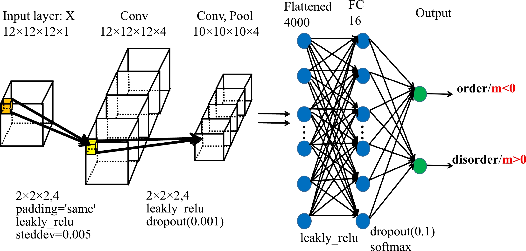
Figure 2. (color online) 3D convolutional neural network architecture used in our analysis.
We perform supervised learning for spin configurations in the 3D Ising model. The input data for ML networks are obtained from MC sampling at different magnetic fields ranging from –0.9 to 0.9 at
$ T=3.6 $ in a cubic lattice$ L = 20 $ . The spin configurations are labeled by their corresponding average magnetization or energy. The datasets are randomly divided into training and testing sets. The supervised ML networks are trained in the training sets and predicted in the testing sets. We adopt a 3D CNN architecture that is based on Tensorflow 2.0 and implemented with the Keras library.We train the 3D CNNs to predict the magnetization and energy of spin configurations and then take an average over the test sets. The results are shown in Fig. 3 (a) and (b) for average magnetization and average energy, respectively. The red circles represent the averaged predictions from the 3D CNNs, and the black squares are the calculations from MC simulations. The averaged magnetization and energy from predictions of the 3D CNNs agree well with those from the MC simulations. This means that the machine can learn physical quantities of order parameter and energy from pure spin configurations in the Ising model.
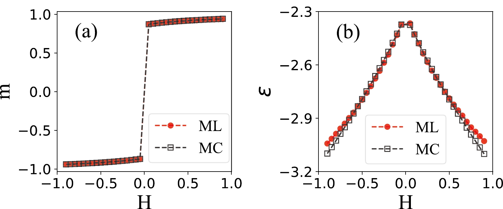
Figure 3. (color online) (a) Average magnetization and (b) average energy obtained from predictions of the 3D CNNs (red circles) and Monte Carlo simulations (black squares).
-
We now consider the ability of ML to identify phase transitions in the 3D Ising model. As described in Sec. II, the second-order phase transition of the 3D Ising model occurs at a critical temperature
$ T_c $ . It separates a ferromagnetic phase, characterized by a nonzero average magnetization per spin, from a featureless paramagnetic phase at high temperatures. For a given cubic size lattice, each sample in the MC simulations is binary labeled with its corresponding phase, i.e., the high-temperature disorder phase$ (0, 1) $ when$ T > T_c $ and the low-temperature order phase$ (1, 0) $ when$ T < T_c $ . This gives us the opportunity to attempt to classify the two different types of configurations without use of any thermodynamical estimators. The problem of identifying the phase for a certain value of temperature is then reformulated as a classification problem in ML.We construct a 3D CNN to perform supervised learning directly on the uncorrelated raw configurations sampled using MC. The numerical results obtained at various system sizes with
$ T\in (3.0,6.0) $ at a vanishing magnetic field are illustrated in Fig. 4 (a). The average outputs of different sizes cross at a certain temperature close to that obtained from Monte Carlo simulations [73, 74]. The CNN model successfully classifies the high- and low-temperature phases. The result is solely based on the raw spin configurations without providing any other thermodynamical quantities. The overall accuracies obtained from the test sets with different system sizes L are shown in Fig. 4 (c). The prediction accuracy increases from$ 86.3 $ % (for$ L=8 $ ) to$ 96.7 $ % (for$ L=28 $ ).
Figure 4. (color online) (a) Output layer averaged over test sets as a function of temperature for six different system sizes. (b) Data collapse of the average output layer as a function of
$ tL^{\frac{1}{\nu}} $ , where$ t=(T-T_c)/T_c $ is the reduced temperature. (c) Overall accuracies as a function of L.Critical exponents of the 3D Ising model are important physical quantities to describe the critical behavior of phase transitions. They are universal, i.e., they do not depend on the details of the physical system. If the CP of QCD exists, it may well be that its actual critical exponents are those of the 3D Ising model. The correlation length ξ in an infinite system near the CP is expected to diverge as
$ \xi\sim|T-T_c|^{-\nu} $ , where ν is the critical exponent of correlation length. For a finite system, one expects that the correlation length is proportionate to the system size, and thus$ |T-T_c|\sim L^{-1/\nu} $ . We perform a finite-size scaling analysis [75] to extract the critical temperature$ T_c $ and the critical exponent ν using the outputs of different sizes in$ L\in[8,28] $ . The results are shown in Fig. 4 (b). The data points of various sizes collapse with each other at$ T_c = 4.517\pm 0.003 $ and$ \nu = 0.63 \pm 0.09 $ , which agrees well with the results of$ T_c = 4.512\pm 0.001 $ and$ \nu = 0.63 \pm 0.01 $ obtained using the MC method [73, 76] and renormalization group theory [77]. Therefore, ML can not only detect phases and locate the transition temperature$ T_c $ , but also obtain the correct critical exponent of the 3D Ising model. -
The power of neural networks lies in their ability to generalize to tasks beyond their original design. In the previous subsection, we construct a 3D CNN to successfully identify the second-order phase transition in the 3D Ising model. We want to know if the same network architecture can also be used to discriminate the first-order transition in the model.
From the phase diagram of the Ising model demonstrated in Fig. 1, the first-order phase transition occurs when we change the external magnetic field H across the transition boundary
$ H=0 $ with$ T<T_c $ . To study the effect of temperature on this transition, we generate event samples by taking two different temperatures of$ T=3.6 $ (far from the critical temperature$ T_c $ ) and$ T=4.5 $ (near$ T_c $ ). The same 3D CNN architecture as illustrated in Fig. 2 is used to train and make predictions on the test sets for both cases within the range$ H\in [-0.2, 0.2] $ . The results are shown in Fig. 5 (a) and (b), respectively. The CNN architecture, which is originally constructed to identify the second-order phase transition, can also successfully classify the$ m<0 $ and$ m>0 $ phases. The average outputs of three different sizes cross exactly at$ H=0 $ in both cases. The test accuracies with different system sizes are shown in Fig. 5 (c). When the temperature of the system is far from$ T_c $ , the network can classify phases perfectly (blue dots). The accuracy decreases with decreasing system size when the temperature is near$ T_c $ (red triangles). This is due to the effect of large critical fluctuations when the system is near the temperature where the second-order phase transition occurs.
Figure 5. (color online) Output layer averaged over test sets as a function of external magnetic field for three different system sizes at (a) T = 3.6 and (b) T = 4.5. (c) The overall accuracies as a function of L at two different temperatures.
-
In statistical physics, the second-order phase transition is a continuous transition, whereas the first-order phase transition is a discontinuous one. They belong to different types of phase transitions and have different equations of state. The great advantage of the DL method is the ability to extract hidden features automatically from a dataset without the need for human intervention. The neural network should itself select appropriate features within the data that are most sensitive to the properties of different types of equations of state. To obtain physical insights into how the neural-network discriminates the phase transitions in the Ising model, it is useful to visualize the complex dependence learned by the network. DL uses multiple layers of representation to learn descriptive features directly from training data. The important features, which are used in the classification process for phase transitions and for identifying any underlying physical quantities, may be encoded in convolutional filter kernels [78], weight matrices [62, 64, 78], or the activations of hidden units in the network [79]. The sets of variational parameters, specifically the weights and biases at each layer of the neural network, are optimized during the training process. They will converge to certain values, which encode the solution to the particular problem under consideration.
We observe that a uniform network architecture can identify different phases in either the second-order or first-order phase transitions in the 3D Ising model. It is interesting to find out which quantities can possibly be used for the classification processes in the results of Fig. 4 and 5. Figure 6 shows a scatter plot of the outputs for two neurons in the final output layer of the CNN with magnetization, the absolute value of magnetization, and energy. From the first row for the second-order phase transition, we find that the outputs of the network are proportional to the absolute value of magnetization and energy rather than the magnetization of the input configurations. The calculated absolute values of the Pearson correlation coefficients are 0.17, 0.93, and 0.85 for Fig. 6 (a), (b), and (c), respectively. As for the second row for the first-order transition, the outputs of the network are found to be proportional to magnetization rather than the absolute value of magnetization or energy. The absolute values of the Pearson correlation coefficients are 1, 0.1, and 0.08 for Fig. 6 (d), (e), and (f), respectively.

Figure 6. (color online) Correlations between the outputs of two neurons in the output layer of the neural network and magnetization (a)(d), the absolute value of magnetization (b)(e), and energy (c)(f). The first row represents the result from the second-order phase transition, and the second row is that from the first-order phase transition.
Within the shallow layers of a network architecture, the variational parameters correspond to learned universal features. This form of universality is diminished toward deeper layers, where the features are expected to transit from universal to specific in relation to different systems. The activation function of a variable in an intermediate layer of the neural network acts as a transformation that maps a certain input to an output representation [79].
We calculate the mean activation functions of neural network configurations of different phases with
$ L = 12 $ in the second- and first-order phase transitions. The results are shown in Fig. 7, where the activations are drawn for 16 neurons of the fully connected layer. The blue and green bars represent the calculations from different phases in the same transitions. The maximum value is normalized to one, and the results are rescaled accordingly for better representation. In Fig. 7 (a), we observe that nearly all of the 16 neurons for both the order and disorder phases are activated in the second-order phase transition, although the values of the two phases are different from each other. This may be due to large fluctuations near the CP in this transition. This might also be reminiscent of the connection between DL and the renormalization group [67, 80]. As for the first-order phase transition in Fig. 7 (b), it is found that different phases ($ m<0 $ and$ m>0 $ ) activate different neurons.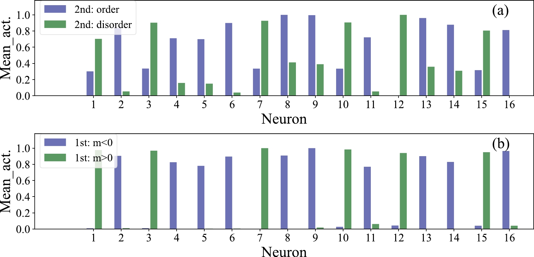
Figure 7. (color online) Mean activations of the 16 hidden neurons in the fully connected layer of the 3D Ising-trained convolutional neural network of different phases in the second-order (a) and first-order (b) phase transitions.
-
In this paper, we employ a supervised learning method to study phase transitions in the 3D Ising model. It is found that a 3D CNN can be trained to predict the magnetization and energy of spin configurations. The network successfully classifies the high- and low-temperature phases of the 3D Ising model. It is able to not only locate the transition temperature but also obtain the critical exponent of the second-order phase transition based on raw spin configurations using the finite-size scaling analysis method. With the same CNN architecture, the neural network can identify different phases in the first-order transition with high accuracy. This implies that the network captures both the second- and first-order phase transitions and encodes them in the parameters of the network during the process of supervised learning. Furthermore, we attempt to extract and decode important features of the classification processes directly from the data. It is found that the neural network detects phases by the absolute value of magnetization and energy in the second-order phase transition, whereas it tends to rely on magnetization in the first-order transition. The calculated mean activations in the high-level representations show that almost all the neurons before the output layer are activated in the second-order phase transition, but different phases activate different neurons in the case of the first-order.
In relativistic heavy-ion collisions, we expect the QCD CP to have similar critical behaviors to those in the 3D Ising model owing to the same universality that is dictated by the symmetry of the systems. In heavy-ion experiments, the measured high-order cumulants [15, 81, 82] and intermittency [83–86] both at SPS and RHIC energies suggest that there are large density fluctuations near the QCD CP. Here, we prove that the state-of-the-art ML method can learn important features that discriminate different phases in the phase transition. Understanding what this approach captures will be useful when we experimentally explore the QCD CP and phase boundary. The method developed in this study can also be applied to investigate the criticality in MC models, which could help to explore the physical mechanisms of the QCD phase transition.
-
We are grateful to Prof. Longgang Pang and Mingmei Xu for their fruitful discussions and comments. We further thank Prof. Hengtong Ding for providing us with computing resources. The numerical simulations have been performed on the GPU cluster in the Nuclear Science Computing Center at Central China Normal University (NSC3).
X. L. and R. G. contributed equally to this study.
Machine learning phase transitions of the three-dimensional Ising universality class
- Received Date: 2022-07-20
- Available Online: 2023-03-15
Abstract: Exploration of the QCD phase diagram and critical point is one of the main goals in current relativistic heavy-ion collisions. The QCD critical point is expected to belong to a three-dimensional (3D) Ising universality class. Machine learning techniques are found to be powerful in distinguishing different phases of matter and provide a new way to study the phase diagram. We investigate phase transitions in the 3D cubic Ising model using supervised learning methods. It is found that a 3D convolutional neural network can be trained to effectively predict physical quantities in different spin configurations. With a uniform neural network architecture, it can encode phases of matter and identify both second- and first-order phase transitions. The important features that discriminate different phases in the classification processes are investigated. These findings can help study and understand QCD phase transitions in relativistic heavy-ion collisions.


 DownLoad: