


 Abstract
 HTML
HTML Reference
 Related
 PDF
PDF


-
Since the discovery of
$ X(3872) $ by Belle in 2003 [1], many charmonium-like$ XYZ $ states have been discovered [2]. Some of these structures may contain four quarks,$ \bar c c \bar q q $ ($ q=u/d $ ), and are therefore good candidates for hidden-charm tetraquark states.In recent years, the LHCb Collaboration has continuously observed as many as five interesting exotic structures:
● In 2015, the LHCb experiment observed two structures,
$ P_c(4380)^+ $ and$ P_c(4450)^+ $ , in the$ J/\psi p $ invariant mass spectrum of the$ \Lambda_b^0\to J/\psi p K^- $ decays [3]:$ \begin{aligned}[b] P_c(4380)^+: M=& 4380 \pm 8 \pm 29 \rm{ MeV} \, ,\\ \Gamma=& 205 \pm 18 \pm 86 \rm{ MeV} \, , \end{aligned} $

(1) $ \begin{aligned}[b] P_c(4450)^+: M=& 4449.8 \pm 1.7 \pm 2.5 \rm{ MeV} \, , \\ \Gamma=& 39 \pm 5 \pm 19 \rm{ MeV} \, . \end{aligned} $

(2) This observation was later supported by a subsequent LHCb experiment investigating the
$ J/\psi p $ invariant mass spectrum of the$ \Lambda_b^0\to J/\psi p \pi^- $ decays [4].● In 2019, the LHCb experiment observed a new structure,
$ P_c(4312)^+ $ , and further separated$ P_c(4450)^+ $ into two substructures,$ P_c(4440)^+ $ and$ P_c(4457)^+ $ , again in the$ J/\psi p $ invariant mass spectrum of the$ \Lambda_b^0\to J/\psi p K^- $ decays [5].$ \begin{aligned}[b] P_c(4312)^+: M=& 4311.9 \pm 0.7 ^{+6.8}_{-0.6} \rm{ MeV} \, , \\ \Gamma=& 9.8 \pm 2.7 ^{+3.7}_{-4.5} \rm{ MeV} \, , \end{aligned} $

(3) $ \begin{aligned}[b] P_c(4440)^+: M=& 4440.3 \pm 1.3 ^{+4.1}_{-4.7} \rm{ MeV} \, ,\\ \Gamma=& 20.6 \pm 4.9 ^{+8.7}_{-10.1} \rm{ MeV} \, , \end{aligned} $

(4) $ \begin{aligned}[b] P_c(4457)^+: M=& 4457.3 \pm 0.6 ^{+4.1}_{-1.7} \rm{ MeV} \, ,\\ \Gamma=& 6.4 \pm 2.0 ^{+5.7}_{-1.9} \rm{ MeV} \, .\\ \end{aligned} $

(5) ● In 2020, the LHCb experiment reported evidence of a hidden-charm pentaquark state with strangeness,
$ P_{cs}(4459)^0 $ , in the$ J/\psi \Lambda $ invariant mass spectrum of the$ \Xi_b^- \to J/\psi \Lambda K^- $ decays [6].$ \begin{aligned}[b] P_{cs}(4459)^0: M=& 4458.8 \pm 2.9^{+4.7}_{-1.1} \rm{ MeV} \, , \\ \Gamma=& 17.3 \pm 6.5^{+8.0}_{-5.7} \rm{ MeV} \, . \end{aligned} $

(6) These structures contain at least five quarks,
$ \bar c c u u d $ or$ \bar c c u d s $ ; therefore, they are perfect candidates for hidden-charm pentaquark states. The charmonium-like$ XYZ $ and hidden-charm pentaquark states have attracted significant attention, and studies on these states have greatly improved our understanding of the non-perturbative behaviors of the strong interaction in the low energy region [7–18].To understand the
$ P_c $ and$ P_{cs} $ states, various theoretical interpretations have been proposed, such as loosely-bound hadronic molecular states [19–40], tightly-bound compact pentaquark states [41–51], and kinematical effects [52–55]. In particular, the three narrow states$ P_c(4312)^+ $ ,$ P_c(4440)^+ $ , and$ P_c(4457)^+ $ are just below the$ \bar D \Sigma_c $ and$ \bar D^{*} \Sigma_c $ thresholds; therefore, it is natural to describe them as$ \bar D^{(*)} \Sigma_c $ hadronic molecular states, whose existence was predicted in Refs. [56–60] before the 2015 LHCb experiment [3]. The other narrow state,$ P_{cs}(4459)^0 $ , is just below the$ \bar D^{*} \Xi_c $ threshold; hence, it is natural to describe it as the$ \bar D^{*} \Xi_c $ molecular state [61, 62].However, these exotic structures were only observed in the LHCb experiment [3–6]. It is crucial to search for their partner states as well as other potential decay channels to further understand their nature. There have been several theoretical studies on this subject using, for example, effective approaches [63–66], the quark interchange model [67, 68], heavy quark symmetry [69, 70], and QCD sum rules [71]. We refer to reviews [7–18] and the references therein for detailed discussions.
In this paper, we systematically investigate hidden-charm pentaquark states as
$ \bar D^{(*)} \Sigma_c^{(*)} $ hadronic molecular states through their corresponding hidden-charm pentaquark interpolating currents. We systemically construct all the relevant currents and apply QCD sum rules to calculate their masses and decay constants. The obtained results are used to further study their production and decay properties.Our strategy is fairly straightforward. First, we construct a hidden-charm pentaquark current, such as
$ \begin{aligned}[b] \sqrt2 \xi_1(x) =& [\delta^{ab} \bar c_a(x) \gamma_5 d_b(x)] \\ & \times [\epsilon^{cde} u_c^T(x) \mathbb{C} \gamma_\mu u_d(x) \gamma^\mu \gamma_5 c_e(x)] \, , \end{aligned} $

(7) where
$ a \cdots e $ are color indices. This is the best coupling of the current to the$ D^- \Sigma_c^{++} $ molecular state of$ J^P = 1/2^- $ through$ \langle 0 | \xi_1 | D^- \Sigma_c^{++}; 1/2^-(q) \rangle = f_1 u(q) \, , $

(8) where
$ u(q) $ is the Dirac spinor of$ | D^- \Sigma_c^{++}; 1/2^- \rangle $ . Its decay constant$ f_1 $ can be calculated using QCD sum rules.Second, we investigate three-body
$ \Lambda_b^0 \to J/\psi p K^- $ decays. The total quark content of the final states is$ udc \bar c s \bar u u $ , where the intermediate states$ D^{(*)-} \Sigma_c^{(*)++} K^- $ can be produced. We apply Fierz rearrangement to carefully examine the combination of these seven quarks, from which we select the current$ \xi_1 $ and evaluate the relative production rate of$ | D^- \Sigma_c^{++}; 1/2^- \rangle $ .Third, we apply the Fierz rearrangement of the Dirac and color indices to transform the current
$ \xi_1 $ into$ \sqrt2 \xi_1 \rightarrow {1\over6} \; [\bar c_a \gamma_5 c_a]\; N - {1\over12} \; [\bar c_a \gamma_\mu c_a]\; \gamma^\mu \gamma_5 N + \cdots \, , $

(9) where
$ N = \epsilon^{abc} (u_a^T \mathbb{C} d_b) \gamma_5 u_c - \epsilon^{abc} (u_a^T \mathbb{C} \gamma_5 d_b) u_c $ is Ioffe's light baryon field coupling to a proton [72–74]. Accordingly,$ \xi_1 $ couples to the$ \eta_c p $ and$ J/\psi p $ channels simultaneously:$ \begin{aligned}[b] \langle 0 | \xi_1 | \eta_c p \rangle \approx& {\sqrt2\over12} \langle 0 | \bar c_{a} \gamma_5 c_a | \eta_c \rangle\; \langle 0 | N | p \rangle + \cdots \, , \\ \langle 0 | \xi_1 | \psi p \rangle \approx & -{\sqrt2\over24} \langle 0 | \bar c_{a} \gamma_\mu c_a | \psi \rangle\; \gamma^\mu \gamma_5 \langle 0 | N | p \rangle + \cdots \, . \end{aligned} $

(10) We can use these two equations to straightforwardly calculate the relative branching ratio of the
$ | D^- \Sigma_c^{++}; 1/2^- \rangle $ decay into$ \eta_c p $ to its decay into$ J/\psi p $ [75]. We refer to Ref. [76] for detailed discussions. There, we applied the same method to study the decay properties of$ P_c(4312)^+ $ ,$ P_c(4440)^+ $ , and$ P_c(4457)^+ $ as$ \bar D^{(*)} \Sigma_c $ molecular states, and in this paper, we apply it to study the decay properties of the$ \bar D^{(*)} \Sigma_c^* $ molecular states.This paper is organized as follows. In Sec. II, we systematically construct the hidden-charm pentaquark currents corresponding to the
$ \bar D^{(*)} \Sigma_c^{(*)} $ hadronic molecular states. We use them to perform QCD sum rule analyses in Sec. III and calculate their masses and decay constants. The obtained results are used in Sec. IV to study their production in$ \Lambda_b^0 $ decays using current algebra. In Sec. V, we use the Fierz rearrangement of the Dirac and color indices to study the decay properties of the$ \bar D^{(*)} \Sigma_c^{*} $ molecular states and calculate several of their relative branching ratios. The obtained results are summarized and discussed in Sec. VI. -
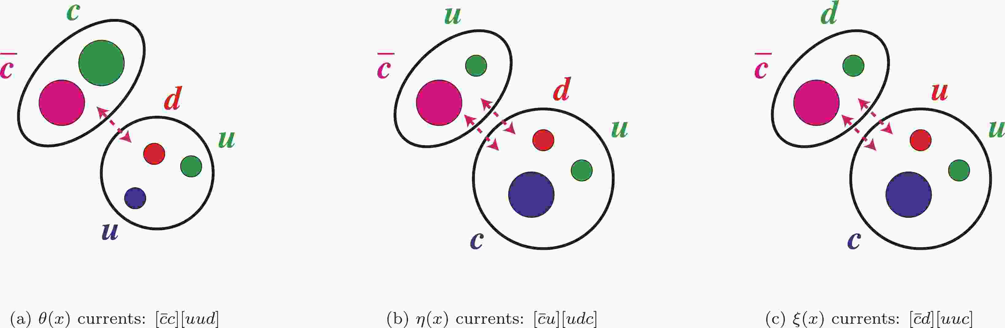
In this section, we use the
$ \bar c $ , c, u, u, and d ($ q=u/d $ ) quarks to construct hidden-charm pentaquark interpolating currents. We consider the following three types of currents:$ \begin{aligned}[b] \theta(x) =& [\bar c_a(x) \Gamma^\theta_1 c_b(x)] \; \Big[[q^T_c(x) \mathbb{C} \Gamma^\theta_2 q_d(x)] \; \Gamma^\theta_3 q_e(x)\Big] \, , \\ \eta(x) =& [\bar c_a(x) \Gamma^\eta_1 u_b(x)] \; \Big[[u^T_c(x) \mathbb{C} \Gamma^\eta_2 d_d(x)] \; \Gamma^\eta_3 c_e(x) \Big] \, ,\\ \xi(x) =& [\bar c_a(x) \Gamma^\xi_1 d_b(x)] \; \Big[[u^T_c(x) \mathbb{C} \Gamma^\xi_2 u_d(x)] \; \Gamma^\xi_3 c_e(x) \Big] \, , \end{aligned} $

(11) where
$ a \cdots e $ are color indices,$ \Gamma_{1/2/3}^{\theta/\eta/\xi} $ are Dirac matrices, and$ \mathbb{C} = {\rm i}\gamma_2 \gamma_0 $ is the charge-conjugation operator. We illustrate these in Fig. 1. These three configurations can be related using Fierz rearrangement in Lorentz space and color rearrangement.
Figure 1. (color online) Three types of hidden-charm pentaquark interpolating currents,
$\theta(x)$ ,$\eta(x)$ , and$\xi(x)$ . Quarks are shown in red/green/blue, and antiquarks are shown in cyan/magenta/yellow. Taken from Ref. [76].$ \delta^{ab} \epsilon^{cde} = \delta^{ac} \epsilon^{bde} + \delta^{ad} \epsilon^{cbe} + \delta^{ae} \epsilon^{cdb} \, . $

(12) This is discussed in detail in Sec. V, where we construct the
$ \theta(x) $ currents by combining charmonium operators and light baryon fields.In this section, we construct the
$ \eta(x) $ and$ \xi(x) $ currents and use them to construct currents corresponding to the$ \bar D^{(*)} \Sigma_c^{(*)} $ hadronic molecular states. To achieve this, we combine charmed meson operators and charmed baryon fields. There are five independent charmed meson operators:$\begin{aligned}[b]& \quad\quad\quad\quad\quad \bar c_a q_a \, [0^+] \, , \quad \, \bar c_a \gamma_5 q_a \, [0^-] \, ,\quad\\&\bar c_a \gamma_\mu q_a \, [1^-] \, ,\quad \, \bar c_a \gamma_\mu \gamma_5 q_a \, [1^+] \, , \,\quad \bar c_a \sigma_{\mu\nu} q_a \, [1^\pm] \, .\end{aligned} $

(13) There is another,
$ \bar c_d \sigma_{\mu\nu} \gamma_5 q_d $ ; however, it is related to$ \bar c_d \sigma_{\mu\nu} q_d $ through$ \sigma_{\mu\nu} \gamma_5 = {{\rm i}\over2} \epsilon_{\mu\nu\rho\sigma} \sigma^{\rho\sigma} \, . $

(14) In particular, we require the
$ J^P = 0^- $ and$ 1^- $ operators to construct the$ \eta(x) $ and$ \xi(x) $ currents, which couple to the ground-state charmed mesons$ {\cal{D}} = D/D^{*} $ .$ J_{D} = \bar c_a \gamma_5 q_a \, , \quad J_{D^{*}} = \bar c_a \gamma_\mu q_a \, . $

(15) Charmed baryon fields have been systematically constructed and studied in Refs. [77–80] using the method of QCD sum rules [81, 82] within heavy quark effective theory [83–85]. In this paper, we require the following charmed baryon fields,
$ J_{{\cal{B}}} $ , which couple to the ground-state charmed baryons$ {\cal{B}} = \Lambda_c/\Sigma_c/\Sigma_c^{*} $ :$ \begin{aligned}[b] J_{\Lambda_c^+} =& \epsilon^{abc} [u_a^T \mathbb{C} \gamma_{5} d_b] c_c \, , \\ \sqrt2 J_{\Sigma_c^{++}} =& \epsilon^{abc} [u_a^T \mathbb{C} \gamma_{\mu} u_b] \gamma^{\mu}\gamma_{5} c_c \, , \\ J_{\Sigma_c^+} =& \epsilon^{abc} [u_a^T \mathbb{C} \gamma_{\mu} d_b] \gamma^{\mu}\gamma_{5} c_c \, , \\ \sqrt2 J_{\Sigma_c^{0}} =& \epsilon^{abc} [d_a^T \mathbb{C} \gamma_{\mu} d_b] \gamma^{\mu}\gamma_{5} c_c \, , \\ \sqrt2 J^\alpha_{\Sigma_c^{*++}} =& \epsilon^{abc} P_{3/2}^{\alpha\mu} [u_a^T \mathbb{C} \gamma_{\mu} u_b] c_c \, , \\ J^\alpha_{\Sigma_c^{*+}} =& \epsilon^{abc} P_{3/2}^{\alpha\mu} [u_a^T \mathbb{C} \gamma_{\mu} d_b] c_c \, , \\ \sqrt2 J^\alpha_{\Sigma_c^{*0}} =& \epsilon^{abc} P_{3/2}^{\alpha\mu} [d_a^T \mathbb{C} \gamma_{\mu} d_b] c_c \, . \end{aligned} $

(16) Here,
$ P_{3/2}^{\mu\nu} $ is the spin-3/2 projection operator$ P_{3/2}^{\mu\nu} = g^{\mu\nu} - {1 \over 4} \gamma^\mu\gamma^\nu \, . $

(17) In the molecular picture,
$ P_c(4312)^+ $ ,$ P_c(4440)^+ $ , and$ P_c(4457)^+ $ are usually interpreted as the$ \bar D \Sigma_c $ and$ \bar D^* \Sigma_c $ hadronic molecular states [20, 21, 60]. Their relevant currents have been constructed in Ref. [76]. In this paper, we further construct the$ \bar D \Sigma_c^{*} $ and$ \bar D^* \Sigma_c^{*} $ currents; they are all summarized here for completeness.Altogether, there can be seven
$ \bar D^{(*)} \Sigma_c^{(*)} $ hadronic molecular states, which are$ \bar D \Sigma_c $ of$J^P = {1/2}^-$ ,$ \bar D^* \Sigma_c $ of$ J^P = {(1/2)}^-/{(3/2)}^- $ ,$ \bar D \Sigma_c^* $ of$J^P = {3/2}^-$ , and$ \bar D^* \Sigma_c^* $ of$J^P = {(1/2)}^-/{(3/2)}^-/{(5/2)}^-$ :$\begin{aligned}[b] | \bar D \Sigma_c; {1/2}^- ; \theta \rangle =& \cos\theta\; | \bar D^0 \Sigma_c^+;1/2^- \rangle\\& + \sin\theta\; | D^- \Sigma_c^{++};1/2^- \rangle \, , \end{aligned}$

(18) $\begin{aligned}[b] | \bar D^* \Sigma_c; {1/2}^- ; \theta \rangle =& \cos\theta\; | \bar D^{*0} \Sigma_c^+;1/2^- \rangle \\&+ \sin\theta\; | D^{*-} \Sigma_c^{++};1/2^- \rangle \, , \end{aligned}$

(19) $ \begin{aligned}[b] | \bar D^* \Sigma_c; {3/2}^- ; \theta \rangle =& \cos\theta\; | \bar D^{*0} \Sigma_c^+;3/2^- \rangle \\&+ \sin\theta\; | D^{*-} \Sigma_c^{++};3/2^- \rangle \, , \end{aligned} $

(20) $\begin{aligned}[b] | \bar D \Sigma_c^*; {3/2}^- ; \theta \rangle =& \cos\theta\; | \bar D^{0} \Sigma_c^{*+};3/2^- \rangle \\&+ \sin\theta\; | D^- \Sigma_c^{*++};3/2^- \rangle \, , \end{aligned} $

(21) $\begin{aligned}[b] | \bar D^* \Sigma_c^*; {1/2}^- ; \theta \rangle =& \cos\theta\; | \bar D^{*0} \Sigma_c^{*+};1/2^- \rangle \\&+ \sin\theta\; | D^{*-} \Sigma_c^{*++};1/2^- \rangle \, ,\end{aligned}$

(22) $\begin{aligned}[b] | \bar D^* \Sigma_c^*; {3/2}^- ; \theta \rangle =& \cos\theta\; | \bar D^{*0} \Sigma_c^{*+};3/2^- \rangle \\&+ \sin\theta\; | D^{*-} \Sigma_c^{*++};3/2^- \rangle \, , \end{aligned} $

(23) $ \begin{aligned}[b] | \bar D^* \Sigma_c^*; {5/2}^- ; \theta \rangle =& \cos\theta\; | \bar D^{*0} \Sigma_c^{*+};5/2^- \rangle\\& + \sin\theta\; | D^{*-} \Sigma_c^{*++};5/2^- \rangle \, , \end{aligned} $

(24) where θ is an isospin parameter satisfying
$ \theta = -55^{\rm{o}} $ for$ I=1/2 $ and$ \theta = 35^{\rm{o}} $ for$ I=3/2 $ . In the present study, we concentrate on the former$ I=1/2 $ states, so that we may simplify the notations to$ \begin{aligned}[b] | \bar D^{(*)} \Sigma_c^{(*)}; J^P \rangle =& {\sqrt{1/3}}\; | \bar D^{(*)0} \Sigma_c^{(*)+}; J^P \rangle \\&- {\sqrt{2/3}}\; | D^{(*)-} \Sigma_c^{(*)++}; J^P \rangle . \end{aligned} $

(25) Their relevant interpolating currents are
$ J_i = \cos\theta\; \eta_i + \sin\theta\; \xi_i \, , $

(26) where
$ \begin{aligned}[b] \eta_1 =& [\delta^{ab} \bar c_a \gamma_5 u_b] \; [\epsilon^{cde} u_c^T \mathbb{C} \gamma_\mu d_d \gamma^\mu \gamma_5 c_e] \\ =& \bar D^0 \; \Sigma_c^+ \, , \end{aligned} $

(27) $ \begin{aligned}[b] \eta_2 =& [\delta^{ab} \bar c_a \gamma_\nu u_b] \; \gamma^\nu \gamma_5 \; [\epsilon^{cde} u_c^T \mathbb{C} \gamma_\mu d_d \gamma^\mu \gamma_5 c_e] \\ =& \bar D^{*0}_\nu \; \gamma^\nu \gamma_5 \; \Sigma_c^+ \, , \end{aligned} $

(28) $ \begin{aligned}[b] \eta_3^\alpha =& P_{3/2}^{\alpha\nu} \; [\delta^{ab} \bar c_a \gamma_\nu u_b] \; [\epsilon^{cde} u_c^T \mathbb{C} \gamma_\mu d_d \gamma^\mu \gamma_5 c_e] \\ =& P_{3/2}^{\alpha\nu} \; \bar D^{*0}_\nu \; \Sigma_c^+ \, , \end{aligned} $

(29) $ \begin{aligned}[b] \eta_4^\alpha =& [\delta^{ab} \bar c_a \gamma_5 u_b] \; P_{3/2}^{\alpha\mu} [\epsilon^{cde} u_c^T \mathbb{C} \gamma_\mu d_d c_e] \\ =& \bar D^0 \; \Sigma_c^{*+;\alpha} \, , \end{aligned} $

(30) $ \begin{aligned}[b] \eta_5 =& [\delta^{ab} \bar c_a \gamma_\nu u_b] \; P_{3/2}^{\nu\mu} [\epsilon^{cde} u_c^T \mathbb{C} \gamma_\mu d_d c_e] \\ =& \bar D^{*0}_\nu \; \Sigma_c^{*+;\nu} \, , \end{aligned} $

(31) $ \begin{aligned}[b] \eta_6^{\alpha} =& [\delta^{ab} \bar c_a \gamma_\nu u_b] \; P_{3/2}^{\alpha\rho} \; \gamma^\nu \gamma_5 \; P^{3/2}_{\rho\mu} [\epsilon^{cde} u_c^T \mathbb{C} \gamma^\mu d_d c_e] \\ =& \bar D^{*0}_\nu \; P_{3/2}^{\alpha\rho} \; \gamma^\nu \gamma_5 \; \Sigma_{c;\rho}^{*+} \, , \end{aligned} $

(32) $ \begin{aligned}[b] \eta_7^{\alpha\beta} =& P^{\alpha\beta,\nu\rho}_{5/2} \; [\delta^{ab} \bar c_a \gamma_\nu u_b] \; P^{3/2}_{\rho\mu} [\epsilon^{cde} u_c^T \mathbb{C} \gamma^\mu d_d c_e] \\ =& P^{\alpha\beta,\nu\rho}_{5/2} \; \bar D^{*0}_\nu \; \Sigma_{c;\rho}^{*+} \, , \end{aligned} $

(33) and
$ \begin{aligned}[b] \xi_1 =& {1\over\sqrt2} \; [\delta^{ab} \bar c_a \gamma_5 d_b] \; [\epsilon^{cde} u_c^T \mathbb{C} \gamma_\mu u_d \gamma^\mu \gamma_5 c_e] \\ =& D^- \; \Sigma_c^{++} \, , \end{aligned} $

(34) $ \begin{aligned}[b] \xi_2 =& {1\over\sqrt2} \; [\delta^{ab} \bar c_a \gamma_\nu d_b] \; \gamma^\nu \gamma_5 \; [\epsilon^{cde} u_c^T \mathbb{C} \gamma_\mu u_d \gamma^\mu \gamma_5 c_e] \\ =& D^{*-}_\nu \; \gamma^\nu \gamma_5 \; \Sigma_c^{++} \, , \end{aligned} $

(35) $ \begin{aligned}[b] \xi_3^\alpha =& {1\over\sqrt2} \; P_{3/2}^{\alpha\nu} \; [\delta^{ab} \bar c_a \gamma_\nu d_b] \; [\epsilon^{cde} u_c^T \mathbb{C} \gamma_\mu u_d \gamma^\mu \gamma_5 c_e] \\ =& P_{3/2}^{\alpha\nu} \; D^{*-}_\nu \; \Sigma_c^{++} \, , \end{aligned} $

(36) $ \begin{aligned}[b] \xi_4^\alpha =& {1\over\sqrt2} \; [\delta^{ab} \bar c_a \gamma_5 d_b] \; P_{3/2}^{\alpha\mu} [\epsilon^{cde} u_c^T \mathbb{C} \gamma_\mu u_d c_e] \\ =& D^- \; \Sigma_c^{*++;\alpha} \, , \end{aligned} $

(37) $ \begin{aligned}[b] \xi_5 =& {1\over\sqrt2} \; [\delta^{ab} \bar c_a \gamma_\nu d_b] \; P_{3/2}^{\nu\mu} [\epsilon^{cde} u_c^T \mathbb{C} \gamma_\mu u_d c_e] \\ =& D^{*-}_\nu \; \Sigma_c^{*++;\nu} \, , \end{aligned} $

(38) $ \begin{aligned}[b] \xi_6^{\alpha} =& {1\over\sqrt2} \; [\delta^{ab} \bar c_a \gamma_\nu d_b] \; P_{3/2}^{\alpha\rho} \gamma^\nu \gamma_5 \; P^{3/2}_{\rho\mu} [\epsilon^{cde} u_c^T \mathbb{C} \gamma^\mu u_d c_e] \\ =& D^{*-}_\nu \; P_{3/2}^{\alpha\rho} \; \gamma^\nu \gamma_5 \; \Sigma_{c;\rho}^{*++} \, ,\\[-10pt] \end{aligned} $

(39) $ \begin{aligned}[b] \xi_7^{\alpha\beta} =& {1\over\sqrt2} \; P^{\alpha\beta,\nu\rho}_{5/2} \; [\delta^{ab} \bar c_a \gamma_\nu d_b] \; P^{3/2}_{\rho\mu} [\epsilon^{cde} u_c^T \mathbb{C} \gamma^\mu u_d c_e] \\ =& P^{\alpha\beta,\nu\rho}_{5/2} \; D^{*-}_\nu \; \Sigma_{c;\rho}^{*++} \, . \\[-10pt]\end{aligned} $

(40) In the above expressions, we use
$ {\cal{D}} $ and$ {\cal{B}} $ to denote the charmed meson operators$ J_{{\cal{D}}} $ and charmed baryon fields$ J_{{\cal{B}}} $ for simplicity;$ P_{5/2}^{\mu\nu,\rho\sigma} $ is the spin-5/2 projection operator$ \begin{aligned}[b] P_{5/2}^{\mu\nu,\rho\sigma} =& {1\over2} g^{\mu\rho} g^{\nu\sigma} + {1\over2} g^{\mu\sigma} g^{\nu\rho} - {1 \over 6} g^{\mu\nu} g^{\rho\sigma} - {1 \over 12} g^{\mu\rho} \gamma^{\nu}\gamma^{\sigma}\\& - {1 \over 12} g^{\mu\sigma} \gamma^{\nu}\gamma^{\rho} - {1 \over 12} g^{\nu\sigma} \gamma^{\mu}\gamma^{\rho} - {1 \over 12} g^{\nu\rho} \gamma^{\mu}\gamma^{\sigma} \, . \end{aligned} $

(41) -
In this section, we use QCD sum rules [81, 82] to study
$ \bar D^{(*)} \Sigma_c^{(*)} $ molecular states through the currents$ J_{1\cdots7} $ , that is,$ J_{1,2,5} $ of$ J^P = 1/2^- $ ,$ J^\alpha_{3,4,6} $ of$ J^P = 3/2^- $ , and$ J_{7}^{\alpha\beta} $ of$ J^P = 5/2^- $ . We calculate their masses and decay constants, and the obtained results are used in the next section to further calculate their relative production rates. Several of these calculations have been performed in Refs. [19, 86–88], and we refer to Refs. [38–40, 50, 61] for more relevant QCD sum rule studies. -
We assume that the currents
$ J_{1\cdots7} $ couple to the$ \bar D^{(*)} \Sigma_c^{(*)} $ molecular states$ X_{1\cdots7} $ through$ \begin{aligned}[b] \langle 0 | J_{1,2,5} | X_{1,2,5}; 1/2^- \rangle =& f_{X_{1,2,5}} u (p) \, , \\ \langle 0 | J_{3,4,6}^\alpha | X_{3,4,6}; 3/2^- \rangle =& f_{X_{3,4,6}} u^\alpha (p) \, , \\ \langle 0 | J_{7}^{\alpha\beta} | X_{7}; 5/2^- \rangle =& f_{X_7} u^{\alpha\beta} (p) \, , \end{aligned} $

(42) where
$ u(p) $ ,$ u^\alpha(p) $ , and$ u^{\alpha\beta}(p) $ are spinors of$ X_{1\cdots7} $ . The two-point correlation functions extracted from these currents can be written as$ \begin{aligned}[b] \Pi_{1,2,5}\left(q^2\right) =& {\rm i} \int {\rm d}^4x {\rm e}^{{\rm i}q\cdot x} \langle 0 | T\left[J_{1,2,5}(x) \bar J_{1,2,5}(0)\right] | 0 \rangle \\ =& (\not q + M_{X_{1,2,5}}) \; \Pi_{1,2,5}\left(q^2\right) \, ,\\[-10pt] \end{aligned} $

(43) $ \begin{aligned}[b] \Pi^{\alpha \alpha^\prime}_{3,4,6}\left(q^2\right) =& {\rm i} \int {\rm d}^4x {\rm e}^{{\rm i}q\cdot x} \langle 0 | T\left[J^{\alpha}_{3,4,6}(x) \bar J^{\alpha^\prime}_{3,4,6}(0)\right] | 0 \rangle \\ =& {\cal{G}}_{3/2}^{\alpha \alpha^\prime} (\not q + M_{X_{3,4,6}})\; \Pi_{3,4,6}\left(q^2\right) \, , \\[-8pt]\end{aligned} $

(44) $ \begin{aligned}[b] \Pi^{\alpha \beta,\alpha^\prime \beta^\prime}_7\left(q^2\right) =& {\rm i} \int {\rm d}^4x {\rm e}^{{\rm i}q\cdot x} \langle 0 | T\left[J^{\alpha \beta}_7(x) \bar J^{\alpha^\prime \beta^\prime}_7(0)\right] | 0 \rangle \\ =& {\cal{G}}_{5/2}^{\alpha \beta,\alpha^\prime \beta^\prime} (\not q + M_{X_7})\; \Pi_7\left(q^2\right) \, , \end{aligned} $

(45) where
$ {\cal{G}}_{3/2}^{\mu\nu} $ and${\cal{G}}_{5/2}^{\mu \nu,\,\rho \sigma}$ are coefficients of the spin-3/2 and spin-5/2 propagators, respectively.$ {\cal{G}}_{3/2}^{\mu\nu}(p) = g^{\mu\nu} - {1\over3} \gamma^\mu \gamma^\nu - {p^\mu\gamma^\nu - p^\nu\gamma^{\mu} \over 3m} - {2p^{\mu}p^\nu \over 3m^2} \, , $

(46) $ \begin{aligned}[b] {\cal{G}}_{5/2}^{\mu \nu,\rho \sigma}(p) =& \frac{1}{2}(g^{\mu\rho}g^{\nu\sigma}+g^{\mu\sigma}g^{\nu\rho}) - \frac{1}{5}g^{\mu\nu}g^{\rho\sigma} \\ &- \frac{1}{10}(g^{\mu\rho}\gamma^\nu\gamma^\sigma + g^{\mu\sigma}\gamma^\nu\gamma^\rho + g^{\nu\rho}\gamma^\mu\gamma^\sigma + g^{\nu\sigma}\gamma^\mu\gamma^\rho) \end{aligned} $

$ \begin{aligned}[b] &+ \frac{1}{10m}\Bigl(g^{\mu\rho}(p^\nu\gamma^\sigma - p^\sigma\gamma^\nu) + g^{\mu\sigma}(p^\nu\gamma^\rho - p^\rho\gamma^\nu) \\ & + g^{\nu\rho}(p^\mu\gamma^\sigma - p^\sigma\gamma^\mu) + g^{\nu\sigma}(p^\mu\gamma^\rho - p^\rho\gamma^\mu)\Bigr) \\ &+ \frac{1}{5m^2}(g^{\mu\nu}p^\rho p^\sigma + g^{\rho\sigma}p^\mu p^\nu) \\ &- \frac{2}{5m^2}(g^{\mu\rho}p^\nu p^\sigma + g^{\mu\sigma}p^\nu p^\rho + g^{\nu\rho}p^\mu p^\sigma + g^{\nu\sigma}p^\mu p^\rho) \\ &+ \frac{1}{10m^2}\Bigl(\gamma^\mu p^\nu (\gamma^\rho p^\sigma + \gamma^\sigma p^\rho) + \gamma^\nu p^\mu (\gamma^\rho p^\sigma + \gamma^\sigma p^\rho)\Bigl) \\ &+ \frac{1}{5m^3}\Bigl(p^\rho p^\sigma (\gamma^\mu p^\nu + \gamma^\nu p^\mu ) - p^\mu p^\nu (\gamma^\rho p^\sigma + \gamma^\sigma p^\rho ) \Bigl) \\ &+ \frac{2}{5m^4}p^\mu p^\nu p^\rho p^\sigma \, . \end{aligned} $

(47) In the above expressions, we assume that the states
$ X_{1\cdots7} $ have the same spin-parity quantum numbers as the currents$ J_{1\cdots7} $ so that we may use the "non-$ \gamma_5 $ coupling" in Eq. (42). Conversely, we must use the "$ \gamma_5 $ coupling,"$ \langle 0 | J_{1\cdots7} | X_{1\cdots7}^\prime \rangle = f_{X^\prime_{1\cdots7}} \gamma_5 u (p) \, , $

(48) if the states
$ X^\prime_{1\cdots7} $ have an opposite parity to the currents$ J_{1\cdots7} $ . We may alternatively use the partner currents$ \gamma_5 J_{1\cdots7} $ , which also have opposite parity.$ \langle 0 | \gamma_5 J_{1\cdots7} | X_{1\cdots7} \rangle = f_{X_{1\cdots7}} \gamma_5 u (p) \, . $

(49) From Eqs. (48) and (49), we can derive another "non-
$ \gamma_5 $ coupling" between$ \gamma_5 J_{1\cdots7} $ and$ X^\prime_{1\cdots7} $ , expressed as$ \langle 0 | \gamma_5 J_{1\cdots7} | X_{1\cdots7}^\prime \rangle = f_{X^\prime_{1\cdots7}} u (p) \, . $

(50) We refer to Refs. [89–92] for detailed discussions.
The two-point correlation functions derived from Eqs. (48) and (49) are similar to Eqs. (43)–(45) but with
$ (\not q + M_{X}) $ replaced by$ (- \not q + M_{X}) $ . Based on this feature, we can extract the parities of$ X_{1\cdots7} $ ; we use the terms proportional to$ \bf 1 $ to evaluate the masses of$ X_{1\cdots7} $ , which are then compared with the terms proportional to$ \not q $ to extract their parities.In QCD sum rule studies, we must calculate the two-point correlation function
$ \Pi\left(q^2\right) $ at both the hadron and quark-gluon levels. At the hadron level, we use the dispersion relation to express this as$ \Pi(q^2)={\frac{1}{\pi}}\int^\infty_{s_<}\frac{{\rm{Im}} \Pi(s)}{s-q^2-{\rm i}\varepsilon}{\rm d}s \, , $

(51) with
$ s_< $ the physical threshold. We define the imaginary part of the correlation function as the spectral density$ \rho(s) $ , which can be evaluated at the hadron level by inserting the intermediate hadron states$ \sum_n|n\rangle\langle n| $ as follows:$ \begin{aligned}[b] \rho_{\rm{phen}}(s) \equiv& {\rm{Im}}\Pi(s)/\pi \\ =& \sum_n\delta(s-M^2_n)\langle 0|\eta|n\rangle\langle n|{\eta^\dagger}|0\rangle \\ =& f_X^2\delta(s-m_X^2)+ \rm{continuum}. \end{aligned} $

(52) In the last step, we adopt typical parametrization of one-pole dominance for the ground state X along with a continuum contribution.
At the quark-gluon level, we calculate
$ \Pi\left(q^2\right) $ using the method of operator product expansion (OPE) and extract its corresponding spectral density$ \rho_{\rm{OPE}}(s) $ . After performing the Borel transformation at both the hadron and quark-gluon levels, we approximate the continuum using the spectral density above a threshold value$ s_0 $ (quark-hadron duality) and arrive at the sum rule equation$ \Pi(s_0, M_{\rm B}^2) \equiv f^2_X {\rm e}^{-M_X^2/M_{\rm B}^2} = \int^{s_0}_{s_<} {\rm e}^{-s/M_{\rm B}^2}\rho_{\rm{OPE}}(s){\rm d}s \, . $

(53) This can be used to further calculate
$ M_X $ and$ f_X $ through$ M^2_X(s_0, M_{\rm B}) = \frac{\displaystyle\int^{s_0}_{s_<} {\rm e}^{-s/M_{\rm B}^2}s\rho_{\rm{OPE}}(s){\rm d}s}{\displaystyle\int^{s_0}_{s_<} {\rm e}^{-s/M_{\rm B}^2}\rho_{\rm{OPE}}(s){\rm d}s} \, , $

(54) $ f_X^2(s_0, M_{\rm B}) = {\rm e}^{(M_X^2(s_0, M_{\rm B}))/ M_{\rm B}^2} \int^{s_0}_{s_<} {\rm e}^{-s/M_{\rm B}^2}\rho_{\rm{OPE}}(s){\rm d}s \, . $

(55) In this study, we calculate OPEs at the leading order of
$ \alpha_s $ and up to the$ D({\rm{imension}}) = 10 $ terms, including the perturbative term, charm quark mass, quark condensate$ \langle \bar q q \rangle $ ,gluon condensate$ \langle g_s^2 GG \rangle $ , quark-gluon mixed condensate$ \langle g_s \bar q \sigma G q \rangle $ , and their combinations$ \langle \bar q q \rangle^2 $ ,$ \langle \bar q q \rangle\langle g_s \bar q \sigma G q \rangle $ ,$ \langle \bar q q \rangle^3 $ , and$ \langle g_s \bar q \sigma G q \rangle^2 $ . We summarize the obtained spectral densities$ \rho_{1\cdots7}(s) $ in Appendix A, which are extracted from the currents$ J_{1\cdots7} $ , respectively.In these calculations, we ignore chirally suppressed terms with light quark masses and adoptthe factorization assumption of vacuum saturation for higher dimensional condensates, that is,
$ \langle (\bar q q)^2 \rangle = \langle \bar q q \rangle^2 $ ,$ \langle (\bar q q) (g_s \bar q \sigma G q) \rangle = \langle \bar q q \rangle\langle g_s \bar q \sigma G q \rangle $ ,$ \langle (\bar q q)^3 \rangle = \langle \bar q q \rangle^3 $ , and$ \langle (g_s \bar q \sigma G q)^2 \rangle = \langle g_s \bar q \sigma G q \rangle^2 $ . We find that the$ D=3 $ quark condensate$ {\langle\bar qq\rangle} $ and the$ D=5 $ mixed condensate$ \langle g_s \bar q \sigma G q \rangle $ are both multiplied by the charm quark mass$ m_c $ and are thus important power corrections.In the following subsection, we use the spectral densities
$ \rho_{1\cdots7}(s) $ to perform numerical analyses and calculate the masses and decay constants of$ X_{1\cdots7} $ . First, however, let us investigate the current$ J_1 $ as an example. This has the quantum number$ J^P = 1/2^- $ and couples to the$ \bar D \Sigma_c $ molecular state$ X_1 $ . Its spectral density$ \rho_1(s) $ is given in Eq. (A1). We find that the terms multiplied by$ m_c $ are almost positively proportional to the terms multiplied by$ \not q $ . Hence, the extracted parity of$ X_1 $ is found to be negative, which is the same as$ J_1 $ . In other words,$ J_1 $ mainly couples to a negative-parity state. Similarly, all the$ \bar D^{(*)} \Sigma_c^{(*)} $ molecular states defined in Eqs. (18)–(24) are found to have negative parity. -
In this subsection, we use the spectral densities
$ \rho_{1\cdots7}(s) $ extracted from the currents$ J_{1\cdots7} $ to perform numerical analyses and calculate the masses and decay constants of$ X_{1\cdots7} $ . As discussed in the previous subsection, we only use the terms proportional to$ m_c $ to achieve this.We use the current
$ J_1 $ as an example, whose spectral density$ \rho_1(s) $ can be found in Eq. (A1), and apply the following QCD sum rule parameter values [93–101]:$ \begin{aligned}[b] m_c=& 1.275 ^{+0.025}_{-0.035} \rm{ GeV} \, , \\ \langle \bar qq \rangle =& - (0.24 \pm 0.01)^3 \rm{ GeV}^3 \, , \\ \langle g_s^2GG\rangle =& (0.48 \pm 0.14) \rm{ GeV}^4\, , \\ \langle g_s \bar q \sigma G q \rangle =& M_0^2 \times \langle \bar qq \rangle\, , \\ M_0^2 =& (0.8 \pm 0.2) \rm{ GeV}^2 \, , \end{aligned} $

(56) where the running mass in the
$ \overline{MS} $ scheme is used for the charm quark.There are two free parameters in Eqs. (54) and (55), the Borel mass
$ M_{\rm B} $ and threshold value$ s_0 $ . We use two criteria to constrain the Borel mass$ M_{\rm B} $ for a fixed$ s_0 $ . The first criterion is to ensure the convergence of the OPE series. This is achieved by requiring the$ D=10 $ terms ($ m_c \langle \bar q q \rangle^3 $ and$ \langle g_s \bar q \sigma G q \rangle^2 $ ) to be less than 10% so that the lower limit of$ M_{\rm B} $ can be determined.$ \rm{Convergence} \equiv \left|\frac{ \Pi^{D=10}(\infty, M_{\rm B}) }{ \Pi(\infty, M_{\rm B}) }\right| \leq 10\% \, . $

(57) We show this function in Fig. 2 using the solid curve and find that OPE convergence improves with increasing
$ M_{\rm B} $ . This criterion leads to$ \left(M_{\rm B}^{\rm min}\right)^2 = 3.27 $ GeV2 when setting$ s_0 = 24 $ GeV$ ^2 $ .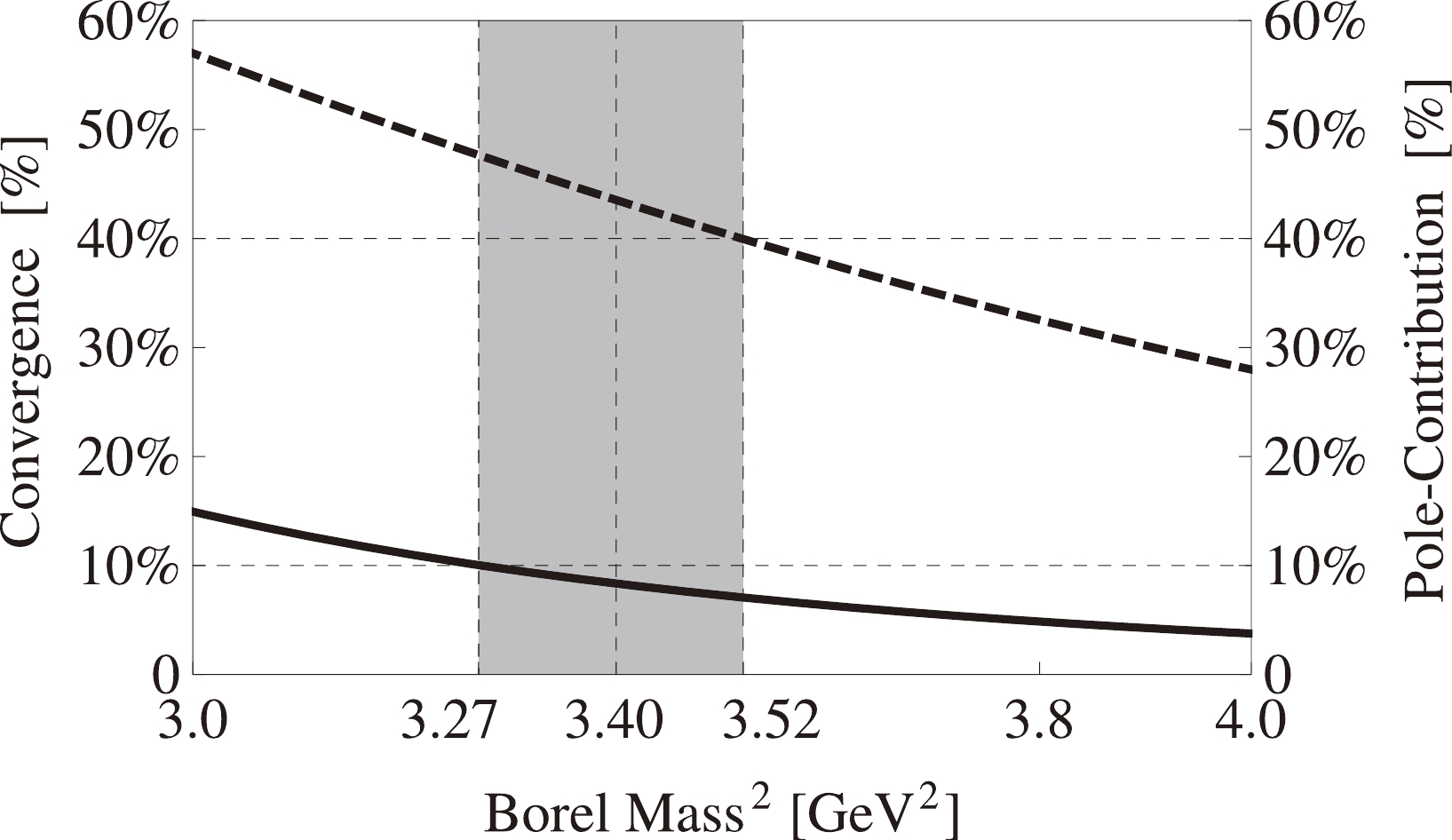
Figure 2. Convergence (solid curve, defined in Eq. (57)) and pole-contribution (dashed curve, defined in Eq. (58)) as functions of the Borel mass
$ M_{\rm B} $ . These curves are obtained using the current$ J_1 $ when setting$ s_0 = 24 $ GeV$ ^2 $ .The second criterion is to ensure the validity of one-pole parametrization. This is achieved by requiring the pole contribution to be larger than 40% so that the upper limit of
$ M_{\rm B} $ can be determined.$ \rm{Pole-Contribution} \equiv \frac{ \Pi(s_0, M_{\rm B}) }{ \Pi(\infty, M_{\rm B}) } \geq 40\% \, . $

(58) We show this function in Fig. 2 using the dashed curve and find that it decreases with increasing
$ M_{\rm B} $ . This criterion leads to$ \left(M_{\rm B}^{\rm max}\right)^2 = 3.52 $ GeV$ ^2 $ when setting$ s_0 = 24 $ GeV$ ^2 $ .Altogether, we extract the working region of the Borel mass to be
$ 3.27 $ $ < M_{\rm B}^2 < 3.52 $ GeV$ ^2 $ for the current$ J_1 $ with the threshold value$ s_0 = 24 $ GeV$ ^2 $ . We show variations in$ M_{X_1} $ and$ f_{X_1} $ with respect to the Borel mass$ M_{\rm B} $ in Fig. 3. They are shown in a broader region,$ 3.0 $ $ \leq M_{\rm B}^2 \leq 4.0 $ GeV$ ^2 $ , and are more stable inside the above Borel window.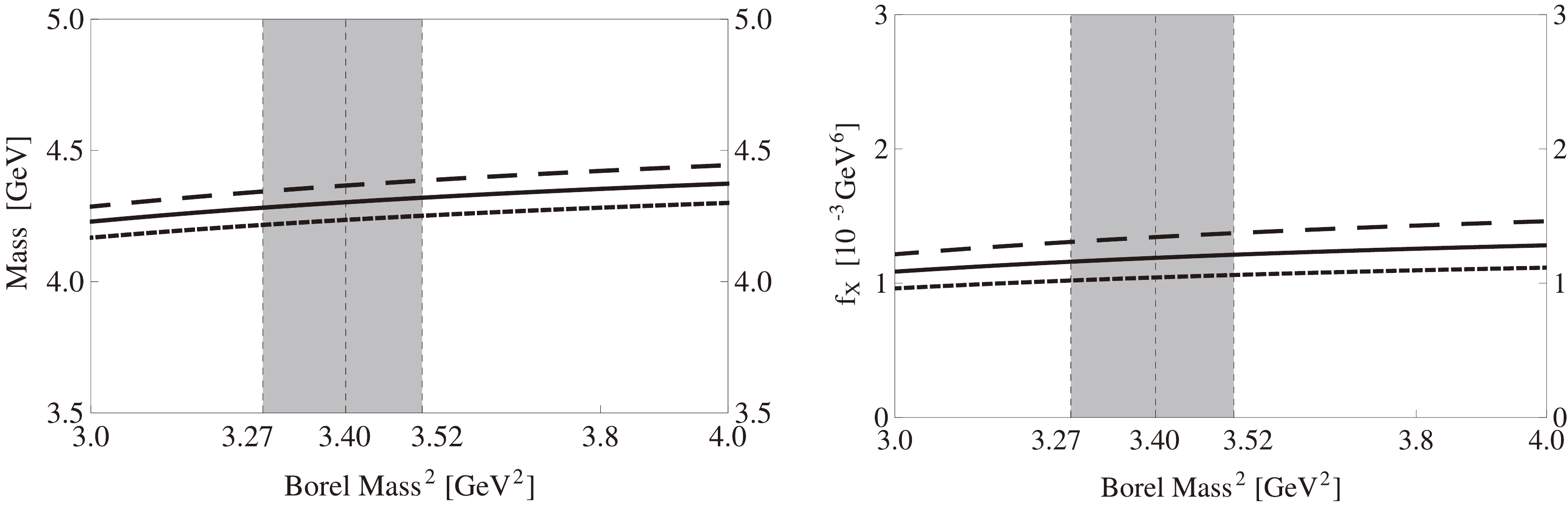
Figure 3. Variations in the mass
$M_{X}$ (left) and decay constant$f_{X}$ (right) with respect to the Borel mass$M_{\rm B}$ , calculated using the current$J_1$ . In both panels, the short-dashed, solid, and long-dashed curves are obtained by setting$s_0 = 23$ ,$24$ , and$25$ GeV$^2$ , respectively.Redoing the same procedures by changing
$ s_0 $ , we find that there are non-vanishing Borel windows as long as$ s_0 \geq s_0^{\rm min} = 22.4 $ GeV$ ^2 $ . Accordingly, we choose$ s_0 $ to be slightly larger with an uncertainty of$ \pm1.0 $ GeV, that is,$ s_0 = 24.0 \pm 1.0 $ GeV$ ^2 $ . Overall, our working regions for the current$ J_1 $ are determined to be$ 23.0 $ $ \leq s_0\leq 25.0 $ GeV$ ^2 $ and$ 3.27 $ $ \leq M_{\rm B}^2 \leq 3.52 $ GeV$ ^2 $ , for which we calculate the mass and decay constant of$ X_1 $ to be$ \begin{aligned}[b] M_{X_1} =& 4.30^{+0.10}_{-0.10} \rm{ GeV} \, , \\ f_{X_1} =& \left(1.19^{+0.19}_{-0.18}\right) \times 10^{-3} \rm{ GeV}^6 \, . \end{aligned} $

(59) Here, the central values correspond to
$ M_{\rm B}^2=3.40 $ GeV$ ^2 $ and$ s_0 = 24.0 $ GeV$ ^2 $ . Their uncertainties originate from the threshold value$ s_0 $ , Borel mass$ M_{\rm B} $ , charm quark mass$ m_c $ , and various QCD sum rule parameters listed in Eq. (56). This mass value is consistent with the experimental mass of$ P_c(4312)^+ $ [5], revealing it to be the$ I = 1/2 \bar D \Sigma_c $ molecular state of$ J^P=1/2^- $ .Similarly, we use the spectral densities
$ \rho_{2\cdots7}(s) $ extracted from the currents$ J_{2\cdots7} $ to perform numerical analyses and calculate the masses and decay constants of$ X_{2\cdots7} $ . In particular, the sum rule results extracted from the currents$ J_6^\alpha $ and$ J_7^{\alpha\beta} $ are$ \begin{aligned}[b] M_{X_6} =& 4.64^{+0.10}_{-0.10} \rm{ GeV} \, , \quad f_{X_6} = \left(1.01^{+0.15}_{-0.14}\right) \times 10^{-3} \rm{ GeV}^6 \, , \\ M_{X_7} =& 4.64^{+0.14}_{-0.12} \rm{ GeV} \, , \quad f_{X_7} = \left(0.77^{+0.12}_{-0.11}\right) \times 10^{-3} \rm{ GeV}^6 \, . \end{aligned} $

(60) These two mass values are both close to, but slightly larger than, the
$ \bar D^* \Sigma_c^* $ threshold at$ M_{D^*} + M_{\Sigma_c^*} = 4527 $ MeV. To obtain a better description of the$ \bar D^* \Sigma_c^* $ molecular states that may lie just below the$ \bar D^* \Sigma_c^* $ threshold, we loosen the criterion given in Eq. (57) to$ \rm{Convergence} \equiv \left|\frac{ \Pi^{D=10}(\infty, M_{\rm B}) }{ \Pi(\infty, M_{\rm B}) }\right| \leq 15\% \, . $

(61) Now, the masses and decay constants extracted from the currents
$ J_6^\alpha $ and$ J_7^{\alpha\beta} $ are modified to be$ \begin{aligned}[]b M^\prime_{X_6} =& 4.52^{+0.11}_{-0.11} \rm{ GeV} \, , \quad f^\prime_{X_6} = \left(0.85^{+0.14}_{-0.13}\right) \times 10^{-3} \rm{ GeV}^6 \, , \\ M^\prime_{X_7} =& 4.55^{+0.15}_{-0.13} \rm{ GeV} \, , \quad f^\prime_{X_7} = \left(0.65^{+0.11}_{-0.10}\right) \times 10^{-3} \rm{ GeV}^6 \, . \end{aligned} $

(62) Moreover, the mass of
$ |\bar D \Sigma_c^*; 3/2^- \rangle $ is calculated to be$ 4.43^{+0.10}_{-0.10} $ GeV, which is consistent with, but also slightly larger than, the$ \bar D \Sigma_c^* $ threshold at$ M_{D} + M_{\Sigma_c^*} = 4385 $ MeV. All these divergences indicate that the accuracy of our QCD sum rule results is moderate but not good enough to extract the binding energies of the$ \bar D^{(*)} \Sigma_c^{(*)} $ molecular states. Therefore, our results can suggest but not determine a) whether these$ \bar D^{(*)} \Sigma_c^{(*)} $ molecular states exist, and b) whether they are bound or resonance states. However, in this study, we are more concerned with the ratios, that is, the relative production rates and relative branching ratios, whose uncertainties can be significantly reduced. Accordingly, the decay constants$ f_X $ calculated in this section are input parameters that are more important than the masses$ M_X $ . Note that the decay constants$ f_X $ can also be used within the QCD sum rule method to directly calculate the partial decay widths through the three-point correlation functions; however, we do not perform this in the present study.We summarize all the above sum rule results in Table 1. Our results are consistent with those of Ref. [102], where the authors applied the same QCD sum rule method to study both the
$ I=1/2 \bar D^{(*)} \Sigma_c^{(*)} $ and$ I=3/2 $ molecular states. Our results support the interpretations of$ P_c(4440)^+ $ and$ P_c(4457)^+ $ [5] as the$ I = 1/2 \bar D^* \Sigma_c $ molecular states of$ J^P=1/2^- $ and$ 3/2^- $ . Again, the accuracy of our sum rule results is not good enough to distinguish or identify them. To better understand them, we study their production and decay properties in the following sections, where we find that$ P_c(4440)^+ $ and$ P_c(4457)^+ $ can be better interpreted in our framework as$ |\bar D^{*} \Sigma_c; 3/2^- \rangle $ and$ |\bar D^{*} \Sigma_c; 1/2^- \rangle $ , respectively.Currents Configuration $s_0^{\rm min}$ 

/${\rm{GeV}}^2$ 

Working regions Pole (%) Mass/GeV $f_X$ /GeV

$^6$ 

Candidate $s_0/{\rm{GeV} }^2$ 

$M_{\rm B}^2/{\rm{GeV} }^2$ 

$J_1$ 

$|\bar D \Sigma_c; 1/2^- \rangle$ 

22.4 $24.0\pm1.0$ 

$3.27$ –

$3.52$ 

$40$ –

$48$ 

$4.30^{+0.10}_{-0.10}$ 

$\left(1.19^{+0.19}_{-0.18}\right) \times 10^{-3}$ 

$P_c(4312)^+$ 

$J_2$ 

$|\bar D^* \Sigma_c; 1/2^- \rangle$ 

25.5 $27.0\pm1.0$ 

$3.78$ –

$3.99$ 

$40$ –

$46$ 

$4.48^{+0.10}_{-0.10}$ 

$\left(2.24^{+0.34}_{-0.30}\right) \times 10^{-3}$ 

$P_c(4457)^+$ 

$J_3$ 

$|\bar D^* \Sigma_c; 3/2^- \rangle$ 

24.6 $26.0\pm1.0$ 

$3.51$ –

$3.72$ 

$40$ –

$46$ 

$4.46^{+0.11}_{-0.10}$ 

$\left(1.15^{+0.18}_{-0.16}\right) \times 10^{-3}$ 

$P_c(4440)^+$ 

$J_4$ 

$|\bar D \Sigma_c^*; 3/2^- \rangle$ 

24.2 $25.0\pm1.0$ 

$3.33$ –

$3.45$ 

$40$ –

$44$ 

$4.43^{+0.10}_{-0.10}$ 

$\left(0.65^{+0.11}_{-0.10}\right) \times 10^{-3}$ 

$J_5$ 

$|\bar D^* \Sigma_c^*; 1/2^- \rangle$ 

26.0 $27.0\pm1.0$ 

$3.43$ –

$3.56$ 

$40$ –

$44$ 

$4.51^{+0.10}_{-0.11}$ 

$\left(1.12^{+0.19}_{-0.17}\right) \times 10^{-3}$ 

$J_6$ 

$|\bar D^* \Sigma_c^*; 3/2^- \rangle$ 

25.3 $27.0\pm1.0$ 

$3.69$ –

$3.98$ 

$40$ –

$48$ 

$4.52^{+0.11}_{-0.11}$ 

$\left(0.85^{+0.14}_{-0.13}\right) \times 10^{-3}$ 

$J_7$ 

$|\bar D^* \Sigma_c^*; 5/2^- \rangle$ 

24.7 $26.0\pm1.0$ 

$3.22$ –

$3.42$ 

$40$ –

$46$ 

$4.55^{+0.15}_{-0.13}$ 

$\left(0.65^{+0.11}_{-0.10}\right) \times 10^{-3}$ 

Table 1. Masses and decay constants of
$ X_{1\cdots7} $ extracted from the currents$ J_{1\cdots7} $ . -
In this section, we study the production of the
$ \bar D^{(*)} \Sigma_c^{(*)} $ molecular states in$ \Lambda_b^0 $ decays using current algebra. We calculate their relative production rates, that is,$ {\cal{B}}(\Lambda_b^0 \to P_c K^-):{\cal{B}}(\Lambda_b^0 \to P_c^\prime K^-) $ , with$ P_c $ and$ P_c^\prime $ as two different states. We refer to Refs. [103, 104] for additional relevant studies.$ P_c(4312)^+ $ ,$ P_c(4440)^+ $ , and$ P_c(4457)^+ $ were observed by the LHCb in the$ J/\psi p $ invariant mass spectrum of$ \Lambda_b^0 \to J/\psi p K^- $ decays. The quark content of the initial state$ \Lambda_b^0 $ is$ udb $ . In this three-body decay process, the b quark first decays into a c quark by emitting a$ W^- $ boson, and the$ W^- $ boson translates into a pair of$ \bar c $ and s quarks, both of which are Cabibbo-favored. Then, they obtain a pair of$ \bar u $ and u quarks from the vacuum. Finally, they hadronize into the three final states$ J/\psi p K^- $ .$ \Lambda_b^0 = udb \to ud c\; \bar c s \to udc\; \bar c s\; \bar u u \to J/\psi p K^- \, . $

(63) Hence, the total quark content of the final states is
$ udc \bar c s \bar u u $ , where the intermediate states$ D^{(*)-} \Sigma_c^{(*)++} K^- $ and$ \bar D^{(*)0} \Sigma_c^{(*)+} K^- $ can also be produced.We study the production of the
$ \bar D^{(*)} \Sigma_c^{(*)} $ molecular states by investigating the mechanisms depicted in Fig. 4. Note that the u quark from the vacuum must exchange with either the u or d quark of$ \Lambda_b^0 $ because the$ ud $ pair of$ \Lambda_b^0 $ is in a state of$ I=0 $ , whereas$ \Sigma_c $ and$ \Sigma_c^{*} $ both have$ I=1 $ .
Figure 4. Production mechanisms of the
$\bar D^{(*)} \Sigma_c^{(*)}$ molecular states in$\Lambda_b^0$ decays.As depicted in Fig. 4, the weak interaction only involves the initial b quark and the final
$ c \bar c s $ quarks. Hence, by considering the quark pair produced from the vacuum to be$ \bar u u + \bar d d $ of$ I=0 $ , the isospin of the entire process is also conserved at$ I=0 $ .$ \begin{aligned}[b] \Lambda_b^0 \to& ud c\; \bar c s\; (\bar u u + \bar d d) \\ \to& \sqrt{1\over3} D^{(*)-} \Sigma_c^{(*)++} K^- + \sqrt{1\over3} \bar D^{(*)0} \Sigma_c^{(*)0} \bar K^0 \\ & - \sqrt{1\over6} D^{(*)-} \Sigma_c^{(*)+} \bar K^0 - \sqrt{1\over6} \bar D^{(*)0} \Sigma_c^{(*)+} K^-\, . \end{aligned} $

(64) The four fixed isospin factors allow us to consider only the
$ D^{(*)-} \Sigma_c^{(*)++} K^- $ final state because the results derived from the$ \bar D^{(*)0} \Sigma_c^{(*)+} K^- $ final state are the same. Accordingly, we only need to consider the exchange of the u quark from the vacuum and the d quark from$ \Lambda_b^0 $ , which are depicted in Fig. 4(a).Summarizing the above discussions, in this section, we calculate the relative production rates of the
$ \bar D^{(*)} \Sigma_c^{(*)} $ molecular states in$ \Lambda_b^0 $ decays by investigating three-body$ \Lambda_b^0 \to D^{(*)-} \Sigma_c^{(*)++} K^- $ decays, whose mechanism is depicted in Fig. 4(a). We develop a Fierz rearrangement to describe this process in Sec. IV.A and use it to perform numerical analyses in Sec. IV.B. -
To describe the production mechanism depicted in Fig. 4(a), we use the color rearrangement given in Eq. (12) twice to obtain
$ \begin{aligned}[b]\\ \epsilon^{abc} \delta^{de} \delta^{fg} =& \left( \epsilon^{ebc} \delta^{da} + \epsilon^{aec} \delta^{db} + \epsilon^{abe} \delta^{dc} \right) \times \delta^{fg} = \epsilon^{gbc} \delta^{da} \delta^{fe} + \epsilon^{egc} \delta^{da} \delta^{fb} + \epsilon^{ebg} \delta^{da} \delta^{fc} \\ &+ \epsilon^{gec} \delta^{db} \delta^{fa} + \epsilon^{agc} \delta^{db} \delta^{fe} + \epsilon^{aeg} \delta^{db} \delta^{fc} + \epsilon^{gbe} \delta^{dc} \delta^{fa} + \epsilon^{age} \delta^{dc} \delta^{fb} + \epsilon^{abg} \delta^{dc} \delta^{fe} \, . \end{aligned} $ 
(65) Given the initial color structure
$ [\epsilon^{abc} u_a d_b c_c][\delta^{de}\bar c_d s_e][\delta^{fg}\bar u_f u_g] $

we require the fifth to be
$ [\epsilon^{agc}u_a u_g c_c] [\delta^{db} \bar c_d d_b] [\delta^{fe}\bar u_f s_e] $

which corresponds to the
$ D^{(*)-} \Sigma_c^{(*)++} K^- $ final state.Furthermore, we must apply Fierz transformation twice to (a) interchange the
$ d_b $ and$ u_g $ quarks and (b) interchange the$ d_b $ and$ s_e $ quarks. Note that Fierz rearrangement in Lorentz space is a matrix identity. It is valid if each quark field in the initial and final currents is at the same location.The key formula is as follows:
$ \begin{array}{*{20}{l}} \Lambda_b^0 &\xrightarrow{\; \; \; \; \; \; \; \; \; \; \; \; \; }& J_{\Lambda_b^0} = [\epsilon^{abc}u_a^T \mathbb{C} \gamma_5 d_b b_c], \end{array} $ 
(66) $ \begin{array}{*{20}{l}}\quad\quad \xrightarrow{\; \; \; \; \rm weak\; \; \; \; } [\epsilon^{abc}u_a^T \mathbb{C} \gamma_5 d_b \gamma_\rho(1 - \gamma_5) c_c] \; \times\; [\delta^{de}\bar c_d \gamma^\rho(1 - \gamma_5) s_e], \end{array} $

(67) $ \begin{array}{*{20}{l}} \quad\quad\xrightarrow{\; \; \; \; \rm QPC\; \; \; \; } [\epsilon^{abc}u_a^T \mathbb{C} \gamma_5 d_b \gamma_\rho(1 - \gamma_5) c_c] \; \times\; [\delta^{de}\bar c_d \gamma^\rho(1 - \gamma_5) s_e] \; \times\; [\delta^{fg}\bar u_f u_g], \end{array} $

(68) $ \begin{array}{*{20}{l}} \quad\quad\underline{\underline {{\rm{\;\;color\;\;}}}} \epsilon^{agc}\delta^{db}\delta^{fe} \times u_a^T \mathbb{C} \gamma_5 d_b \gamma_\rho(1 - \gamma_5) c_c \times \bar c_d \gamma^\rho(1 - \gamma_5) s_e \times \bar u_f u_g + \cdots , \end{array} $

(69) $ \begin{array}{*{20}{l}} \quad\quad\underline{\underline {{\rm{Fierz:}}d_b \leftrightarrow u_g}} -{\delta^{db}\delta^{fe}\over4} \times [\epsilon^{agc}u_a^T \mathbb{C} \gamma_\mu u_g \gamma_\rho(1 - \gamma_5) c_c] \times \bar c_d \gamma^\rho(1 - \gamma_5) s_e \times \bar u_f \gamma^\mu \gamma_5 d_b + \cdots, \end{array} $

(70) $ \begin{aligned}[b]\quad\quad \underline{\underline {{\rm{Fierz:}}d_b \leftrightarrow s_e}} +& {1 + \gamma_5 \over16} \times [\epsilon^{agc}u_a^T \mathbb{C} \gamma_\mu u_g \gamma^\mu \gamma_5 c_c] \times [\delta^{db} \bar c_d \gamma_5 d_b] \times [\delta^{fe}\bar u_f \gamma_5 s_e] \\& + {(1 + \gamma_5) (g^{\nu\rho} - {\rm i} \sigma^{\nu\rho}) \over 32} \times [\epsilon^{agc}u_a^T \mathbb{C} \gamma_\mu u_g \gamma^\mu \gamma_5 c_c] \times [\delta^{db} \bar c_d \gamma_\nu d_b] \times [\delta^{fe}\bar u_f \gamma_\rho \gamma_5 s_e] \\ & + {(1 + \gamma_5) (g^{\alpha\nu} \gamma^\rho + g^{\alpha\rho} \gamma^\nu) \over 16} \times [P_{\alpha \mu}^{3/2}\epsilon^{agc}u_a^T \mathbb{C} \gamma^\mu u_g c_c] \times [\delta^{db} \bar c_d \gamma_\nu d_b] \times [\delta^{fe}\bar u_f \gamma_\rho \gamma_5 s_e] + \cdots, \end{aligned} $

(71) $ \begin{aligned}[b]\quad\quad \underline{\underline { \; \; \; \; \; \; \; \; \; \; \; \; \; \;}} & + {1 + \gamma_5 \over8\sqrt2} \times \xi_1 \times [\bar u_a \gamma_5 s_a] + {(1 + \gamma_5) (g_{\nu\rho} - {\rm i} \sigma_{\nu\rho}) \over 16\sqrt2} \left(\xi_3^\nu - {1\over4}\gamma^\nu\gamma_5\xi_2\right) [\bar u_a \gamma^\rho \gamma_5 s_a] \\ & + {(1 + \gamma_5) (g_{\alpha\nu} \gamma_\rho + g_{\alpha\rho} \gamma_\nu) \over 8\sqrt2} \left(\xi_7^{\alpha\nu} - {1\over9}\gamma^\alpha\gamma_5\xi_6^\nu - {1\over9}\gamma^\nu\gamma_5\xi_6^\alpha + {2\over9} g^{\alpha\nu}\xi_5 \right) [\bar u_a \gamma^\rho \gamma_5 s_a] + \cdots \, . \end{aligned} $

(72) A brief explanation is given as follows:
● Eq. (67) describes the Cabibbo-favored weak decay of
$ b\to c + \bar{c}s $ via the V-A current.● Eq. (68) describes the production of the
$ \bar u $ and u quark pair from the vacuum via the$ ^3P_0 $ quark pair creation mechanism.● In Eq. (69), we apply the double-color rearrangement given in Eq. (65).
● In Eq. (70), we apply Fierz transformation to interchange the
$ d_b $ and$ u_g $ quarks.● In Eq. (71), we apply Fierz transformation to interchange the
$ d_b $ and$ s_e $ quarks.● In Eq. (72), we combine the five
$ u_a u_g c_c \bar c_d d_b $ quarks so that the$ D^{(*)-} \Sigma_c^{(*)++} $ molecular states can be produced.In the above expression, we only consider
$ \xi_{1\cdots7} $ defined in Eqs. (34)–(40), which couple to the$ D^{(*)-} \Sigma_c^{(*)++} $ molecular states through an S-wave. In reality, there may be other currents coupling to these states through a P-wave, which are not included in the present study, such as$ \begin{aligned}[b] \xi_6^{\prime \alpha\beta} =& {1\over\sqrt2}\; P^{\alpha\beta,\nu\rho}_{3/2}\; [\delta^{ab} \bar c_a \gamma_\nu d_b] \; P^{3/2}_{\rho\mu} [\epsilon^{cde} u_c^T \mathbb{C} \gamma^\mu u_d c_e] \\ =& P^{\alpha\beta,\nu\rho}_{3/2}\; D^{*-}_\nu \; \; \Sigma_{c;\rho}^{*++} \, , \end{aligned} $

(73) where
$ P_{3/2}^{\mu\nu,\rho\sigma} $ is the spin-3/2 projection operator with two antisymmetric Lorentz indices,$ \begin{aligned}[b] P_{3/2}^{\mu\nu,\,\rho\sigma} =& {1\over2} g^{\mu\rho}g^{\nu\sigma} - {1\over2} g^{\mu\sigma}g^{\nu\rho} + {1\over6} \sigma^{\mu\nu}\sigma^{\rho\sigma} \\ & - {1\over4}g^{\mu\rho}\gamma^\nu\gamma^\sigma + {1\over4}g^{\mu\sigma}\gamma^\nu\gamma^\rho \\ & - {1\over4}g^{\nu\sigma}\gamma^\mu\gamma^\rho + {1\over4}g^{\nu\rho}\gamma^\mu\gamma^\sigma \, . \end{aligned} $

(74) The current
$ \eta_6^{\prime \alpha\beta} $ couples to$ | D^{*-} \Sigma_c^{*++}; 3/2^- \rangle $ through$ \langle 0| \eta_6^{\prime \alpha\beta} | D^{*-} \Sigma_c^{*++}; 3/2^- \rangle = i f^T_{6^\prime} (p^\alpha u^\beta - p^\beta u^\alpha) \, , $

(75) where
$ u_\alpha $ is the spinor of$ | D^{*-} \Sigma_c^{*++}; 3/2^- \rangle $ . It can also couple to another state of$ J^P = 3/2^+ $ .Consequently,
$ |\bar D \Sigma_c^*; 3/2^- \rangle $ may still be produced in$ \Lambda_b^0 $ decays, although its directly corresponding current$ \xi_4^\alpha $ (and hence$ J_4^\alpha $ ) does not appear in Eq. (72). Additionally, omission of the "other possible currents" produces theoretical uncertainties. -
In this subsection, we use the Fierz rearrangement given in Eq. (72) to perform numerical analyses. We consider the isospin factors of Eqs. (25) and (64) and directly calculate the relative production rates of the
$ I=1/2 \bar D^{(*)} \Sigma_c^{(*)} $ molecular states in$ \Lambda_b^0 $ decays. To achieve this, we require the following couplings to$ K^- $ :$ \begin{aligned}[b] \langle 0 | \bar u_a \gamma_5 s_a | K^-(q) \rangle =& \lambda_{K} \, , \\ \langle 0 | \bar u_a \gamma_\mu \gamma_5 s_a | K^-(q) \rangle =& {\rm i} q_\mu f_{K} \, , \end{aligned} $

(76) where
$ f_{K}= 155.6 $ MeV [2], and$ \lambda_{K} = \dfrac{f_{K}^2 m_K}{ m_u + m_s} $ .We extract from Eq. (72) the following decay channels:
1. The decay of
$ \Lambda_b^0 $ into$ |\bar D \Sigma_c; 1/2^- \rangle K^- $ is contributed by$ \xi_1 \times [\bar u_a \gamma_5 s_a] $ .$ \begin{aligned}[b] & \langle \Lambda_b^0(q) \; |\; \bar D \Sigma_c; 1/2^-(q_1)\; K^-(q_2) \rangle \\ \approx& -c\; {\rm i} \lambda_K f_{|\bar D \Sigma_c; 1/2^- \rangle} \; \bar u_{\Lambda_b^0} \left( {1 + \gamma_5 \over16} \right) u \, , \end{aligned} $

(77) where
$ u_{\Lambda_b^0} $ and u are spinors of$ \Lambda_b^0 $ and$ |\bar D \Sigma_c; 1/2^- \rangle $ , respectively. The decay constant$ f_{|\bar D \Sigma_c; 1/2^- \rangle} $ has been calculated in the previous section and given in Table 1. The overall factor c is related to a) the coupling of$ J_{\Lambda_b^0} $ to$ \Lambda_b^0 $ , b) the weak and$ ^3P_0 $ decay processes described by Eqs. (67) and (68), and c) the isospin factors of Eqs. (25) and (64). We use the same factor c for all seven$ \bar D^{(*)} \Sigma_c^{(*)} $ molecular states. This can cause a significant theoretical uncertainty, which is not taken into account in this study.2. The decay of
$ \Lambda_b^0 $ into$ |\bar D^* \Sigma_c; 1/2^- \rangle K^- $ is contributed by$ \xi_2 \times [\bar u_a \gamma^\rho \gamma_5 s_a] $ .$ \begin{aligned}[b] & \langle \Lambda_b^0(q) \; |\; \bar D^* \Sigma_c; 1/2^-(q_1)\; K^-(q_2) \rangle \\ \approx& c\; {\rm i} f_K f_{|\bar D^* \Sigma_c; 1/2^- \rangle} q_2^\rho \\ &\times \bar u_{\Lambda_b^0} \left( {(1 + \gamma_5) (g_{\nu\rho} - {\rm i} \sigma_{\nu\rho}) \over 32} \cdot \left(- {1\over4}\gamma^\nu\gamma_5\right) \right) u \, , \end{aligned} $

(78) where u and
$ f_{|\bar D^* \Sigma_c; 1/2^- \rangle} $ are the spinor and decay constant of$ |\bar D^* \Sigma_c; 1/2^- \rangle $ , respectively.3. The decay of
$ \Lambda_b^0 $ into$ |\bar D^* \Sigma_c; 3/2^- \rangle K^- $ is contributed by$ \xi_3^\nu \times [\bar u_a \gamma^\rho \gamma_5 s_a] $ .$ \begin{aligned}[b] & \langle \Lambda_b^0(q) \; |\; \bar D^* \Sigma_c; 3/2^-(q_1)\; K^-(q_2) \rangle \\ \approx& c\; {\rm i} f_K f_{|\bar D^* \Sigma_c; 3/2^- \rangle} q_2^\rho \\ &\times \bar u_{\Lambda_b^0} \left( {(1 + \gamma_5) (g_{\nu\rho} - {\rm i} \sigma_{\nu\rho}) \over 32} \right) u^\nu \, , \end{aligned} $

(79) where
$ u^\nu $ and$ f_{|\bar D^* \Sigma_c; 3/2^- \rangle} $ are the spinor and decay constant of$ |\bar D^* \Sigma_c; 3/2^- \rangle $ , respectively.4. The decay of
$ \Lambda_b^0 $ into$ |\bar D^* \Sigma_c^*; 1/2^- \rangle K^- $ is contributed by$ \xi_5 \times [\bar u_a \gamma^\rho \gamma_5 s_a] $ :$ \begin{aligned}[b] & \langle \Lambda_b^0(q) \; |\; \bar D^* \Sigma_c^*; 1/2^-(q_1)\; K^-(q_2) \rangle \\ \approx& c\; {\rm i} f_K f_{|\bar D^* \Sigma_c^*; 1/2^- \rangle} q_2^\rho \\ &\times \bar u_{\Lambda_b^0} \left( {(1 + \gamma_5) (g_{\alpha\nu} \gamma_\rho + g_{\alpha\rho} \gamma_\nu) \over 16} \cdot {2\over9} g^{\alpha\nu} \right) u \, , \end{aligned} $

(80) where u and
$ f_{|\bar D^* \Sigma_c^*; 1/2^- \rangle} $ are the spinor and decay constant of$ |\bar D^* \Sigma_c^*; 1/2^- \rangle $ , respectively.5. The decay of
$ \Lambda_b^0 $ into$ |\bar D^* \Sigma_c^*; 3/2^- \rangle K^- $ is contributed by$ \xi_6^\beta \times [\bar u_a \gamma^\rho \gamma_5 s_a] $ .$ \begin{aligned}[b]& \langle \Lambda_b^0(q) \; |\; \bar D^* \Sigma_c^*; 3/2^-(q_1)\; K^-(q_2) \rangle \\ \approx& c\; {\rm i} f_K f_{|\bar D^* \Sigma_c^*; 3/2^- \rangle} q_2^\rho \\ & \times \bar u_{\Lambda_b^0} \Bigg( {(1 + \gamma_5) (g_{\alpha\nu} \gamma_\rho + g_{\alpha\rho} \gamma_\nu) \over 16} \\ & \times \left( - {1\over9}\gamma^\alpha\gamma_5 g^{\nu\beta} - {1\over9}\gamma^\nu\gamma_5 g^{\alpha\beta} \right) \Bigg) u_\beta \, , \end{aligned} $

(81) where
$ u_\beta $ and$ f_{|\bar D^* \Sigma_c^*; 3/2^- \rangle} $ are the spinor and decay constant of$ |\bar D^* \Sigma_c^*; 3/2^- \rangle $ , respectively.6. The decay of
$ \Lambda_b^0 $ into$ |\bar D^* \Sigma_c^*; 5/2^- \rangle K^- $ is contributed by$ \xi_7^{\alpha\nu} \times [\bar u_a \gamma^\rho \gamma_5 s_a] $ .$ \begin{aligned}[b] & \langle \Lambda_b^0(q) \; |\; \bar D^* \Sigma_c^*; 5/2^-(q_1)\; K^-(q_2) \rangle \\ \approx& c\; {\rm i} f_K f_{|\bar D^* \Sigma_c^*; 5/2^- \rangle} q_2^\rho \\ &\times \bar u_{\Lambda_b^0} \left( {(1 + \gamma_5) (g_{\alpha\nu} \gamma_\rho + g_{\alpha\rho} \gamma_\nu) \over 16} \right) u^{\alpha\nu} \, , \end{aligned} $

(82) where
$ u^{\alpha\nu} $ and$ f_{|\bar D^* \Sigma_c^*; 5/2^- \rangle} $ are the spinor and decay constant of$ |\bar D^* \Sigma_c^*; 5/2^- \rangle $ , respectively.We find that
$ P_c(4312)^+ $ ,$ P_c(4440)^+ $ , and$ P_c(4457)^+ $ can be well interpreted in our framework as$ |\bar D \Sigma_c; 1/2^- \rangle $ ,$ |\bar D^{*} \Sigma_c; 3/2^- \rangle $ , and$ |\bar D^{*} \Sigma_c; 1/2^- \rangle $ , respectively. Accordingly, we assume the masses of the$ \bar D^{(*)} \Sigma_c^{(*)} $ molecular states to be$ \begin{aligned}[b] M_{|\bar D \Sigma_c; 1/2^- \rangle} =& M_{P_c(4312)^+} = 4311.9\; {\rm{MeV}} \, , \\ M_{|\bar D^{*} \Sigma_c; 1/2^- \rangle} =& M_{P_c(4457)^+} = 4457.3\; {\rm{MeV}} \, , \\ M_{|\bar D^{*} \Sigma_c; 3/2^- \rangle} =& M_{P_c(4440)^+} = 4440.3\; {\rm{MeV}} \, , \\ M_{|\bar D \Sigma_c^{*}; 3/2^- \rangle} \approx& M_{D} + M_{\Sigma_c^*} = 4385\; {\rm{MeV}} \, , \\ M_{|\bar D^{*} \Sigma_c^*; 1/2^- \rangle} \approx& M_{D^*} + M_{\Sigma_c^*} = 4527\; {\rm{MeV}} \, , \\ M_{|\bar D^{*} \Sigma_c^*; 3/2^- \rangle} \approx& M_{D^*} + M_{\Sigma_c^*} = 4527\; {\rm{MeV}} \, , \\ M_{|\bar D^{*} \Sigma_c^*; 5/2^- \rangle} \approx& M_{D^*} + M_{\Sigma_c^*} = 4527\; {\rm{MeV}} \, . \end{aligned} $

(83) Now, we can summarize the above production amplitudes to obtain the following partial decay widths:
$ \begin{aligned}[b] \Gamma(\Lambda_b^0 \to |\bar D \Sigma_c \rangle_{1/2^-} K^-) =& c^2\; 6.15 \times 10^{-11}\; {\rm{GeV}}^{17} \, , \\ \Gamma(\Lambda_b^0 \to |\bar D^* \Sigma_c \rangle_{1/2^-} K^-) =& c^2\; 8.76 \times 10^{-12}\; {\rm{GeV}}^{17} \, , \\ \Gamma(\Lambda_b^0 \to |\bar D^* \Sigma_c \rangle_{3/2^-} K^-) =& c^2\; 7.52 \times 10^{-12}\; {\rm{GeV}}^{17} \, , \\ \Gamma(\Lambda_b^0 \to |\bar D \Sigma_c^* \rangle_{3/2^-} K^-) =& 0 \\ \Gamma(\Lambda_b^0 \to |\bar D^* \Sigma_c^* \rangle_{1/2^-} K^-) =& c^2\; 3.57 \times 10^{-11}\; {\rm{GeV}}^{17} \, , \\ \Gamma(\Lambda_b^0 \to |\bar D^* \Sigma_c^* \rangle_{3/2^-} K^-) =& c^2\; 1.38 \times 10^{-12}\; {\rm{GeV}}^{17} \, , \\ \Gamma(\Lambda_b^0 \to |\bar D^* \Sigma_c^* \rangle_{5/2^-} K^-) =& 0 \, . \end{aligned} $

(84) From these values, we derive the following relativeproduction rates,
${\cal{R}}_1\,(P_c) \;\equiv\; {{\cal{B}}\,\left(\Lambda_b^0 \rightarrow P_c K^- \right) \,/ \, {\cal{B}}\,\left(\Lambda_b^0 \;\rightarrow |\bar D^* \Sigma_c \rangle_{3/2^-} K^- \right)}$ :$ \begin{aligned}[b]\\[-5pt] & {{\cal{B}}\Bigg(\Lambda_b^0 \rightarrow K^-\Big( |\bar D \Sigma_c \rangle_{1/2^-} :|\bar D^* \Sigma_c \rangle_{1/2^-} :|\bar D^* \Sigma_c \rangle_{3/2^-} :|\bar D \Sigma_c^* \rangle_{3/2^-} :|\bar D^* \Sigma_c^* \rangle_{1/2^-} :|\bar D^* \Sigma_c^* \rangle_{3/2^-} :|\bar D^* \Sigma_c^* \rangle_{5/2^-} \Big)\Bigg) \over {\cal{B}}\left(\Lambda_b^0 \rightarrow |\bar D^* \Sigma_c \rangle_{3/2^-} K^- \right)} \\ \approx & \; \; \; \; \; \; \; \; \; \; \; \; \; \; \; \; \; \; \; \; \; \; \; \; \;\quad\quad 8.2 \; \; \; \; : \; \; \; \; \; \,1.2\,\; \; \; \; \; : \; \; \; \; \; \; \; {\bf1}\;\;\; \; \; \; \; \; \, : \; \; \; \; \; \; 0\; \;\;\;\; \; \; \; \; : \; \; \; \; \; \,4.8\,\; \; \; \; \;\; : \; \; \; \; \; 0.18\; \; \; \; \; : \; \; \; \; \; 0\; \, . \end{aligned} $ 
(85) -
We have applied the Fierz rearrangement [105] of the Dirac and color indices to study the decay properties of
$ P_c(4312)^+ $ ,$ P_c(4440)^+ $ , and$ P_c(4457)^+ $ as$ \bar D^{(*)} \Sigma_c $ molecular states based on the currents$ J_{1\cdots3} $ [76]. In this section, we follow the same procedures to study the decay properties of the$ \bar D^{(*)} \Sigma_c^* $ molecular states using the currents$ J_{4\cdots7} $ . We study their decays into charmonium mesons and spin-1/2 light baryons as well as charmed mesons and spin-1/2 charmed baryons, such as$ J/\psi p $ and$ \bar D \Lambda_c $ .We refer to Ref. [76] for detailed discussions. This method has been applied to study the strong decay properties of
$ Z_c(3900) $ ,$ X(3872) $ , and$ X(6900) $ in Refs. [106–108], and a similar arrangement of spin and color indices in the nonrelativistic case has been applied to study the decay properties of the$ XYZ $ and$ P_c $ states in Refs. [67, 69, 109–113]. -
To study the decays of the
$ \bar D^{(*)} \Sigma_c^{*} $ molecular states into charmonium mesons and light baryons, we must use the$ \theta(x) $ currents. We can construct them by combining charmonium operators and light baryon fields, as done in Ref. [76]. In the present study, we require couplings of charmonium operators to charmonium states, which are listed in Table 2. We also require Ioffe's light baryon field [72–74, 114–118]Operators $ I^GJ^{PC} $ 

Mesons $ I^GJ^{PC} $ 

Couplings Decay constants $ I^{S} = \bar c c $ 

$ 0^+0^{++} $ 

$ \chi_{c0}(1P) $ 

$ 0^+0^{++} $ 

$ \langle 0 | I^S | \chi_{c0} \rangle = m_{\chi_{c0}} f_{\chi_{c0}} $ 

$ f_{\chi_{c0}} = 343 $ MeV [120]

$ I^{P} = \bar c i\gamma_5 c $ 

$ 0^+0^{-+} $ 

$ \eta_c $ 

$ 0^+0^{-+} $ 

$ \langle 0 | I^{P} | \eta_c \rangle = \lambda_{\eta_c} $ 

$\lambda_{\eta_c} = {(f_{\eta_c} m_{\eta_c}^2) / (2 m_c)}$ 

$ I^{V}_\mu = \bar c \gamma_\mu c $ 

$ 0^-1^{–} $ 

$ J/\psi $ 

$ 0^-1^{–} $ 

$ \langle0| I^{V}_\mu | J/\psi \rangle = m_{J/\psi} f_{J/\psi} \epsilon_\mu $ 

$ f_{J/\psi} = 418 $ MeV [121]

$ I^{A}_\mu = \bar c \gamma_\mu \gamma_5 c $ 

$ 0^+1^{++} $ 

$ \eta_c $ 

$ 0^+0^{-+} $ 

$\langle 0 | I^{A}_\mu | \eta_c \rangle = {\rm i} p_\mu f_{\eta_c}$ 

$ f_{\eta_c} = 387 $ MeV [121]

$ \chi_{c1}(1P) $ 

$ 0^+1^{++} $ 

$ \langle 0 | I^{A}_\mu | \chi_{c1} \rangle = m_{\chi_{c1}} f_{\chi_{c1}} \epsilon_\mu $ 

$ f_{\chi_{c1}} = 335 $ MeV [122]

$ I^{T}_{\mu\nu} = \bar c \sigma_{\mu\nu} c $ 

$ 0^-1^{\pm-} $ 

$ J/\psi $ 

$ 0^-1^{–} $ 

$\langle 0 | I^{T}_{\mu\nu} | J/\psi \rangle = {\rm i} f^T_{J/\psi} (p_\mu\epsilon_\nu - p_\nu\epsilon_\mu)$ 

$ f_{J/\psi}^T = 410 $ MeV [121]

$ h_c(1P) $ 

$ 0^-1^{+-} $ 

$\langle 0 | I^{T}_{\mu\nu} | h_c \rangle = {\rm i} f^T_{h_c} \epsilon_{\mu\nu\alpha\beta} \epsilon^\alpha p^\beta$ 

$ f_{h_c}^T = 235 $ MeV [121]

$ O^{S} = \bar c q $ 

$ 0^{+} $ 

$ \bar D_0^{*} $ 

$ 0^{+} $ 

$ \langle 0 | O^{S} | \bar D_0^{*} \rangle = m_{D_0^{*}} f_{D_0^{*}} $ 

$ f_{D_0^{*}} = 410 $ MeV [123]

$ O^{P} = \bar c i\gamma_5 q $ 

$ 0^{-} $ 

$ \bar D $ 

$ 0^{-} $ 

$ \langle 0 | O^{P} | \bar D \rangle = \lambda_D $ 

$\lambda_D = {(f_D m_D^2) / {(m_c + m_d)} }$ 

$ O^{V}_\mu = \bar c \gamma_\mu q $ 

$ 1^{-} $ 

$ \bar D^{*} $ 

$ 1^{-} $ 

$ \langle0| O^{V}_\mu | \bar D^{*} \rangle = m_{D^*} f_{D^*} \epsilon_\mu $ 

$ f_{D^*} = 253 $ MeV [124]

$ O^{A}_\mu = \bar c \gamma_\mu \gamma_5 q $ 

$ 1^{+} $ 

$ \bar D $ 

$ 0^{-} $ 

$\langle 0 | O^{A}_\mu | \bar D \rangle = {\rm i} p_\mu f_{D}$ 

$ f_{D} = 211.9 $ MeV [2]

$ \bar D_1 $ 

$ 1^{+} $ 

$ \langle 0 | O^{A}_\mu | \bar D_1 \rangle = m_{D_1} f_{D_1} \epsilon_\mu $ 

$ f_{D_1} = 356 $ MeV [123]

$ O^{T}_{\mu\nu} = \bar c \sigma_{\mu\nu} q $ 

$ 1^{\pm} $ 

$ \bar D^{*} $ 

$ 1^{-} $ 

$\langle 0 | O^{T}_{\mu\nu} | \bar D^{*} \rangle = {\rm i} f_{D^*}^T (p_\mu\epsilon_\nu - p_\nu\epsilon_\mu)$ 

$ f_{D^*}^T \approx 220 $ MeV

– $ 1^{+} $ 

– – Table 2. Couplings of meson operators to meson states, where color indices are omitted for simplicity. Taken from Ref. [106].
$ \begin{aligned}[b] N = N_1 - N_2 = \epsilon^{abc} (u_a^T \mathbb{C} d_b) \gamma_5 u_c - \epsilon^{abc} (u_a^T \mathbb{C} \gamma_5 d_b) u_c \, . \end{aligned} $

(86) This couples to a proton through
$ \langle 0 | N | p \rangle = f_p u_p \, , $

(87) with
$ u_p $ as the Dirac spinor of the proton. The decay constant$ f_p $ has been calculated in Ref. [119] to be$ f_p = 0.011 {\rm\; GeV}^3 \, . $

(88) To study the decays of the
$ \bar D^{(*)} \Sigma_c^{*} $ molecular states into charmed mesons and charmed baryons, we must use the$ \eta(x) $ and$ \xi(x) $ currents. These are constructed in Sec. II by combining charmed meson operators and charmed baryon fields. In the present study, we require the couplings of charmed meson operators to charmed meson states, which are also listed in Table 2. Furthermore, we require couplings of the charmed baryon fields$ J_{{\cal{B}}} $ defined in Eq. (16) to the ground-state charmed baryons$ {\cal{B}} = \Lambda_c/\Sigma_c $ .$ \langle 0 | J_{{\cal{B}}} | {\cal{B}} \rangle = f_{{\cal{B}}} u_{{\cal{B}}} \, . $

(89) Note that we do not investigate the decays of
$ |\bar D^{(*)} \Sigma_c^{*}; J^P\rangle $ into the$ \bar D^{(*)} \Sigma_c^* $ final states in the present study because some$ J = 3/2 $ charmed baryon fields still remain unclear [76]. The decay constants$ f_{{\cal{B}}} $ have been calculated in Refs. [77–79] to be$ \begin{aligned}[b] f_{\Lambda_c} = 0.015 {\rm\; GeV}^3 \, , \quad f_{\Sigma_c} = 0.036 {\rm\; GeV}^3 \, . \end{aligned} $

(90) These values are evaluated using the QCD sum rule method [81, 82] within heavy quark effective theory [83–85], while the full QCD decay constant
$ f_p $ for the proton has been given in Eq. (88). These two different schemes cause some, but not significant, theoretical uncertainties. -
In this subsection, we perform Fierz rearrangement separately for
$ \eta_{4\cdots7} $ and$ \xi_{4\cdots7} $ . The obtained results are used later to study the strong decay properties of the$ \bar D \Sigma_c^{*} $ and$ \bar D^{*} \Sigma_c^{*} $ molecular states.First, however, we note again that Fierz rearrangement in Lorentz space is actually a matrix identity. It is valid if each quark field in the initial and final currents is at the same location, for example, we can apply Fierz rearrangement to transform a non-local current
$ \eta = [\bar c(x) u(x)] \; [u(y) d(y) c(y)] $ into a combination of many non-local currents$ \theta = [\bar c(x) c(y)] \; [u(y) d(y) u(x)] $ with all the quark fields remaining at the same locations. Keeping this in mind, we omit the coordinates in this subsection. -
Using the color rearrangement [76]
$ \delta^{ab} \epsilon^{cde} = {1\over3}\; \delta^{ae} \epsilon^{bcd} - {1\over2}\; \lambda^{ae}_n \epsilon^{bcf} \lambda^{fd}_n + {1\over2}\; \lambda^{ae}_n \epsilon^{bdf} \lambda^{fc}_n \, , $

(91) along with Fierz rearrangement to interchange the
$ u_b $ and$ c_e $ quark fields, we can transform an η current into a combination of many θ currents.$ \begin{aligned}[b] \eta_4^\alpha \rightarrow & [\bar c_a \gamma_\mu c_a] \left( - {1\over32} g^{\alpha\mu} - {{\rm i}\over96} \sigma^{\alpha\mu} \right) N \\ & + \; [\bar c_a \gamma_\mu \gamma_5 c_a] \left( - {1\over32} g^{\alpha\mu} \gamma_5 - {{\rm i}\over96} \sigma^{\alpha\mu} \gamma_5 \right) N \\ & + \; [\bar c_a \sigma_{\mu\nu} c_a] \left( {{\rm i}\over48} g^{\alpha\mu}\gamma^\nu + {1\over96} \epsilon^{\alpha\mu\nu\rho} \gamma_\rho \gamma_5 \right) N \\ & + \; \cdots \, , \end{aligned} $

(92) $ \begin{aligned}[b] \eta_5 \rightarrow & + {1\over8} \; [\bar c_a c_a] \; \gamma_5 N + {1\over8} \; [\bar c_a \gamma_5 c_a] \; N \\ & + {1\over16} \; [\bar c_a \gamma_\mu c_a] \; \gamma^\mu \gamma_5 N - {1\over16} \; [\bar c_a \gamma_\mu \gamma_5 c_a] \; \gamma^\mu N \\ & + {1\over48} \; [\bar c_a \sigma_{\mu\nu} c_a] \; \sigma^{\mu\nu} \gamma_5 N + \cdots \, , \\[-10pt]\end{aligned} $

(93) $ \begin{aligned} [b] \eta_6^\alpha \rightarrow & [\bar c_a \gamma_\mu c_a] \left( {3\over32} g^{\alpha\mu} + {{\rm i}\over32} \sigma^{\alpha\mu} \right) N \\ & + \; [\bar c_a \gamma_\mu \gamma_5 c_a] \left( - {3\over32} g^{\alpha\mu} \gamma_5 - {{\rm i}\over32} \sigma^{\alpha\mu} \gamma_5 \right) N + \; \cdots \, , \end{aligned} $

(94) $ \begin{aligned}[b] \eta_7^{\alpha\beta}\rightarrow & \Big( {{\rm i}\over144} \sigma^{\alpha\rho}\epsilon^{\beta\mu\nu\rho} + {1\over72} g^{\alpha\mu}\sigma^{\beta\nu}\gamma_5 - {1\over144} g^{\alpha\beta}\sigma^{\mu\nu}\gamma_5 \Big) \\ & \times \; [\bar c_a \sigma_{\mu\nu} c_a] \; N + \cdots \, . \end{aligned} $

(95) In the above expressions, we keep all color-singlet-color-singlet meson-baryon terms depending on the
$ J=1/2 $ light baryon fields but omit a) the color-octet-color-octet meson-baryon terms, such as$ [\lambda^{ae}_n \bar c_a c_e][\epsilon^{bcf}\lambda^{fd}_n u_b u_c d_d] $ , and b) terms depending on the$ J=3/2 $ light baryon fields.Similarly, we can use Eq. (91) along with Fierz rearrangement to interchange the
$ d_b $ and$ c_e $ quark fields and transform a ξ current into a combination of many θ currents.$ \begin{aligned}[b] \sqrt2 \xi_4^\alpha \rightarrow & [\bar c_a \gamma_\mu c_a] \left( {1\over16} g^{\alpha\mu} + {{\rm i}\over48} \sigma^{\alpha\mu} \right) N \\ & + \; [\bar c_a \gamma_\mu \gamma_5 c_a] \left( {1\over16} g^{\alpha\mu} \gamma_5 + {{\rm i}\over48} \sigma^{\alpha\mu} \gamma_5 \right) N \\ & + \; [\bar c_a \sigma_{\mu\nu} c_a] \left( - {i\over24} g^{\alpha\mu}\gamma^\nu - {1\over48} \epsilon^{\alpha\mu\nu\rho} \gamma_\rho \gamma_5 \right) N \\ & + \; \cdots \, , \\[-5pt]\end{aligned} $

(96) $ \begin{aligned}[b] \sqrt2 \xi_5 \rightarrow & - {1\over4} \; [\bar c_a c_a] \; \gamma_5 N - {1\over4} \; [\bar c_a \gamma_5 c_a] \; N \\ & - {1\over8} \; [\bar c_a \gamma_\mu c_a] \; \gamma^\mu \gamma_5 N + {1\over8} \; [\bar c_a \gamma_\mu \gamma_5 c_a] \; \gamma^\mu N \\ & - {1\over24} \; [\bar c_a \sigma_{\mu\nu} c_a] \; \sigma^{\mu\nu} \gamma_5 N + \cdots \, , \end{aligned} $

(97) $ \begin{aligned}[b] \sqrt2 \xi_6^\alpha \rightarrow & [\bar c_a \gamma_\mu c_a] \left( - {3\over16} g^{\alpha\mu} - {{\rm i}\over16} \sigma^{\alpha\mu} \right) N \\ & + \; [\bar c_a \gamma_\mu \gamma_5 c_a] \left( {3\over16} g^{\alpha\mu} \gamma_5 + {{\rm i}\over16} \sigma^{\alpha\mu} \gamma_5 \right) N \\ & + \; \cdots \, , \end{aligned} $

(98) $ \begin{aligned}[b] \sqrt2 \xi_7^{\alpha\beta} \rightarrow & \Big( - {{\rm i}\over72} \sigma^{\alpha\rho}\epsilon^{\beta\mu\nu\rho} - {1\over36} g^{\alpha\mu}\sigma^{\beta\nu}\gamma_5 \\ & + {1\over72} g^{\alpha\beta}\sigma^{\mu\nu}\gamma_5 \Big) \; [\bar c_a \sigma_{\mu\nu} c_a] \; N + \cdots \, . \end{aligned} $

(99) -
Using the color rearrangement
$ \delta^{ab} \epsilon^{cde} = {1\over3}\; \delta^{ac} \epsilon^{bde} - {1\over2}\; \lambda^{ac}_n \epsilon^{bdf} \lambda^{fe}_n + {1\over2}\; \lambda^{ac}_n \epsilon^{bef} \lambda^{fd}_n \, , $

(100) along with Fierz rearrangement to interchange the
$ u_b $ and$ u_c $ quark fields, we can transform an η current into a combination of many η currents.Using another color rearrangement
$\begin{aligned}[b] \delta^{ab} \epsilon^{cde} =& {1\over3}\; \delta^{ad} \epsilon^{cbe} + {1\over2}\; \lambda^{ad}_n \epsilon^{bcf} \lambda^{fe}_n \\&- {1\over2}\; \lambda^{ad}_n \epsilon^{bef} \lambda^{fc}_n \, , \end{aligned} $

(101) along with Fierz rearrangement to interchange the
$ u_b $ and$ d_d $ quark fields, we can transform an η current into a combination of many ξ currents.Overall, we obtain
$ \begin{aligned}[b] \eta_4^\alpha \rightarrow & \left( {1\over16}g^{\alpha\mu} + {{\rm i}\over48}\sigma^{\alpha\mu} \right) \; [\bar c_a \gamma_\mu u_a] \; \Lambda_c^+ \\ &+ \left( {{\rm i}\over384}\sigma^{\alpha\sigma} \epsilon^{\mu\nu\rho\sigma} - {1\over128}\epsilon^{\alpha\mu\nu\rho} \right) [\bar c_a \sigma_{\mu\nu} u_a] \gamma_\rho \gamma_5 \Sigma_c^+ \\ &+ \left( {{\rm i}\sqrt2\over384}\sigma^{\alpha\sigma} \epsilon^{\mu\nu\rho\sigma} - {\sqrt2\over128}\epsilon^{\alpha\mu\nu\rho} \right) \\ & \times \; [\bar c_a \sigma_{\mu\nu} d_a] \; \gamma_\rho \gamma_5 \Sigma_c^{++} + \cdots \, , \end{aligned} $

(102) $ \begin{aligned}[b] \eta_5 \rightarrow & - {1\over4} \; [\bar c_a \gamma_5 u_a] \; \Lambda_c^+ - {1\over48} \; [\bar c_a \sigma_{\mu\nu} u_a] \; \sigma^{\mu\nu}\gamma_5 \Lambda_c^+ \\ & - {1\over32} \; [\bar c_a \gamma_\mu u_a] \; \gamma^\mu \gamma_5 \Sigma_c^+ + {1\over32} \; [\bar c_a \gamma_\mu \gamma_5 u_a] \; \gamma^\mu \Sigma_c^+ \\ & - {\sqrt2\over32} [\bar c_a \gamma_\mu d_a] \gamma^\mu \gamma_5 \Sigma_c^{++} + {\sqrt2\over32} [\bar c_a \gamma_\mu \gamma_5 d_a] \gamma^\mu \Sigma_c^{++} \\ & + \; \cdots \, , \end{aligned} $

(103) $ \begin{aligned}[b] \eta_6^\alpha \rightarrow & \left( {{\rm i}\over16}g^{\alpha\mu}\gamma^\nu + {1\over32}\epsilon^{\alpha\mu\nu\rho}\gamma_\rho\gamma_5 \right) \; [\bar c_a \sigma_{\mu\nu} u_a] \; \Lambda_c^+ \\ &+ \left( {1\over96}g^{\alpha\mu}\gamma^\nu\gamma_5 + {1\over96}g^{\alpha\nu}\gamma^\mu\gamma_5 - {1\over192}g^{\mu\nu}\gamma^\alpha\gamma_5 \right) \\ & \times \; [\bar c_a \gamma_\mu u_a] \; \gamma_\nu \gamma_5 \Sigma_c^+ \\ &+ \left( {1\over64}g^{\alpha\mu}\gamma^\nu - {1\over64}g^{\alpha\nu}\gamma^\mu - {{\rm i}\over64}\epsilon^{\alpha \mu \nu \rho}\gamma_\rho\gamma_5 \right) \\ & \times \; [\bar c_a \gamma_\mu \gamma_5 u_a] \; \gamma_\nu \gamma_5 \Sigma_c^+ \\ &+ \left( {\sqrt2\over96}g^{\alpha\mu}\gamma^\nu\gamma_5 + {\sqrt2\over96}g^{\alpha\nu}\gamma^\mu\gamma_5 - {\sqrt2\over192}g^{\mu\nu}\gamma^\alpha\gamma_5 \right) \\ & \times \; [\bar c_a \gamma_\mu d_a] \; \gamma_\nu \gamma_5 \Sigma_c^{++} \\ &+ \left( {\sqrt2\over64}g^{\alpha\mu}\gamma^\nu - {\sqrt2\over64}g^{\alpha\nu}\gamma^\mu - {{\rm i}\sqrt2\over64}\epsilon^{\alpha \mu \nu \rho}\gamma_\rho\gamma_5 \right) \\ &\times \; [\bar c_a \gamma_\mu \gamma_5 d_a] \; \gamma_\nu \gamma_5 \Sigma_c^{++} + \cdots \, , \end{aligned} $

(104) $ \begin{aligned}[b] \eta_7^{\alpha\beta} \rightarrow & \Big( {1\over36}g^{\alpha\mu}g^{\beta\nu} - {1\over144}g^{\alpha\beta}g^{\mu\nu} + {{\rm i}\over144}g^{\alpha\mu}\sigma^{\beta\nu} \\ & + {{\rm i}\over144}g^{\alpha\nu}\sigma^{\beta\mu} \Big) \; [\bar c_a \gamma_\mu u_a] \; \gamma_\nu \gamma_5 \Sigma_c^+ \\ &+ \Big( {\sqrt2\over36}g^{\alpha\mu}g^{\beta\nu} - {\sqrt2\over144}g^{\alpha\beta}g^{\mu\nu} + {{\rm i}\sqrt2\over144}g^{\alpha\mu}\sigma^{\beta\nu} \\ &+ {{\rm i}\sqrt2\over144}g^{\alpha\nu}\sigma^{\beta\mu} \Big) \; [\bar c_a \gamma_\mu d_a] \; \gamma_\nu \gamma_5 \Sigma_c^{++} + \cdots \, . \end{aligned} $

(105) In the above expressions, we keep all color-singlet-color-singlet meson-baryon terms depending on the
$ J^P=1/2^+ $ charmed baryon fields, that is,$ J_{\Lambda_c^+} $ and$ J_{\Sigma_c^{+/++}} $ defined in Eqs. (16). However, we omit a) the color-octet-color-octet meson-baryon terms and b) terms depending on the$ J=3/2 $ charmed baryon fields. -
Using Eqs. (100) and (101) along with Fierz rearrangement in Lorentz space, we can transform a ξ current into a combination of many η currents (but without ξ currents).
$ \begin{aligned}[b] \sqrt2 \xi_4^\alpha \rightarrow & \left( - {1\over8}g^{\alpha\mu} - {{\rm i}\over24}\sigma^{\alpha\mu} \right) \; [\bar c_a \gamma_\mu u_a] \; \Lambda_c^+ \\ &+ \left( {{\rm i}\over192}\sigma^{\alpha\sigma} \epsilon^{\mu\nu\rho\sigma} - {1\over64}\epsilon^{\alpha\mu\nu\rho} \right) \\ & \times \; [\bar c_a \sigma_{\mu\nu} u_a] \; \gamma_\rho \gamma_5 \Sigma_c^+ + \cdots \, , \end{aligned} $

(106) $ \begin{aligned}[b] \sqrt2 \xi_5 \rightarrow & + {1\over2} \; [\bar c_a \gamma_5 u_a] \; \Lambda_c^+ + {1\over24} \; [\bar c_a \sigma_{\mu\nu} u_a] \; \sigma^{\mu\nu}\gamma_5 \Lambda_c^+ \\ & - {1\over16} [\bar c_a \gamma_\mu u_a] \gamma^\mu \gamma_5 \Sigma_c^+ + {1\over16} [\bar c_a \gamma_\mu \gamma_5 u_a] \gamma^\mu \Sigma_c^+ \\ & + \; \cdots \, , \\[-10pt]\end{aligned} $

(107) $ \begin{aligned}[b] \sqrt2 \xi_6^\alpha \rightarrow & \left( - {{\rm i}\over8}g^{\alpha\mu}\gamma^\nu - {1\over16}\epsilon^{\alpha\mu\nu\rho}\gamma_\rho\gamma_5 \right) \; [\bar c_a \sigma_{\mu\nu} u_a] \; \Lambda_c^+ \\ &+ \left( {1\over48}g^{\alpha\mu}\gamma^\nu\gamma_5 + {1\over48}g^{\alpha\nu}\gamma^\mu\gamma_5 - {1\over96}g^{\mu\nu}\gamma^\alpha\gamma_5 \right) \\ & \times \; [\bar c_a \gamma_\mu u_a] \; \gamma_\nu \gamma_5 \Sigma_c^+ \\ &+ \left( {1\over32}g^{\alpha\mu}\gamma^\nu - {1\over32}g^{\alpha\nu}\gamma^\mu - {{\rm i}\over32}\epsilon^{\alpha \mu \nu \rho}\gamma_\rho\gamma_5 \right) \\ & \times \; [\bar c_a \gamma_\mu \gamma_5 u_a] \; \gamma_\nu \gamma_5 \Sigma_c^+ + \cdots \, , \end{aligned} $

(108) $ \begin{aligned}[b] \sqrt2 \xi_7^{\alpha\beta} \rightarrow & \Big( {1\over18}g^{\alpha\mu}g^{\beta\nu} - {1\over72}g^{\alpha\beta}g^{\mu\nu} + {{\rm i}\over72}g^{\alpha\mu}\sigma^{\beta\nu} \\ & + {{\rm i}\over72}g^{\alpha\nu}\sigma^{\beta\mu} \Big) \; [\bar c_a \gamma_\mu u_a] \; \gamma_\nu \gamma_5 \Sigma_c^+ + \cdots \, . \end{aligned} $

(109) -
Based on the Fierz rearrangements derived in the previous subsection, we now study the strong decay properties of the
$ \bar D^{(*)0} \Sigma_c^{*+} $ and$ D^{(*)-} \Sigma_c^{*++} $ molecular states. As an example, we first investigate$ |\bar D^0 \Sigma_c^{*+}; 3/2^- \rangle $ through the$ \eta_4 $ current and Fierz rearrangements given in Eqs. (92) and (102). Others are similarly investigated. The obtained results are combined in Sec. V.D to further study the$ \bar D^{(*)} \Sigma_c^* $ molecular states of$ I=1/2 $ . -
As an example, we investigate
$ |\bar D^0 \Sigma_c^{*+}; 3/2^- \rangle $ through the$ \eta_4 $ current and Fierz rearrangements given in Eqs. (97) and (107).First, we study Eq. (92). As depicted in Fig. 5(a), when the
$ \bar c_a $ and$ c_e $ quarks meet and the other three quarks meet simultaneously,$ |\bar D^0 \Sigma_c^{*+}; 3/2^- \rangle $ can decay into one charmonium meson and one light baryon.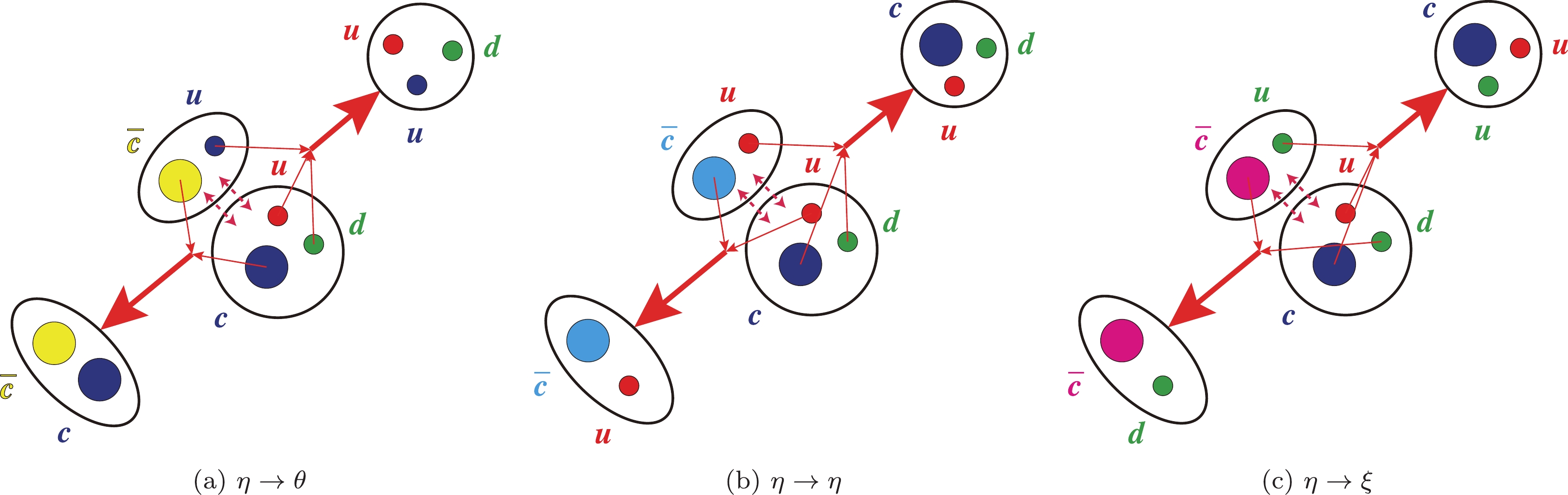
Figure 5. (color online) Fall-apart decays of the
$\bar D^{(*)0} \Sigma_c^{(*)+}$ molecular states investigated using the η currents. There are three possible decay processes: a)$\eta \rightarrow \theta$ , b)$\eta \rightarrow \eta$ , and c)$\eta \rightarrow \xi$ . Their probabilities are the same (33%) if only considering the color degree of freedom. Taken from Ref. [76].$ \begin{aligned}[b] &\;\; \left[\delta^{ab} \bar c_a u_b\right] \; \left[\epsilon^{cde} u_c d_d c_e\right] \\ \underline{\underline {{\rm{color}}}} &\;\; {1\over3}\delta^{ae} \epsilon^{bcd} \; \bar c_au_b \; u_c d_d c_e + \cdots \\ \underline{\underline {{\rm{Fierz}}}} &\;\; {1\over3} \; \left[\delta^{ae}\bar c_a c_e\right] \; \left[\epsilon^{bcd} u_c d_d u_b\right] + \cdots . \end{aligned} $

(110) In particular, we must apply Fierz rearrangement in the first and third steps to interchange both the color and Dirac indices of the
$ u_b $ and$ c_e $ quark fields.The above decay process can be described by the Fierz rearrangement given in Eq. (92), from which we extract the following two decay channels that are kinematically allowed:
1. The decay of
$ |\bar D^0 \Sigma_c^{*+}; 3/2^- \rangle $ into$ \eta_c p $ is contributed by$ [\bar c_a \gamma_\mu \gamma_5 c_a]N $ .$ \begin{aligned}[b] & \langle \bar D^0 \Sigma_c^{*+}; 3/2^-(q) \; |\; \eta_c(q_1)\; p(q_2) \rangle \\ \approx& {a_4}\; {\rm i} f_{\eta_c} f_p q_1^\mu \; \bar u^\alpha \left( - {1\over32} g_{\alpha\mu} \gamma_5 - {{\rm i}\over96} \sigma_{\alpha\mu} \gamma_5 \right) u_p \, , \end{aligned} $

(111) where
$ u_\alpha $ and$ u_p $ are spinors of$ |\bar D^0 \Sigma_c^{*+}; 3/2^- \rangle $ and the proton, respectively.$ a_4 $ is an overall factor related to the coupling of$ \eta_4 $ to$ |\bar D^0 \Sigma_c^{*+}; 3/2^- \rangle $ and the dynamical process of Fig. 5(a).2. The decay of
$ |\bar D^0 \Sigma_c^{*+}; 3/2^- \rangle $ into$ J/\psi p $ is contributed by both$ [\bar c_a \gamma_\mu c_a]N $ and$ [\bar c_a \sigma_{\mu\nu} c_a]N $ .$ \begin{aligned}[b] & \langle \bar D^0 \Sigma_c^{*+}; 3/2^-(q) | J/\psi(q_1,\epsilon_1)\; p(q_2) \rangle \\ \approx& {a_4}\; m_{J/\psi} f_{J/\psi} f_p \epsilon_1^\mu \; \bar u^\alpha \left( - {1\over32} g_{\alpha\mu} - {{\rm i}\over96} \sigma_{\alpha\mu} \right) u_p \\ &+ {a_4}\; {\rm i}f^T_{J/\psi} f_p \; \left(q_1^\mu \epsilon_1^\nu - q_1^\nu \epsilon_1^\mu \right) \\ &\times \bar u^\alpha \left( {{\rm i}\over48} g_{\alpha\mu}\gamma_\nu + {1\over96} \epsilon_{\alpha\mu\nu\rho} \gamma^\rho \gamma_5 \right) u_p \, . \end{aligned} $

(112) Subsequently, we study Eq. (102). As depicted in Fig. 5(b), when the
$ \bar c_a $ and$ u_c $ quarks meet and the other three quarks meet simultaneously,$ |\bar D^0 \Sigma_c^{*+}; 3/2^- \rangle $ can decay into one charmed meson and one charmed baryon. Similarly, we can study the decay process depicted in Fig. 5(c). These two processes can be described by the Fierz rearrangement given in Eq. (102), from which we extract only one decay channel that is kinematically allowed:$ 3. $ The decay of$ |\bar D^0 \Sigma_c^{*+}; 3/2^- \rangle $ into$ \bar D^{*0} \Lambda_c^+ $ is contributed by$ [\bar c_a \gamma_\mu u_a]\Lambda_c^+ $ :$ \begin{aligned}[b] & \langle \bar D^0 \Sigma_c^{*+}; 3/2^-(q) \; |\; \bar D^{*0}(q_1,\epsilon_1)\; \Lambda_c^+(q_2) \rangle \\ \approx& {b_4}\; m_{D^*} f_{D^*} f_{\Lambda_c} \epsilon_1^\mu \; \bar u^\alpha \left( {1\over16}g_{\alpha\mu} + {{\rm i}\over48}\sigma_{\alpha\mu} \right) u_{\Lambda_c} \, , \end{aligned} $

(113) where
$ u_{\Lambda_c} $ is the Dirac spinor of$ \Lambda_c^+ $ .$ b_4 $ is an overall factor related to the coupling of$ \eta_4 $ to$ |\bar D^0 \Sigma_c^{*+}; 3/2^- \rangle $ and the dynamical processes of Fig. 5(b, c).Assuming the mass of
$ |\bar D^0 \Sigma_c^{*+}; 3/2^- \rangle $ to be approximately$ M_{D} + M_{\Sigma_c^*} \approx 4385 $ MeV, we summarize the above decay amplitudes to obtain the following partial decay widths:$ \begin{aligned}[b] \Gamma(|\bar D^0 \Sigma_c^{*+}; 3/2^- \rangle \to \eta_c p ) =& a_4^2 \; 42 \; {\rm{GeV}}^7 \, , \\ \Gamma(|\bar D^0 \Sigma_c^{*+}; 3/2^- \rangle \to J/\psi p ) =& a_4^2 \; 60 \; {\rm{GeV}}^7 \, , \\ \Gamma(|\bar D^0 \Sigma_c^{*+}; 3/2^- \rangle \to \bar D^{*0} \Lambda_c^+ ) =& b_4^2 \; 1.5 \times 10^{4}\; {\rm{GeV}}^7 \, . \end{aligned} $

(114) There are two different terms,
$ A \equiv [\bar c_a \gamma_\mu c_a]N $ and$ B \equiv [\bar c_a \sigma_{\mu\nu} c_a]N $ , both of which can contribute to the decay of$ |\bar D^0 \Sigma_c^{*+}; 3/2^- \rangle $ into$ J/\psi p $ . Their individual contributions are$ \begin{aligned}[b] \Gamma(|\bar D^0 \Sigma_c^{*+}; 3/2^- \rangle \to J/\psi p )\big|_A =& a_4^2 \; 1.0 \times 10^{4}\; {\rm{GeV}}^7 \, , \\ \Gamma(|\bar D^0 \Sigma_c^{*+}; 3/2^- \rangle \to J/\psi p )\big|_B =& a_4^2 \; 1.1 \times 10^{4}\; {\rm{GeV}}^7 \, . \end{aligned} $

(115) Hence, their contributions are at the same level but almost cancel each other out, suggesting that their interference is important. However, the phase angle between them, that is, the phase angle between the two coupling constants
$ f_{J/\psi} $ and$ f_{J/\psi}^T $ , cannot be well determined in the present study. We investigate its relevant (theoretical) uncertainty in Appendix B. -
To study
$ |D^{-} \Sigma_c^{*++}; 3/2^- \rangle $ , we use the$ \xi_4 $ current and Fierz rearrangements given in Eqs. (96) and (106). Assuming its mass to be the same as that of$ |\bar D^{0} \Sigma_c^{*+}; 3/2^- \rangle $ , we obtain the following partial decay widths:$ \begin{aligned}[b] \Gamma(|D^- \Sigma_c^{*++}; 3/2^- \rangle \to \eta_c p ) =& a_4^2 \; 84 \; {\rm{GeV}}^7 \, , \\ \Gamma(|D^- \Sigma_c^{*++}; 3/2^- \rangle \to J/\psi p ) =& a_4^2 \; 120 \; {\rm{GeV}}^7 \, , \\ \Gamma(|D^- \Sigma_c^{*++}; 3/2^- \rangle \to \bar D^{*0} \Lambda_c^+ ) =& b_4^2 \; 3.0 \times 10^{4}\; {\rm{GeV}}^7 \, . \end{aligned} $

(116) Here, we use the same overall factors
$ a_4 $ and$ b_4 $ as those for the$ \eta_4 $ current. -
To study
$ |\bar D^{*0} \Sigma_c^{*+}; 1/2^- \rangle $ , we use the$ \eta_5 $ current and Fierz rearrangements given in Eqs. (93) and (103). Assuming its mass to be approximately$ M_{D^*} + M_{\Sigma_c^*} \approx 4527 $ MeV, we obtain the following partial decay widths:$ \begin{aligned}[b] \Gamma(|\bar D^{*0} \Sigma_c^{*+}; 1/2^- \rangle \to \eta_c p ) =& a_5^2 \; 3.3 \times 10^{5} \; {\rm{GeV}}^7 \, , \\ \Gamma(|\bar D^{*0} \Sigma_c^{*+}; 1/2^- \rangle \to J/\psi p ) =& a_5^2 \; 1.0 \times 10^{4} \; {\rm{GeV}}^7 \, , \\ \Gamma(|\bar D^{*0} \Sigma_c^{*+}; 1/2^- \rangle \to \chi_{c0} p ) =& a_5^2 \; 3.2 \times 10^{3} \; {\rm{GeV}}^7 \, , \\ \Gamma(|\bar D^{*0} \Sigma_c^{*+}; 1/2^- \rangle \to \chi_{c1} p ) =& a_5^2 \; 1.1 \times 10^{3} \; {\rm{GeV}}^7 \, , \\ \Gamma(|\bar D^{*0} \Sigma_c^{*+}; 1/2^- \rangle \to h_{c} p ) =& a_5^2 \; 220 \; {\rm{GeV}}^7 \, , \\ \Gamma(|\bar D^{*0} \Sigma_c^{*+}; 1/2^- \rangle \to \bar D^{0} \Lambda_c^+ ) =& b_5^2 \; 3.5 \times 10^{5}\; {\rm{GeV}}^7 \, , \\ \Gamma(|\bar D^{*0} \Sigma_c^{*+}; 1/2^- \rangle \to \bar D^{*0} \Lambda_c^+ ) =& b_5^2 \; 1.6 \times 10^{4}\; {\rm{GeV}}^7 \, , \\ \Gamma(|\bar D^{*0} \Sigma_c^{*+}; 1/2^- \rangle \to \bar D^{0} \Sigma_c^+ )=& b_5^2 \; 1.4 \times 10^{4}\; {\rm{GeV}}^7 \, , \\ \Gamma(|\bar D^{*0} \Sigma_c^{*+}; 1/2^- \rangle \to D^- \Sigma_c^{++} ) =& b_5^2 \; 2.9 \times 10^{4}\; {\rm{GeV}}^7 \, , \\ \Gamma(|\bar D^{*0} \Sigma_c^{*+}; 1/2^- \rangle \to \bar D^{*0} \Sigma_c^+ ) =& b_5^2 \; 3.3 \times 10^{4}\; {\rm{GeV}}^7 \, , \\ \Gamma(|\bar D^{*0} \Sigma_c^{*+}; 1/2^- \rangle \to D^{*-} \Sigma_c^{++} ) =& b_5^2 \; 6.6 \times 10^{4}\; {\rm{GeV}}^7 \, , \end{aligned} $

(117) where
$ a_5 $ and$ b_5 $ are two overall factors. -
To study
$ |D^{*-} \Sigma_c^{*++}; 1/2^- \rangle $ , we use the$ \xi_5 $ current and the Fierz rearrangements given in Eqs. (97) and (107). Assuming its mass to be the same as that of$ |\bar D^{*0} \Sigma_c^{*+}; 1/2^- \rangle $ , we obtain the following partial decay widths:$ \begin{aligned}[b] \Gamma(|D^{*-} \Sigma_c^{*++}; 1/2^- \rangle \to \eta_c p ) =& a_5^2 \; 6.5 \times 10^{5} \; {\rm{GeV}}^7 \, , \\ \Gamma(|D^{*-} \Sigma_c^{*++}; 1/2^- \rangle \to J/\psi p ) =& a_5^2 \; 2.1 \times 10^{4} \; {\rm{GeV}}^7 \, , \\ \Gamma(|D^{*-} \Sigma_c^{*++}; 1/2^- \rangle \to \chi_{c0} p ) =& a_5^2 \; 6.4 \times 10^{3} \; {\rm{GeV}}^7 \, , \\ \Gamma(|D^{*-} \Sigma_c^{*++}; 1/2^- \rangle \to \chi_{c1} p ) =& a_5^2 \; 2.1 \times 10^{3} \; {\rm{GeV}}^7 \, , \\ \Gamma(|D^{*-} \Sigma_c^{*++}; 1/2^- \rangle \to h_{c} p ) =& a_5^2 \; 450 \; {\rm{GeV}}^7 \, , \\ \Gamma(|D^{*-} \Sigma_c^{*++}; 1/2^- \rangle \to \bar D^{0} \Lambda_c^+ ) =& b_5^2 \; 7.0 \times 10^{5}\; {\rm{GeV}}^7 \, , \\ \Gamma(|D^{*-} \Sigma_c^{*++}; 1/2^- \rangle \to \bar D^{*0} \Lambda_c^+ ) =& b_5^2 \; 3.1 \times 10^{4}\; {\rm{GeV}}^7 \, , \\ \Gamma(|D^{*-} \Sigma_c^{*++}; 1/2^- \rangle \to \bar D^{0} \Sigma_c^+ ) =& b_5^2 \; 2.9 \times 10^{4}\; {\rm{GeV}}^7 \, , \\ \Gamma(|D^{*-} \Sigma_c^{*++}; 1/2^- \rangle \to \bar D^{*0} \Sigma_c^+ ) =& b_5^2 \; 6.6 \times 10^{4}\; {\rm{GeV}}^7 \, . \end{aligned} $

(118) -
To study
$ |\bar D^{*0} \Sigma_c^{*+}; 3/2^- \rangle $ , we use the$ \eta_6 $ current and Fierz rearrangements given in Eqs. (94) and (104). Assuming its mass to be the same as that of$ |\bar D^{*0} \Sigma_c^{*+}; 1/2^- \rangle $ , we obtain the following partial decay widths:$ \begin{aligned}[b] \Gamma(|\bar D^{*0} \Sigma_c^{*+}; 3/2^- \rangle \to \eta_c p ) =& a_6^2 \; 750 \; {\rm{GeV}}^7 \, , \\ \Gamma(|\bar D^{*0} \Sigma_c^{*+}; 3/2^- \rangle \to J/\psi p ) =& a_6^2 \; 1.2 \times 10^{5} \; {\rm{GeV}}^7 \, , \\ \Gamma(|\bar D^{*0} \Sigma_c^{*+}; 3/2^- \rangle \to \chi_{c0} p ) =& a_6^2 \; 960 \; {\rm{GeV}}^7 \, ,\\ \Gamma(|\bar D^{*0} \Sigma_c^{*+}; 3/2^- \rangle \to \bar D^{*0} \Lambda_c^+ )=& b_6^2 \; 4.5 \times 10^{4}\; {\rm{GeV}}^7 \, , \\ \end{aligned} $

$ \begin{aligned}[b] \Gamma(|\bar D^{*0} \Sigma_c^{*+}; 3/2^- \rangle \to \bar D^{0} \Sigma_c^+ ) =& b_6^2 \; 36\; {\rm{GeV}}^7 \, , \\ \Gamma(|\bar D^{*0} \Sigma_c^{*+}; 3/2^- \rangle \to D^- \Sigma_c^{++} ) =& b_6^2 \; 71\; {\rm{GeV}}^7 \, , \\ \Gamma(|\bar D^{*0} \Sigma_c^{*+}; 3/2^- \rangle \to \bar D^{*0} \Sigma_c^+ ) =& b_6^2 \; 4.3 \times 10^{4}\; {\rm{GeV}}^7 \, , \\ \Gamma(|\bar D^{*0} \Sigma_c^{*+}; 3/2^- \rangle \to D^{*-} \Sigma_c^{++} ) =& b_6^2 \; 8.7 \times 10^{4}\; {\rm{GeV}}^7 \, , \end{aligned} $

(119) where
$ a_6 $ and$ b_6 $ are two overall factors. -
To study
$ |D^{*-} \Sigma_c^{*++}; 3/2^- \rangle $ , we use the$ \xi_6 $ current and Fierz rearrangements given in Eqs. (98) and (108). Assuming its mass to be the same as that of$ |\bar D^{*0} \Sigma_c^{*+}; 1/2^- \rangle $ , we obtain the following partial decay widths:$ \begin{aligned}[b] \Gamma(|D^{*-} \Sigma_c^{*++}; 3/2^- \rangle \to \eta_c p ) =& a_6^2 \; 1.5 \times 10^{3} \; {\rm{GeV}}^7 \, , \\ \Gamma(|D^{*-} \Sigma_c^{*++}; 3/2^- \rangle \to J/\psi p ) =& a_6^2 \; 2.3 \times 10^{5} \; {\rm{GeV}}^7 \, , \\ \Gamma(|D^{*-} \Sigma_c^{*++}; 3/2^- \rangle \to \chi_{c0} p ) =& a_6^2 \; 1.9 \times 10^{3} \; {\rm{GeV}}^7 \, , \\ \Gamma(|D^{*-} \Sigma_c^{*++}; 3/2^- \rangle \to \bar D^{*0} \Lambda_c^+ ) =& b_6^2 \; 9.1 \times 10^{4}\; {\rm{GeV}}^7 \, , \\ \Gamma(|D^{*-} \Sigma_c^{*++}; 3/2^- \rangle \to \bar D^{0} \Sigma_c^+ ) =& b_6^2 \; 71\; {\rm{GeV}}^7 \, , \\ \Gamma(|D^{*-} \Sigma_c^{*++}; 3/2^- \rangle \to \bar D^{*0} \Sigma_c^+ ) =& b_6^2 \; 8.7 \times 10^{4}\; {\rm{GeV}}^7 \, . \end{aligned} $

(120) -
To study
$ |\bar D^{*0} \Sigma_c^{*+}; 5/2^- \rangle $ , we use the$ \eta_7 $ current and Fierz rearrangements given in Eqs. (95) and (105); however, we do not obtain any non-zero decay channels. This state probably mainly decays into spin-1 mesons and spin-3/2 baryons, such as$ J/\psi N^* $ and$ D^* \Sigma_c^* $ . However, these final states are not investigated in the present study. The same results are obtained for$ |D^{*-} \Sigma_c^{*++}; 5/2^- \rangle $ . -
In this subsection, we collect the results calculated in the previous subsection to further study the decay properties of the
$ \bar D^{(*)} \Sigma_c^* $ molecular states with$ I=1/2 $ .Combining the results of Sec. V.C.1 and Sec. V.C.2, we obtain the following partial decay widths for
$ |\bar D \Sigma_c^{*}; 3/2^- \rangle $ of$ I=1/2 $ :$ \begin{aligned}[b] \Gamma(|\bar D \Sigma_c^{*}; 3/2^- \rangle \to \eta_c p ) =& a_4^2 \; 130 \; {\rm{GeV}}^7 \, , \\ \Gamma(|\bar D \Sigma_c^{*}; 3/2^- \rangle \to J/\psi p ) =& a_4^2 \; 180 \; {\rm{GeV}}^7 \, , \\ \Gamma(|\bar D \Sigma_c^{*}; 3/2^- \rangle \to \bar D^{*0} \Lambda_c^+ ) =& b_4^2 \; 4.5 \times 10^{4}\; {\rm{GeV}}^7 \, . \end{aligned} $

(121) Combining the results of Sec. V.C.3 and Sec. V.C.4, we obtain the following partial decay widths for
$ |\bar D^* \Sigma_c^{*}; 1/2^- \rangle $ of$ I=1/2 $ :$ \begin{aligned}[b] \Gamma(|\bar D^{*} \Sigma_c^{*}; 1/2^- \rangle \to \eta_c p ) =a_5^2 \; 9.8 \times 10^{5} \; {\rm{GeV}}^7 \, , \end{aligned} $

$ \begin{aligned}[b] \Gamma(|\bar D^{*} \Sigma_c^{*}; 1/2^- \rangle \to J/\psi p ) =& a_5^2 \; 3.1 \times 10^{4} \; {\rm{GeV}}^7 \, , \\ \Gamma(|\bar D^{*} \Sigma_c^{*}; 1/2^- \rangle \to \chi_{c0} p ) =& a_5^2 \; 9.5 \times 10^{3} \; {\rm{GeV}}^7 \, , \\ \Gamma(|\bar D^{*} \Sigma_c^{*}; 1/2^- \rangle \to \chi_{c1} p ) =& a_5^2 \; 3.2 \times 10^{3} \; {\rm{GeV}}^7 \, , \\ \Gamma(|\bar D^{*} \Sigma_c^{*}; 1/2^- \rangle \to h_{c} p ) =& a_5^2 \; 670 \; {\rm{GeV}}^7 \, , \\ \Gamma(|\bar D^{*} \Sigma_c^{*}; 1/2^- \rangle \to \bar D^{0} \Lambda_c^+ ) =& b_5^2 \; 1.1 \times 10^{6}\; {\rm{GeV}}^7 \, , \\ \Gamma(|\bar D^{*} \Sigma_c^{*}; 1/2^- \rangle \to \bar D^{*0} \Lambda_c^+ ) =& b_5^2 \; 4.7 \times 10^{4}\; {\rm{GeV}}^7 \, , \\ \Gamma(|\bar D^{*} \Sigma_c^{*}; 1/2^- \rangle \to \bar D^{0} \Sigma_c^+ ) =& b_5^2 \; 4.8 \times 10^{3}\; {\rm{GeV}}^7 \, , \\ \Gamma(|\bar D^{*} \Sigma_c^{*}; 1/2^- \rangle \to D^- \Sigma_c^{++} ) =& b_5^2 \; 9.6 \times 10^{3}\; {\rm{GeV}}^7 \, , \\ \Gamma(|\bar D^{*} \Sigma_c^{*}; 1/2^- \rangle \to \bar D^{*0} \Sigma_c^+ ) =& b_5^2 \; 1.1 \times 10^{4}\; {\rm{GeV}}^7 \, , \\ \Gamma(|\bar D^{*} \Sigma_c^{*}; 1/2^- \rangle \to D^{*-} \Sigma_c^{++} ) =& b_5^2 \; 2.2 \times 10^{4}\; {\rm{GeV}}^7 \, . \end{aligned} $

(122) Combining the results of Sec. V.C.5 and Sec. V.C.6, we obtain the following partial decay widths for
$ |\bar D^* \Sigma_c^{*}; 3/2^- \rangle $ of$ I=1/2 $ :$ \begin{aligned}[b] \Gamma(|\bar D^{*} \Sigma_c^{*}; 3/2^- \rangle \to \eta_c p ) =& a_6^2 \; 2.2 \times 10^{3} \; {\rm{GeV}}^7 \, , \\ \Gamma(|\bar D^{*} \Sigma_c^{*}; 3/2^- \rangle \to J/\psi p ) =& a_6^2 \; 3.5 \times 10^{5} \; {\rm{GeV}}^7 \, , \\ \Gamma(|\bar D^{*} \Sigma_c^{*}; 3/2^- \rangle \to \chi_{c0} p ) =& a_6^2 \; 2.9 \times 10^{3} \; {\rm{GeV}}^7 \, , \\ \Gamma(|\bar D^{*} \Sigma_c^{*}; 3/2^- \rangle \to \bar D^{*0} \Lambda_c^+ ) =& b_6^2 \; 1.4 \times 10^{5}\; {\rm{GeV}}^7 \, , \\ \Gamma(|\bar D^{*} \Sigma_c^{*}; 3/2^- \rangle \to \bar D^{0} \Sigma_c^+ ) =& b_6^2 \; 12\; {\rm{GeV}}^7 \, , \\ \Gamma(|\bar D^{*} \Sigma_c^{*}; 3/2^- \rangle \to D^- \Sigma_c^{++} ) =& b_6^2 \; 24\; {\rm{GeV}}^7 \, , \\ \Gamma(|\bar D^{*} \Sigma_c^{*}; 3/2^- \rangle \to \bar D^{*0} \Sigma_c^+ ) =& b_6^2 \; 1.4 \times 10^{4}\; {\rm{GeV}}^7 \, , \\ \Gamma(|\bar D^{*} \Sigma_c^{*}; 3/2^- \rangle \to D^{*-} \Sigma_c^{++} ) =& b_6^2 \; 2.9 \times 10^{4}\; {\rm{GeV}}^7 \, . \end{aligned} $

(123) We do not obtain any non-zero decay channels for
$ |\bar D^* \Sigma_c^{*}; 5/2^- \rangle $ of$ I=1/2 $ . This state probably mainly decays into spin-1 mesons and spin-3/2 baryons, such as$ J/\psi N^* $ and$ \bar D^* \Sigma_c^* $ . However, these final states are not investigated in the present study.The decay properties of the
$ \bar D^{(*)} \Sigma_c $ molecular states havebeen investigated in Ref. [76], including$ |\bar D \Sigma_c; 1/2^- \rangle $ ,$ |\bar D^{*} \Sigma_c; 1/2^- \rangle $ , and$ |\bar D^{*} \Sigma_c; 3/2^- \rangle $ . There, we used them to explain$ P_c(4312)^+ $ ,$ P_c(4440)^+ $ , and$ P_c(4457)^+ $ , respectively. However, we find that$ P_c(4440)^+ $ and$ P_c(4457)^+ $ can be better interpreted in our framework as$ |\bar D^{*} \Sigma_c; 3/2^- \rangle $ and$ |\bar D^{*} \Sigma_c; 1/2^- \rangle $ , respectively/inversely.Accordingly, we assume the masses of
$ |\bar D \Sigma_c; 1/2^- \rangle $ ,$ |\bar D^{*} \Sigma_c; 1/2^- \rangle $ , and$ |\bar D^{*} \Sigma_c; 3/2^- \rangle $ to be$ M_{P_c(4312)^+} = 4311.9 $ MeV,$ M_{P_c(4457)^+} = 4457.3 $ MeV, and$ M_{P_c(4440)^+} = 4440.3 $ MeV, respectively. Recalculations are performed, and we summarize the results here. Note that a) some errors were detected in the results of Ref. [76] when calculating$ \Gamma(|\bar D^* \Sigma_c; 1/2^- \rangle \to J/\psi p) $ , and b) different notations are used here for the overall factors.For
$ |\bar D \Sigma_c; 1/2^- \rangle $ of$ I=1/2 $ , we find$ \begin{aligned}[b] \Gamma(|\bar D \Sigma_c; 1/2^- \rangle \to \eta_c p ) =a_1^2 \; 3.2 \times 10^{5}\; {\rm{GeV}}^7 \, , \end{aligned} $

$ \begin{aligned}[b] \Gamma(|\bar D \Sigma_c; 1/2^- \rangle \to J/\psi p ) =& a_1^2 \; 8.5 \times 10^{4}\; {\rm{GeV}}^7 \, , \\ \Gamma(|\bar D \Sigma_c; 1/2^- \rangle \to \bar D^{*0} \Lambda_c^+ ) =& b_1^2 \; 5.9 \times 10^{4}\; {\rm{GeV}}^7 \, . \end{aligned} $

(124) For
$ |\bar D^{*} \Sigma_c; 1/2^- \rangle $ of$ I=1/2 $ , we find$ \begin{aligned}[b] \Gamma(|\bar D^{*} \Sigma_c; 1/2^- \rangle \to \eta_c p ) =& a_2^2 \; 1.8 \times 10^{5}\; {\rm{GeV}}^7 \, , \\ \Gamma(|\bar D^{*} \Sigma_c; 1/2^- \rangle \to J/\psi p ) =& a_2^2 \; 5.1 \times 10^{5}\; {\rm{GeV}}^7 \, , \\ \Gamma(|\bar D^{*} \Sigma_c; 1/2^- \rangle \to \chi_{c0} p ) =& a_2^2 \; 8.0 \times 10^{3}\; {\rm{GeV}}^7 \, , \\ \Gamma(|\bar D^{*} \Sigma_c; 1/2^- \rangle \to \chi_{c1} p ) =& a_2^2 \; 200\; {\rm{GeV}}^7 \, , \\ \Gamma(|\bar D^{*} \Sigma_c; 1/2^- \rangle \to \bar D^{0} \Lambda_c^+ ) =& b_2^2 \; 1.7 \times 10^{6}\; {\rm{GeV}}^7 \, , \\ \Gamma(|\bar D^{*} \Sigma_c; 1/2^- \rangle \to \bar D^{*0} \Lambda_c^+ ) =& b_2^2 \; 6.0 \times 10^{5}\; {\rm{GeV}}^7 \, , \\ \Gamma(|\bar D^{*} \Sigma_c; 1/2^- \rangle \to \bar D^{0} \Sigma_c^+ ) =& b_2^2 \; 5.9 \times 10^{4}\; {\rm{GeV}}^7 \, , \\ \Gamma(|\bar D^{*} \Sigma_c; 1/2^- \rangle \to D^- \Sigma_c^{++} ) =& b_2^2 \; 1.2 \times 10^{5}\; {\rm{GeV}}^7 \, . \end{aligned} $

(125) For
$ |\bar D^{*} \Sigma_c; 3/2^- \rangle $ of$ I=1/2 $ , we find$ \begin{aligned}[b] \Gamma(|\bar D^{*} \Sigma_c; 3/2^- \rangle \to \eta_c p ) =& a_3^2 \; 670\; {\rm{GeV}}^7 \, , \\ \Gamma(|\bar D^{*} \Sigma_c; 3/2^- \rangle \to J/\psi p ) =& a_3^2 \; 1.4 \times 10^{5}\; {\rm{GeV}}^7 \, , \\ \Gamma(|\bar D^{*} \Sigma_c; 3/2^- \rangle \to \bar D^{*0} \Lambda_c^+ ) =& b_3^2 \; 4.6 \times 10^{4}\; {\rm{GeV}}^7 \, , \\ \Gamma(|\bar D^{*} \Sigma_c; 3/2^- \rangle \to \bar D^{0} \Sigma_c^+ ) =& b_3^2 \; 1.4 \; {\rm{GeV}}^7 \, , \\ \Gamma(|\bar D^{*} \Sigma_c; 3/2^- \rangle \to D^- \Sigma_c^{++} ) =& b_3^2 \; 2.7 \; {\rm{GeV}}^7 \, . \end{aligned} $

(126) We use the above partial decay widths to further derive their corresponding relative branching ratios. The obtained results are summarized in Table 3, where a new parameter
$ t \equiv {b_i^2 / a_i^2} $ ($ i=1\cdots7 $ ) is introduced to measure which processes occur more easily, the process depicted in Fig. 5(a) or the processes depicted in Fig. 5(b, c). We discuss these results in Sec. VI.Configuration Decay channels Productions $J/\psi p$ 

$\eta_c p$ 

$\chi_{c0} p$ 

$\chi_{c1} p$ 

$h_c p$ 

$\bar D^{0} \Lambda_c^+$ 

$\bar D^{*0} \Lambda_c^+$ 

$\bar D^{0} \Sigma_c^+$ 

$D^{-} \Sigma_c^{++}$ 

$\bar D^{*0} \Sigma_c^+$ 

$D^{*-} \Sigma_c^{++}$ 

${\cal{R}}_1$ 

${\cal{R}}_2$ 

$|\bar D \Sigma_c; 1/2^- \rangle$ 

$1$ 

$3.8$ 

− − − − $0.69t$ 

− − − − $8.2$ 

$2.0$ 

$|\bar D^{*} \Sigma_c; 1/2^- \rangle$ 

$1$ 

$0.35$ 

$0.016$ 

$10^{-4}$ 

− $3.4t$ 

$1.2t$ 

$0.12t$ 

$0.23t$ 

− − $1.2$ 

$0.25$ 

$|\bar D^{*} \Sigma_c; 3/2^- \rangle$ 

$1$ 

$0.005$ 

− − − − $0.34t$ 

$10^{-5}t$ 

$10^{-5}t$ 

− − $\bf1$ 

$\bf1$ 

$|\bar D \Sigma_c^*; 3/2^- \rangle$ 

$1$ 

$0.70$ 

− − − − $250t$ 

− − − − − − $|\bar D^* \Sigma_c^*; 1/2^- \rangle$ 

$1$ 

$31$ 

$0.30$ 

$0.10$ 

$0.02$ 

$34t$ 

$1.5t$ 

$0.15t$ 

$0.30t$ 

$0.35t$ 

$0.70t$ 

$4.8$ 

$0.09$ 

$|\bar D^* \Sigma_c^*; 3/2^- \rangle$ 

$1$ 

$0.006$ 

− $0.008$ 

− − $0.39t$ 

$10^{-5}t$ 

$10^{-4}t$ 

$0.04t$ 

$0.08t$ 

$0.18$ 

$0.16$ 

$|\bar D^* \Sigma_c^*; 5/2^- \rangle$ 

− − − − Table 3. Relative branching ratios of the
$ \bar D^{(*)} \Sigma_c^{(*)} $ hadronic molecular states and their relative production rates in$ \Lambda_b^0 $ decays. In the 2rd-12th columns, we show the branching ratios relative to the$ J/\psi p $ channel, such as$ {{\cal{B}}(P_c \to \eta_c p)\over{\cal{B}}(P_c \to J/\psi p)} $ in the 3rd column. The parameter$ t \equiv {b_i^2 / a_i^2} $ ($ i=1\cdots7 $ ) is introduced to measure which processes occur more easily, the process depicted in Fig. 5(a) or the processes depicted in Fig. 5(b, c). In the 13th column, we show the ratio$ {\cal{R}}_1(P_c) \equiv {{\cal{B}}\left(\Lambda_b^0 \rightarrow P_c K^- \right) \over {\cal{B}}\left(\Lambda_b^0 \rightarrow |\bar D^* \Sigma_c \rangle_{3/2^-} K^- \right)} $ , and in the 14th column, we show the ratio$ {\cal{R}}_2(P_c) \equiv { {\cal{B}}(\Lambda_b^0 \to P_c K^- \to J/\psi p K^-) \over {\cal{B}}(\Lambda_b^0 \to |\bar D^* \Sigma_c \rangle_{3/2^-} K^- \to J/\psi p K^-) } $ . To calculate$ {\cal{R}}_2 $ , we a) simply assume$ t=1 $ and b) neglect all the spin-3/2 baryons that$ P_c $ can decay into, such as the$ J/\psi N^* $ and$ \bar D \Sigma_c^* $ final states. -
In this paper, we systematically investigate the seven possible
$ \bar D^{(*)} \Sigma_c^{(*)} $ hadronic molecular states of$ I=1/2 $ , including$ \bar D \Sigma_c $ of$ J^P = {1/2}^- $ ,$ \bar D^* \Sigma_c $ of$ J^P = {(1/2)}^-/ {(3/2)}^- $ ,$ \bar D \Sigma_c^* $ of$ J^P = {3/2}^- $ , and$ \bar D^* \Sigma_c^* $ of$J^P = {(1/2)}^-/ {(3/2)}^-/ {(5/2)}^-$ .First, we systematically construct their corresponding interpolating currents and calculate their masses and decay constants using QCD sum rules. The results are summarized in Table 1, supporting the interpretations of
$ P_c(4312)^+ $ ,$ P_c(4440)^+ $ , and$ P_c(4457)^+ $ [5] as the$ \bar D \Sigma_c $ and$ \bar D^* \Sigma_c $ molecular states. However, the accuracy of our sum rule results is not good enough to distinguish or indentify them. To better understand them, we further study their production and decay properties. The decay constants$ f_X $ extracted using QCD sum rules are important input parameters.Second, we use current algebra to study the production of
$ \bar D^{(*)} \Sigma_c^{(*)} $ molecular states in$ \Lambda_b^0 $ decays. We derive the relative production rates$ {\cal{R}}_1(P_c) \equiv {{\cal{B}}\left(\Lambda_b^0 \rightarrow P_c K^- \right) \over {\cal{B}}\left(\Lambda_b^0 \rightarrow |\bar D^* \Sigma_c \rangle_{3/2^-} K^- \right)} \, , $

(127) and the obtained results are summarized in Table 3.
Third, we use the Fierz rearrangement of the Dirac and color indices to study the decay properties of the
$ \bar D^{(*)} \Sigma_c^{*} $ molecular states, including their decays into charmonium mesons and spin-1/2 light baryons as well as charmed mesons and spin-1/2 charmed baryons, such as$ J/\psi p $ and$ \bar D \Lambda_c $ . We calculate their relative branching ratios, and the obtained results are also summarized in Table 3. The parameter$ t \equiv {b_i^2 / a_i^2} $ ($ i=1\cdots7 $ ) is introduced to measure which processes occur more easily, the process depicted in Fig. 5(a) or the processes depicted in Fig. 5(b, c). Generally, the exchange of one light quark with another light quark may be easier than its exchange with a heavy quark [125]; therefore, it can be the case that$ t \geq 1 $ .In Table 3, we simply assume
$ t=1 $ to further calculate the ratio$ {\cal{R}}_1 $ in the$ J/\psi p $ mass spectrum, that is,$ {\cal{R}}_2(P_c) \equiv { {\cal{B}}(\Lambda_b^0 \to P_c K^- \to J/\psi p K^-) \over {\cal{B}}(\Lambda_b^0 \to |\bar D^* \Sigma_c \rangle_{3/2^-} K^- \to J/\psi p K^-) } \, . $

(128) To calculate this ratio, we neglect all spin-3/2 baryons that
$ P_c $ can decay into, such as the$ J/\psi N^* $ and$ \bar D \Sigma_c^* $ final states.Before drawing conclusions, we would like to note the following:
● When studying the masses and decay constants of the
$ \bar D^{(*)} \Sigma_c^{(*)} $ molecular states using QCD sum rules, we calculate two-point correlation functions at the quark-gluon level as inputs, whereas the masses of charmed mesons and baryons at the hadron level are not used as input parameters. Accordingly, the uncertainty/accuracy is moderate but not sufficient to extract the binding energy. This means that our sum rule results can only suggest but not determine a) whether these$ \bar D^{(*)} \Sigma_c^{(*)} $ molecular states exist, and b) whether they are bound or resonance states. Instead, we must assume their existence. We may then use the extracted decay constants to further study their production and decay properties.● When studying the relative production rates of the
$ \bar D^{(*)} \Sigma_c^{(*)} $ molecular states in$ \Lambda_b^0 $ decays using current algebra, we only investigate the hidden-charm pentaquark currents that can couple to these states through an S-wave, that is,$ J_{1\cdots7} $ defined in Eqs. (26)–(40). There may be other currents coupling to these states through a P-wave, which are not considered in the present study. Accordingly,$ |\bar D \Sigma_c^*; 3/2^- \rangle $ and$ |\bar D^* \Sigma_c^*; 5/2^- \rangle $ may still be produced in$ \Lambda_b^0 $ decays through these "P-wave" currents. Note that their omission produces theoretical uncertainties.● When studying the decay properties of the
$ \bar D^{(*)} \Sigma_c^{*} $ molecular states via Fierz rearrangement, we consider the leading-order fall-apart decays described by color-singlet-color-singlet meson-baryon currents but neglect the$ {\cal{O}}(\alpha_s) $ corrections described by color-octet-color-octet meson-baryon currents; therefore, there may be other possible decay channels. Moreover, we do not consider the light/charmed baryon fields of$ J=3/2 $ ; hence, we cannot study their decays into the$ J/\psi N^* $ and$ \bar D \Sigma_c^* $ final states. However, we keep all light/charmed baryon fields that couple to the ground-state light/charmed baryons of$ J^P=1/2^+ $ ; hence, their decays into these final states are well investigated in this paper.Now, we can discuss our uncertainties. The uncertainty on our QCD sum rule results is moderate, whereas the uncertainties on the relative branching ratios as well as the two ratios
$ {\cal{R}}_1 $ and$ {\cal{R}}_2 $ are significantly larger. In the present study, we work under the naïve factorization scheme; therefore, our uncertainties are significantly larger than those of the well-developed QCD factorization scheme [126–128], whose uncertainty is at the 5% level when investigating conventional (heavy) hadrons [129]. However, in this paper, we only calculate the ratios, which significantly reduces our uncertainties. Accordingly, we approximately estimate the uncertainty on the relative branching ratios to be at the$ X^{+100\%}_{-\; 50\%} $ level. Owing to the omission of the "P-wave" pentaquark currents, the uncertainty on the ratio$ {\cal{R}}_1 $ is approximately estimated to be at the$ X^{+200\%}_{-\; 67\%} $ level. We further estimate the uncertainty on the ratio$ {\cal{R}}_2 $ to be at the$ X^{+300\%}_{-\; 75\%} $ level (or even larger due to the assumption that$ t=1 $ and the omission of the spin-3/2 baryons that$ P_c $ can decay into).Finally, we can draw conclusions using the results summarized in Table 3. The LHCb experiment [5] discovered
$ P_c(4312)^+ $ ,$ P_c(4440)^+ $ , and$ P_c(4457)^+ $ and, at the same time, measured their relative contributions${\cal{R}}\; \equiv \;{\cal{B}}\;(\Lambda^0_b \to P_c^+ K^-)\,{\cal{B}}\,(P_c^+ \to J/\psi p)\,/\,{\cal{B}}\,(\,\Lambda^0_b \to J/\psi p K^-)$ to be$ \begin{aligned}[b] {\cal{R}}(P_c(4312)^+) =& 0.30 \pm 0.07 ^{+0.34}_{-0.09} \% \, , \\ {\cal{R}}(P_c(4440)^+) =& 1.11 \pm 0.33 ^{+0.22}_{-0.10} \% \, , \\ {\cal{R}}(P_c(4457)^+) =& 0.53 \pm 0.16 ^{+0.15}_{-0.13} \% \, , \end{aligned} $

(129) from which we can derive
$ \begin{aligned}[b] {{\cal{R}}(P_c(4312)^+) \over {\cal{R}}(P_c(4440)^+)} =& 0.27^{+0.32}_{-0.14} \, , \\ {{\cal{R}}(P_c(4457)^+) \over {\cal{R}}(P_c(4440)^+)} =& 0.48^{+0.25}_{-0.25} \, . \end{aligned} $

(130) These two values are approximately consistent with our results,
$ \begin{aligned}[b] {\cal{R}}_2(|\bar D \Sigma_c; 1/2^- \rangle) =& {{\cal{R}}_2(|\bar D \Sigma_c; 1/2^- \rangle) \over {\cal{R}}_2(|\bar D^* \Sigma_c; 3/2^- \rangle)} \approx 2.0 \, , \\ {\cal{R}}_2(|\bar D^* \Sigma_c; 1/2^- \rangle) =& {{\cal{R}}_2(|\bar D^* \Sigma_c; 1/2^- \rangle) \over {\cal{R}}_2(|\bar D^* \Sigma_c; 3/2^- \rangle)} \approx 0.25 \, , \end{aligned} $

(131) given that their uncertainties are approximately at the
$ X^{+300\%}_{-\; 75\%} $ level.Therefore, our results support the interpretations of
$ P_c(4312)^+ $ ,$ P_c(4440)^+ $ , and$ P_c(4457)^+ $ as$ \bar D \Sigma_c $ of$ J^P = {1/2}^- $ ,$ \bar D^* \Sigma_c $ of$ J^P = {3/2}^- $ , and$ \bar D^* \Sigma_c $ of$ J^P = {1/2}^- $ , respectively. For completeness, we also investigate the interpretations of$ P_c(4440)^+ $ and$ P_c(4457)^+ $ as the$ \bar D^* \Sigma_c $ molecular states of$ J^P = {1/2}^- $ and$ {3/2}^- $ , respectively, and the results are given in Appendix C.Our results suggest that the
$ \bar D^* \Sigma_c^* $ molecular states of$ J^P = 1/2^- $ and$ 3/2^- $ may also be observed in the$ J/\psi p $ invariant mass spectrum of$ \Lambda_b^0 \to J/\psi p K^- $ decays, and their relative contributions are estimated to be$ \begin{aligned}[b] { {\cal{B}}(\Lambda_b^0 \to |\bar D^* \Sigma_c^* \rangle_{1/2^-} K^- \to J/\psi p K^-) \over {\cal{B}}(\Lambda^0_b \to J/\psi p K^-) } \approx 0.1{\text{%}} \, , \end{aligned} $

$ \begin{aligned}[b] { {\cal{B}}(\Lambda_b^0 \to |\bar D^* \Sigma_c^* \rangle_{3/2^-} K^- \to J/\psi p K^-) \over {\cal{B}}(\Lambda^0_b \to J/\psi p K^-) } \approx 0.2{\text{%}} \, . \end{aligned} $

(132) Their relative branching ratios to the
$ \eta_c p $ ,$ \chi_{c0} p $ ,$ \chi_{c1} p $ ,$ h_c p $ ,$ \bar D^{0} \Lambda_c^+ $ ,$ \bar D^{*0} \Lambda_c^+ $ ,$ \bar D^{0} \Sigma_c^+ $ ,$ D^{-} \Sigma_c^{++} $ ,$ \bar D^{*0} \Sigma_c^+ $ , and$ D^{*-} \Sigma_c^{++} $ final states are also given for future experimental searches. -
In this appendix, we list the spectral densities
$ \rho_{1\cdots7}(s) $ extracted for the currents$ J_{1\cdots7} $ . In the following expressions,$ {\cal{F}}(s)=\left[(\alpha+\beta) m_{c}^{2}-\alpha \beta s\right], {\cal{H}}(s)=\left[m_{c}^{2}-\alpha(1-\alpha) s\right]$ , and the integration limits are$ \alpha_{\rm min}={(1-\sqrt{1-4m_c^2/s})}/{2} $ ,$ \alpha_{\rm max}={(1+\sqrt{1-4m_c^2/s})}/{2} $ ,$ \beta_{\rm min}={(\alpha m_c^2)}/{(\alpha s-m_c^2)} $ , and$ \beta_{\rm max}=1-\alpha $ .The spectral density
$ \rho_{1}(s) $ extracted for the current$ J_{1} $ is$ \begin{aligned}[b]\\[-6pt] \rho_{1}(s) =& m_c \left( \rho^{\rm pert}_{1a}(s) + \rho^{{\langle\bar qq\rangle}}_{1a}(s) + \rho^{{\langle GG\rangle}}_{1a}(s)+ \rho^{{\langle\bar qGq\rangle}}_{1a}(s) + \rho^{{\langle\bar qq\rangle}^2}_{1a}(s) + \rho^{{\langle\bar qq\rangle}{\langle\bar qGq\rangle}}_{1a}(s)+ \rho^{{\langle\bar qGq\rangle}^2}_{1a}(s) + \rho^{{\langle\bar qq\rangle}^3}_{1a}(s) \right) \\ &+ \not q \; \; \left( \rho^{\rm pert}_{1b}(s) + \rho^{{\langle\bar qq\rangle}}_{1b}(s) + \rho^{{\langle GG\rangle}}_{1b}(s)+ \rho^{{\langle\bar qGq\rangle}}_{1b}(s) + \rho^{{\langle\bar qq\rangle}^2}_{1b}(s) + \rho^{{\langle\bar qq\rangle}{\langle\bar qGq\rangle}}_{1b}(s)+ \rho^{{\langle\bar qGq\rangle}^2}_{1b}(s) + \rho^{{\langle\bar qq\rangle}^3}_{1b}(s) \right) \, , \end{aligned}\tag{A1} $ 
where
$ \begin{aligned}[b] & \rho^{\rm pert}_{1a}(s) = {\int^{\alpha_{\rm max}}_{\alpha_{\rm min}}{\rm d}\alpha\int^{\beta_{\rm max}}_{\beta_{\rm min}}{\rm d}\beta} \Bigg\{ {\cal{F}}(s)^5 \times \frac{13 (1 - \alpha - \beta)^3}{983040 \pi ^8 \alpha ^5 \beta ^4} \Bigg\} \, , \\ & \rho^{{\langle\bar qq\rangle}}_{1a}(s) = {m_c {\langle\bar qq\rangle} } {\int^{\alpha_{\rm max}}_{\alpha_{\rm min}}{\rm d}\alpha\int^{\beta_{\rm max}}_{\beta_{\rm min}}{\rm d}\beta} \Bigg\{ {\cal{F}}(s)^3 \times \frac{-(1 - \alpha - \beta)^2}{768 \pi ^6 \alpha ^3 \beta ^3} \Bigg\} \, , \\& \rho^{{\langle GG\rangle}}_{1a}(s) = {{\langle g_s^2GG\rangle} } {\int^{\alpha_{\rm max}}_{\alpha_{\rm min}}{\rm d}\alpha\int^{\beta_{\rm max}}_{\beta_{\rm min}}{\rm d}\beta}\Bigg\{ m_c^2 {\cal{F}}(s)^2 \times \frac{13 (1 - \alpha - \beta)^3 \left(\alpha ^3+\beta ^3\right)}{1179648 \pi ^8 \alpha ^5 \beta ^4} \\ & \quad\quad\quad\quad + {\cal{F}}(s)^3 \times \frac{(\alpha +\beta -1) \left(80 \alpha ^3+\alpha ^2 (206 \beta -79)+\alpha \left(28 \beta ^2-27 \beta -1\right)-26 (\beta -1)^2 \beta \right)}{2359296 \pi ^8 \alpha ^5 \beta ^3} \Bigg\} \, , \end{aligned} $

$\begin{aligned}[b] & \rho^{{\langle\bar qGq\rangle}}_{1a}(s) = {m_c{\langle g_s\bar q\sigma Gq\rangle} } {\int^{\alpha_{\rm max}}_{\alpha_{\rm min}}{\rm d}\alpha\int^{\beta_{\rm max}}_{\beta_{\rm min}}{\rm d}\beta} \Bigg\{ {\cal{F}}(s)^2 \times \frac{ (1 - \alpha - \beta) \left(14 \alpha ^2+2 \alpha (15 \beta -7)+(\beta -1) \beta \right)}{8192 \pi ^6 \alpha ^3 \beta ^3} \Bigg\} \, , \\ & \rho^{{\langle\bar qq\rangle}^2}_{1a}(s)= {{\langle\bar qq\rangle}^2 } {\int^{\alpha_{\rm max}}_{\alpha_{\rm min}}{\rm d}\alpha\int^{\beta_{\rm max}}_{\beta_{\rm min}}{\rm d}\beta} \Bigg\{ {\cal{F}}(s)^2 \times \frac{-29}{1536 \pi ^4 \alpha ^2 \beta } \Bigg\} \, , \\& \rho^{{\langle\bar qq\rangle}{\langle\bar qGq\rangle}}_{1a}(s)= {{\langle\bar qq\rangle}{\langle g_s\bar q\sigma Gq\rangle} } \int^{\alpha_{\rm max}}_{\alpha_{\rm min}}{\rm d}\alpha \Bigg\{ \int^{\beta_{\rm max}}_{\beta_{\rm min}}{\rm d}\beta \Bigg\{ {\cal{F}}(s) \times \frac{-6 \alpha -29 \beta}{3072 \pi ^4 \alpha ^2 \beta } \Bigg\} + {\cal{H}}(s) \times \frac{55 }{3072 \pi ^4 \alpha } \Bigg\} \, , \end{aligned} $

$\begin{aligned}[b] &\rho^{{\langle\bar qGq\rangle}^2}_{1a}(s)= {{\langle g_s\bar q\sigma Gq\rangle}^2 } \Bigg\{\int^{\alpha_{\rm max}}_{\alpha_{\rm min}}{\rm d}\alpha \Bigg\{ \frac{52 \alpha ^2-75 \alpha +29}{12288 \pi ^4 \alpha } \Bigg\} + \int^{1}_{0}{\rm d}\alpha \Bigg\{ m_c^2 \delta\left(s - {m_c^2 \over \alpha(1-\alpha)}\right) \times \frac{-13}{6144 \pi ^4 \alpha } \Bigg\}\Bigg\} \, , \\ &\rho^{{\langle\bar qq\rangle}^3}_{1a}(s)= {m_c{\langle\bar qq\rangle}^3 } \int^{\alpha_{\rm max}}_{\alpha_{\rm min}}{\rm d}\alpha \Bigg\{ \frac{13 }{288 \pi ^2} \Bigg\} \, , \\& \rho^{\rm pert}_{1b}(s) = {\int^{\alpha_{\rm max}}_{\alpha_{\rm min}}{\rm d}\alpha\int^{\beta_{\rm max}}_{\beta_{\rm min}}{\rm d}\beta} \Bigg\{ {\cal{F}}(s)^5 \times \frac{13 (1 - \alpha - \beta)^3}{491520 \pi ^8 \alpha ^4 \beta ^4} \Bigg\} \, , \end{aligned} $

$\begin{aligned}[b] &\rho^{{\langle\bar qq\rangle}}_{1b}(s) ={m_c {\langle\bar qq\rangle} } {\int^{\alpha_{\rm max}}_{\alpha_{\rm min}}{\rm d}\alpha\int^{\beta_{\rm max}}_{\beta_{\rm min}}{\rm d}\beta} \Bigg\{ {\cal{F}}(s)^3 \times \frac{-29 (1 - \alpha - \beta)^2}{12288 \pi ^6 \alpha ^2 \beta ^3} \Bigg\} \, , \\& \rho^{{\langle GG\rangle}}_{1b}(s) ={{\langle g_s^2GG\rangle} } {\int^{\alpha_{\rm max}}_{\alpha_{\rm min}}{\rm d}\alpha\int^{\beta_{\rm max}}_{\beta_{\rm min}}{\rm d}\beta}\Bigg\{ m_c^2 {\cal{F}}(s)^2 \times \frac{13 (1 - \alpha - \beta)^3 \left(\alpha ^3+\beta ^3\right)}{589824 \pi ^8 \alpha ^4 \beta ^4} \\ &\quad\quad\quad\quad + {\cal{F}}(s)^3 \times \frac{(\alpha +\beta -1) \left(167 \alpha ^2+\alpha (223 \beta -166)+80 \beta ^2-79 \beta -1\right)}{2359296 \pi ^8 \alpha ^3 \beta ^3} \Bigg\} \, , \\ & \rho^{{\langle\bar qGq\rangle}}_{1b}(s) = {m_c{\langle g_s\bar q\sigma Gq\rangle} } {\int^{\alpha_{\rm max}}_{\alpha_{\rm min}}{\rm d}\alpha\int^{\beta_{\rm max}}_{\beta_{\rm min}}{\rm d}\beta} \Bigg\{ {\cal{F}}(s)^2 \times \frac{ (1 - \alpha - \beta) \left(110 \alpha ^2+\alpha (217 \beta -110)+3 (\beta -1) \beta \right)}{32768 \pi ^6 \alpha ^2 \beta ^3} \Bigg\} \, , \end{aligned} $

$\begin{aligned}[b]& \rho^{{\langle\bar qq\rangle}^2}_{1b}(s)= {{\langle\bar qq\rangle}^2 } {\int^{\alpha_{\rm max}}_{\alpha_{\rm min}}{\rm d}\alpha\int^{\beta_{\rm max}}_{\beta_{\rm min}}{\rm d}\beta} \Bigg\{ {\cal{F}}(s)^2 \times \frac{-1}{96 \pi ^4 \alpha \beta } \Bigg\} \, , \\& \rho^{{\langle\bar qq\rangle}{\langle\bar qGq\rangle}}_{1b}(s)= {{\langle\bar qq\rangle}{\langle g_s\bar q\sigma Gq\rangle} } \int^{\alpha_{\rm max}}_{\alpha_{\rm min}}{\rm d}\alpha \Bigg\{ \int^{\beta_{\rm max}}_{\beta_{\rm min}}{\rm d}\beta \Bigg\{ {\cal{F}}(s) \times \frac{-5 \alpha -15 \beta }{3072 \pi ^4 \alpha \beta } \Bigg\} + {\cal{H}}(s) \times \frac{31 }{3072 \pi ^4} \Bigg\} \, , \\& \rho^{{\langle\bar qGq\rangle}^2}_{1b}(s)= {{\langle g_s\bar q\sigma Gq\rangle}^2 } \Bigg\{ \int^{\alpha_{\rm max}}_{\alpha_{\rm min}}{\rm d}\alpha \Bigg\{ \frac{30 \alpha ^2-40 \alpha +15}{12288 \pi ^4} \Bigg\} + \int^{1}_{0}{\rm d}\alpha \Bigg\{ m_c^2 \delta\left(s - {m_c^2 \over \alpha(1-\alpha)}\right) \times \frac{-5 }{4096 \pi ^4} \Bigg\} \Bigg\} \, , \\ & \rho^{{\langle\bar qq\rangle}^3}_{1b}(s)= {m_c{\langle\bar qq\rangle}^3 } \int^{\alpha_{\rm max}}_{\alpha_{\rm min}}{\rm d}\alpha \Bigg\{ \frac{13 \alpha }{576 \pi ^2} \Bigg\} \, . \end{aligned} $

The spectral density
$ \rho_{2}(s) $ extracted for the current$ J_{2} $ is$ \begin{aligned}[b] \rho_{2}(s)=& m_c \left( \rho^{\rm pert}_{2a}(s) + \rho^{{\langle\bar qq\rangle}}_{2a}(s) + \rho^{{\langle GG\rangle}}_{2a}(s)+ \rho^{{\langle\bar qGq\rangle}}_{2a}(s) + \rho^{{\langle\bar qq\rangle}^2}_{2a}(s) + \rho^{{\langle\bar qq\rangle}{\langle\bar qGq\rangle}}_{2a}(s)+ \rho^{{\langle\bar qGq\rangle}^2}_{2a}(s) + \rho^{{\langle\bar qq\rangle}^3}_{2a}(s) \right) \\ &+ \not q \; \; \left( \rho^{pert}_{2b}(s) + \rho^{{\langle\bar qq\rangle}}_{2b}(s) + \rho^{{\langle GG\rangle}}_{2b}(s)+ \rho^{{\langle\bar qGq\rangle}}_{2b}(s) + \rho^{{\langle\bar qq\rangle}^2}_{2b}(s) + \rho^{{\langle\bar qq\rangle}{\langle\bar qGq\rangle}}_{2b}(s)+ \rho^{{\langle\bar qGq\rangle}^2}_{2b}(s) + \rho^{{\langle\bar qq\rangle}^3}_{2b}(s) \right) \, , \\ \end{aligned}\tag{A2} $

where
$ \begin{aligned}[b] &\rho^{\rm pert}_{2a}(s)= {\int^{\alpha_{\rm max}}_{\alpha_{\rm min}}{\rm d}\alpha\int^{\beta_{\rm max}}_{\beta_{\rm min}}{\rm d}\beta} \Bigg\{ {\cal{F}}(s)^5 \times \frac{(1 -\alpha -\beta)^3}{49152 \pi ^8 \alpha ^5 \beta ^4} \Bigg\} \, , \\& \rho^{{\langle\bar qq\rangle}}_{2a}(s) = {m_c {\langle\bar qq\rangle} } {\int^{\alpha_{\rm max}}_{\alpha_{\rm min}}{\rm d}\alpha\int^{\beta_{\rm max}}_{\beta_{\rm min}}{\rm d}\beta} \Bigg\{ {\cal{F}}(s)^3 \times \frac{-13 (1 -\alpha -\beta)^2}{3072 \pi ^6 \alpha ^3 \beta ^3} \Bigg\} \, , \\& \rho^{{\langle GG\rangle}}_{2a}(s) = {{\langle g_s^2GG\rangle} } {\int^{\alpha_{\rm max}}_{\alpha_{\rm min}}{\rm d}\alpha\int^{\beta_{\rm max}}_{\beta_{\rm min}}{\rm d}\beta}\Bigg\{ m_c^2 {\cal{F}}(s)^2 \times \frac{5 (1 - \alpha - \beta)^3 \left(\alpha ^3+\beta ^3\right)}{294912 \pi ^8 \alpha ^5 \beta ^4} \\ & \quad\quad\quad\quad + {\cal{F}}(s)^3 \times \frac{(1 - \alpha - \beta) \left(32 \alpha ^3-\alpha ^2 (16 \beta +31)+\alpha \left(-14 \beta ^2+15 \beta -1\right)+10 (\beta -1)^2 \beta \right)}{589824 \pi ^8 \alpha ^5 \beta ^3} \Bigg\} \, ,\\& \rho^{{\langle\bar qGq\rangle}}_{2a}(s) = {m_c{\langle g_s\bar q\sigma Gq\rangle} } {\int^{\alpha_{\rm max}}_{\alpha_{\rm min}}{\rm d}\alpha\int^{\beta_{\rm max}}_{\beta_{\rm min}}{\rm d}\beta} \Bigg\{ {\cal{F}}(s)^2 \times \frac{ (1 - \alpha - \beta) (23 \alpha +2 \beta -2)}{4096 \pi ^6 \alpha ^3 \beta ^2} \Bigg\} \, , \\ & \rho^{{\langle\bar qq\rangle}^2}_{2a}(s)= {{\langle\bar qq\rangle}^2 } {\int^{\alpha_{\rm max}}_{\alpha_{\rm min}}{\rm d}\alpha\int^{\beta_{\rm max}}_{\beta_{\rm min}}{\rm d}\beta} \Bigg\{ {\cal{F}}(s)^2 \times \frac{-5}{192 \pi ^4 \alpha ^2 \beta } \Bigg\} \, , \\ & \rho^{{\langle\bar qq\rangle}{\langle\bar qGq\rangle}}_{2a}(s)= {{\langle\bar qq\rangle}{\langle g_s\bar q\sigma Gq\rangle} } \int^{\alpha_{\rm max}}_{\alpha_{\rm min}}{\rm d}\alpha \Bigg\{ \int^{\beta_{\rm max}}_{\beta_{\rm min}}{\rm d}\beta \Bigg\{ {\cal{F}}(s) \times \frac{7 \alpha -20 \beta}{1536 \pi ^4 \alpha ^2 \beta } \Bigg\} + {\cal{H}}(s) \times \frac{11 }{512 \pi ^4 \alpha } \Bigg\} \, , \\& \rho^{{\langle\bar qGq\rangle}^2}_{2a}(s)= {{\langle g_s\bar q\sigma Gq\rangle}^2 } \Bigg\{ \int^{\alpha_{\rm max}}_{\alpha_{\rm min}}{\rm d}\alpha \Bigg\{ \frac{26 \alpha ^2-53 \alpha +20}{6144 \pi ^4 \alpha } \Bigg\} + \int^{1}_{0}{\rm d}\alpha \Bigg\{ m_c^2 \delta\left(s - {m_c^2 \over \alpha(1-\alpha)}\right) \times \frac{-13}{6144 \pi ^4 \alpha } \Bigg\} \Bigg\} \, , \end{aligned} $

$ \begin{aligned}[b] \rho^{{\langle\bar qq\rangle}^3}_{2a}(s)= {m_c{\langle\bar qq\rangle}^3 } \int^{\alpha_{\rm max}}_{\alpha_{\rm min}}{\rm d}\alpha \Bigg\{ \frac{23 }{144 \pi ^2} \Bigg\} \, , \end{aligned} $

$ \begin{aligned}[b] & \rho^{\rm pert}_{2b}(s) = {\int^{\alpha_{\rm max}}_{\alpha_{\rm min}}{\rm d}\alpha\int^{\beta_{\rm max}}_{\beta_{\rm min}}{\rm d}\beta} \Bigg\{ {\cal{F}}(s)^5 \times \frac{23 (1 -\alpha -\beta)^3}{245760 \pi ^8 \alpha ^4 \beta ^4} \Bigg\} \, , \\& \rho^{{\langle\bar qq\rangle}}_{2b}(s) ={m_c {\langle\bar qq\rangle} } {\int^{\alpha_{\rm max}}_{\alpha_{\rm min}}{\rm d}\alpha\int^{\beta_{\rm max}}_{\beta_{\rm min}}{\rm d}\beta} \Bigg\{ {\cal{F}}(s)^3 \times \frac{-5(1 -\alpha -\beta)^2}{1536 \pi ^6 \alpha ^2 \beta ^3} \Bigg\} \, , \\ & \rho^{{\langle GG\rangle}}_{2b}(s) = {{\langle g_s^2GG\rangle} } {\int^{\alpha_{\rm max}}_{\alpha_{\rm min}}{\rm d}\alpha\int^{\beta_{\rm max}}_{\beta_{\rm min}}{\rm d}\beta}\Bigg\{ m_c^2 {\cal{F}}(s)^2 \times \frac{23(1 - \alpha - \beta)^3 \left(\alpha ^3+\beta ^3\right)}{294912 \pi ^8 \alpha ^4 \beta ^4} \\ &\quad\quad\quad\quad + {\cal{F}}(s)^3 \times \frac{(1 - \alpha - \beta) \left(\alpha ^2-\alpha (11 \beta +1)-24 (\beta -1) \beta \right)}{196608 \pi ^8 \alpha ^3 \beta ^3} \Bigg\} \, , \end{aligned} $

$ \begin{aligned}[b] &\rho^{{\langle\bar qGq\rangle}}_{2b}(s) = {m_c{\langle g_s\bar q\sigma Gq\rangle} } {\int^{\alpha_{\rm max}}_{\alpha_{\rm min}}{\rm d}\alpha\int^{\beta_{\rm max}}_{\beta_{\rm min}}{\rm d}\beta} \Bigg\{ {\cal{F}}(s)^2 \times \frac{13 (1 - \alpha - \beta)}{4096 \pi ^6 \alpha \beta ^2} \Bigg\} \, , \\& \rho^{{\langle\bar qq\rangle}^2}_{2b}(s)= {{\langle\bar qq\rangle}^2 } {\int^{\alpha_{\rm max}}_{\alpha_{\rm min}}{\rm d}\alpha\int^{\beta_{\rm max}}_{\beta_{\rm min}}{\rm d}\beta} \Bigg\{ {\cal{F}}(s)^2 \times \frac{-13}{384 \pi ^4 \alpha \beta } \Bigg\} \, , \end{aligned} $

$ \begin{aligned}[b] & \rho^{{\langle\bar qq\rangle}{\langle\bar qGq\rangle}}_{2b}(s)= {{\langle\bar qq\rangle}{\langle g_s\bar q\sigma Gq\rangle} } \int^{\alpha_{\rm max}}_{\alpha_{\rm min}}{\rm d}\alpha \Bigg\{ \int^{\beta_{\rm max}}_{\beta_{\rm min}}{\rm d}\beta \Bigg\{ {\cal{F}}(s) \times \frac{ - 5 \alpha - 24 \beta}{1536 \pi ^4 \alpha \beta } \Bigg\} + {\cal{H}}(s) \times \frac{47 }{1536 \pi ^4} \Bigg\} \, , \\& \rho^{{\langle\bar qGq\rangle}^2}_{2b}(s)= {{\langle g_s\bar q\sigma Gq\rangle}^2 } \Bigg\{ \int^{\alpha_{\rm max}}_{\alpha_{\rm min}}{\rm d}\alpha \Bigg\{ \frac{42 \alpha ^2-61 \alpha +24}{6144 \pi ^4} \Bigg\} +\int^{1}_{0}{\rm d}\alpha \Bigg\{ m_c^2 \delta\left(s - {m_c^2 \over \alpha(1-\alpha)}\right) \times \frac{-7}{2048 \pi ^4} \Bigg\} \Bigg\} \, , \\& \rho^{{\langle\bar qq\rangle}^3}_{2b}(s)= {m_c{\langle\bar qq\rangle}^3 } \int^{\alpha_{\rm max}}_{\alpha_{\rm min}}{\rm d}\alpha \Bigg\{ \frac{5 \alpha }{144 \pi ^2} \Bigg\} \, . \end{aligned} $

The spectral density
$ \rho_{3}(s) $ extracted for the current$ J_{3} $ is$ \begin{aligned}[b] \rho_{3}(s) =& m_c \left( \rho^{\rm pert}_{3a}(s) + \rho^{{\langle\bar qq\rangle}}_{3a}(s) + \rho^{{\langle GG\rangle}}_{3a}(s)+ \rho^{{\langle\bar qGq\rangle}}_{3a}(s) + \rho^{{\langle\bar qq\rangle}^2}_{3a}(s) + \rho^{{\langle\bar qq\rangle}{\langle\bar qGq\rangle}}_{3a}(s)+ \rho^{{\langle\bar qGq\rangle}^2}_{3a}(s) + \rho^{{\langle\bar qq\rangle}^3}_{3a}(s) \right) \\ &+ \not q \; \; \left( \rho^{\rm pert}_{3b}(s) + \rho^{{\langle\bar qq\rangle}}_{3b}(s) + \rho^{{\langle GG\rangle}}_{3b}(s)+ \rho^{{\langle\bar qGq\rangle}}_{3b}(s) + \rho^{{\langle\bar qq\rangle}^2}_{3b}(s) + \rho^{{\langle\bar qq\rangle}{\langle\bar qGq\rangle}}_{3b}(s)+ \rho^{{\langle\bar qGq\rangle}^2}_{3b}(s) + \rho^{{\langle\bar qq\rangle}^3}_{3b}(s) \right) \, ,\ \end{aligned}\tag{A3} $

where
$ \begin{aligned}[b] & \rho^{\rm pert}_{3a}(s) = {\int^{\alpha_{\rm max}}_{\alpha_{\rm min}}{\rm d}\alpha\int^{\beta_{\rm max}}_{\beta_{\rm min}}{\rm d}\beta} \Bigg\{ {\cal{F}}(s)^5 \times \frac{7 (1 - \alpha - \beta)^3 (\alpha +\beta +4)}{3932160 \pi ^8 \alpha ^5 \beta ^4} \Bigg\} \, , \\& \rho^{{\langle\bar qq\rangle}}_{3a}(s) = {m_c {\langle\bar qq\rangle} } {\int^{\alpha_{\rm max}}_{\alpha_{\rm min}}{\rm d}\alpha\int^{\beta_{\rm max}}_{\beta_{\rm min}}{\rm d}\beta} \Bigg\{ {\cal{F}}(s)^3 \times \frac{- (1 - \alpha - \beta)^2 (8 \alpha +8 \beta +157)}{147456 \pi ^6 \alpha ^3 \beta ^3} \Bigg\} \, , \\& \rho^{{\langle GG\rangle}}_{3a}(s) = {{\langle g_s^2GG\rangle} } {\int^{\alpha_{\rm max}}_{\alpha_{\rm min}}{\rm d}\alpha\int^{\beta_{\rm max}}_{\beta_{\rm min}}{\rm d}\beta}\Bigg\{ m_c^2 {\cal{F}}(s)^2 \times \frac{7 (1 - \alpha - \beta)^3 (\alpha +\beta +4) \left(\alpha ^3+\beta ^3\right)}{4718592 \pi ^8 \alpha ^5 \beta ^4} \\ &\quad\quad\quad\quad + {\cal{F}}(s)^3 \times \Bigg( \frac{53 \alpha ^5+\alpha ^4 (530 \beta -464)+45 \alpha ^3 \left(22 \beta ^2-16 \beta +17\right)+70 \alpha ^2 \left(8 \beta ^3-3 \beta ^2-5\right)}{28311552 \pi ^8 \alpha ^5 \beta ^3} \\ &\quad\quad\quad\quad+ \frac{\alpha (\beta -1)^2 \left(5 \beta ^2+14 \beta -4\right)-42 (\beta -1)^3 \beta (\beta +4)}{28311552 \pi ^8 \alpha ^5 \beta ^3} \Bigg) \Bigg\} \, , \end{aligned} $

$ \begin{aligned}[b] & \rho^{{\langle\bar qGq\rangle}}_{3a}(s) = {m_c{\langle g_s\bar q\sigma Gq\rangle} } {\int^{\alpha_{\rm max}}_{\alpha_{\rm min}}{\rm d}\alpha\int^{\beta_{\rm max}}_{\beta_{\rm min}}{\rm d}\beta} \Bigg\{ {\cal{F}}(s)^2 \; \frac{(1 - \alpha - \beta) \left(42 \alpha ^2+\alpha (50 \beta +311)+8 \beta ^2+14 \beta -22\right)}{196608 \pi ^6 \alpha ^3 \beta ^2} \Bigg\} \, , \\ &\rho^{{\langle\bar qq\rangle}^2}_{3a}(s)= {{\langle\bar qq\rangle}^2 } {\int^{\alpha_{\rm max}}_{\alpha_{\rm min}}{\rm d}\alpha\int^{\beta_{\rm max}}_{\beta_{\rm min}}{\rm d}\beta} \Bigg\{ {\cal{F}}(s)^2 \times \frac{-4 \alpha -4 \beta -1}{384 \pi ^4 \alpha ^2 \beta } \Bigg\} \, , \end{aligned} $

$ \begin{aligned}[b] & \rho^{{\langle\bar qq\rangle}{\langle\bar qGq\rangle}}_{3a}(s)= {{\langle\bar qq\rangle}{\langle g_s\bar q\sigma Gq\rangle} } {\int^{\alpha_{\rm max}}_{\alpha_{\rm min}}{\rm d}\alpha\int^{\beta_{\rm max}}_{\beta_{\rm min}}{\rm d}\beta} \Bigg\{ {\cal{F}}(s) \times \frac{4 \alpha ^2+\alpha (49-1128 \beta )-96 \beta (4 \beta +1)}{73728 \pi ^4 \alpha ^2 \beta } \Bigg\} \\ &\quad\quad\quad\;\;\quad\quad+ {{\langle\bar qq\rangle}{\langle g_s\bar q\sigma Gq\rangle} } \int^{\alpha_{\rm max}}_{\alpha_{\rm min}}{\rm d}\alpha \Bigg\{ {\cal{H}}(s) \times \frac{935 }{73728 \pi ^4 \alpha } \Bigg\} \, , \\& \rho^{{\langle\bar qGq\rangle}^2}_{3a}(s)= {{\langle g_s\bar q\sigma Gq\rangle}^2 } \int^{\alpha_{\rm max}}_{\alpha_{\rm min}}{\rm d}\alpha \Bigg\{ \int^{\beta_{\rm max}}_{\beta_{\rm min}}{\rm d}\beta \Bigg\{ \frac{\alpha -96 \beta}{73728 \pi ^4 \alpha } \Bigg\} + \frac{546 \alpha ^2-1079 \alpha +480}{294912 \pi ^4 \alpha } \Bigg\} \\ &\quad\quad\quad\;\;\quad+ {{\langle g_s\bar q\sigma Gq\rangle}^2 } \int^{1}_{0}{\rm d}\alpha \Bigg\{ m_c^2 \delta\left(s - {m_c^2 \over \alpha(1-\alpha)}\right) \times \frac{-455 }{294912 \pi ^4 \alpha } \Bigg\} \, , \\& \rho^{{\langle\bar qq\rangle}^3}_{3a}(s)= {m_c{\langle\bar qq\rangle}^3 } \int^{\alpha_{\rm max}}_{\alpha_{\rm min}}{\rm d}\alpha \Bigg\{ \frac{9}{256 \pi ^2} \Bigg\} \, , \\ & \rho^{\rm pert}_{3b}(s) = {\int^{\alpha_{\rm max}}_{\alpha_{\rm min}}{\rm d}\alpha\int^{\beta_{\rm max}}_{\beta_{\rm min}}{\rm d}\beta} \Bigg\{ {\cal{F}}(s)^5 \times \frac{9 (1 - \alpha - \beta)^3 (\alpha +\beta +2)}{1310720 \pi ^8 \alpha ^4 \beta ^4} \Bigg\} \, , \end{aligned} $

$ \begin{aligned}[b] & \rho^{{\langle\bar qq\rangle}}_{3b}(s) = {m_c {\langle\bar qq\rangle} } {\int^{\alpha_{\rm max}}_{\alpha_{\rm min}}{\rm d}\alpha\int^{\beta_{\rm max}}_{\beta_{\rm min}}{\rm d}\beta} \Bigg\{ {\cal{F}}(s)^3 \times \frac{-5 (1 - \alpha - \beta)^2}{3072 \pi ^6 \alpha ^2 \beta ^3} \Bigg\} \, , \\& \rho^{{\langle GG\rangle}}_{3b}(s) = {{\langle g_s^2GG\rangle} } {\int^{\alpha_{\rm max}}_{\alpha_{\rm min}}{\rm d}\alpha\int^{\beta_{\rm max}}_{\beta_{\rm min}}{\rm d}\beta}\Bigg\{ m_c^2 {\cal{F}}(s)^2 \times \frac{3 (1 - \alpha - \beta)^3 (\alpha +\beta +2) \left(\alpha ^3+\beta ^3\right)}{524288 \pi ^8 \alpha ^4 \beta ^4} + {\cal{F}}(s)^3 \\ &\quad\quad\quad\quad\times \frac{(\alpha +\beta -1) \left(243 \alpha ^3+\alpha ^2 (673 \beta -834)+\alpha \left(761 \beta ^2-743 \beta +588\right)+331 \beta ^3+103 \beta ^2-437 \beta +3\right)}{28311552 \pi ^8 \alpha ^3 \beta ^3} \Bigg\} \, , \\& \rho^{{\langle\bar qGq\rangle}}_{3b}(s) = {m_c{\langle g_s\bar q\sigma Gq\rangle} } {\int^{\alpha_{\rm max}}_{\alpha_{\rm min}}{\rm d}\alpha\int^{\beta_{\rm max}}_{\beta_{\rm min}}{\rm d}\beta} \Bigg\{ {\cal{F}}(s)^2 \times \frac{5 (1 - \alpha - \beta) (94 \alpha +3 \beta -3)}{196608 \pi ^6 \alpha ^2 \beta ^2} \Bigg\} \, , \\& \rho^{{\langle\bar qq\rangle}^2}_{3b}(s)= {{\langle\bar qq\rangle}^2 } {\int^{\alpha_{\rm max}}_{\alpha_{\rm min}}{\rm d}\alpha\int^{\beta_{\rm max}}_{\beta_{\rm min}}{\rm d}\beta} \Bigg\{ {\cal{F}}(s)^2 \times \frac{-5 (12 \alpha +12 \beta -1)}{6144 \pi ^4 \alpha \beta } \Bigg\} \, , \end{aligned} $

The spectral density
$ \rho_{4}(s) $ extracted for the current$ J_{4} $ is$ \begin{aligned}[b] \rho_{4}(s) =& m_c \left( \rho^{pert}_{4a}(s) + \rho^{{\langle\bar qq\rangle}}_{4a}(s) + \rho^{{\langle GG\rangle}}_{4a}(s)+ \rho^{{\langle\bar qGq\rangle}}_{4a}(s) + \rho^{{\langle\bar qq\rangle}^2}_{4a}(s) + \rho^{{\langle\bar qq\rangle}{\langle\bar qGq\rangle}}_{4a}(s)+ \rho^{{\langle\bar qGq\rangle}^2}_{4a}(s) + \rho^{{\langle\bar qq\rangle}^3}_{4a}(s) \right) \\ &+ \not q \; \; \left( \rho^{pert}_{4b}(s) + \rho^{{\langle\bar qq\rangle}}_{4b}(s) + \rho^{{\langle GG\rangle}}_{4b}(s)+ \rho^{{\langle\bar qGq\rangle}}_{4b}(s) + \rho^{{\langle\bar qq\rangle}^2}_{4b}(s) + \rho^{{\langle\bar qq\rangle}{\langle\bar qGq\rangle}}_{4b}(s)+ \rho^{{\langle\bar qGq\rangle}^2}_{4b}(s) + \rho^{{\langle\bar qq\rangle}^3}_{4b}(s) \right) \, , \end{aligned}\tag{A4} $

where
$ \begin{aligned}[b] & \rho^{{\langle\bar qq\rangle}{\langle\bar qGq\rangle}}_{3b}(s)= {{\langle\bar qq\rangle}{\langle g_s\bar q\sigma Gq\rangle} } {\int^{\alpha_{\rm max}}_{\alpha_{\rm min}}{\rm d}\alpha\int^{\beta_{\rm max}}_{\beta_{\rm min}}{\rm d}\beta} \Bigg\{ {\cal{F}}(s) \times \frac{- 24 \alpha ^2 - \alpha (1088 \beta -61) - 4 \beta (94 \beta -21)}{73728 \pi ^4 \alpha \beta } \Bigg\} \\ &\quad\quad\quad\quad\;\;\quad+ {{\langle\bar qq\rangle}{\langle g_s\bar q\sigma Gq\rangle} } \int^{\alpha_{\rm max}}_{\alpha_{\rm min}}{\rm d}\alpha \Bigg\{ {\cal{H}}(s) \times \frac{661 }{73728 \pi ^4} \Bigg\} \, , \end{aligned} $

$ \begin{aligned}[b] &\rho^{{\langle\bar qGq\rangle}^2}_{3b}(s)= {{\langle g_s\bar q\sigma Gq\rangle}^2 } \int^{\alpha_{\rm max}}_{\alpha_{\rm min}}{\rm d}\alpha \Bigg\{ \int^{\beta_{\rm max}}_{\beta_{\rm min}}{\rm d}\beta \Bigg\{ \frac{ - 3 \alpha - 47 \beta }{36864 \pi ^4} \Bigg\} + \frac{334 \alpha ^2-663 \alpha +292}{294912 \pi ^4} \Bigg\} \\ &\quad\;\;\quad\quad\quad+ {{\langle g_s\bar q\sigma Gq\rangle}^2 } \int^{1}_{0}{\rm d}\alpha \Bigg\{ m_c^2 \delta\left(s - {m_c^2 \over \alpha(1-\alpha)}\right) \times \frac{-331}{294912 \pi ^4} \Bigg\} \, , \\ &\rho^{{\langle\bar qq\rangle}^3}_{3b}(s)= {m_c{\langle\bar qq\rangle}^3 } \int^{\alpha_{\rm max}}_{\alpha_{\rm min}}{\rm d}\alpha \Bigg\{ \frac{35 \alpha }{2304 \pi ^2} \Bigg\} \, .\\ & \rho^{\rm pert}_{4a}(s) = {\int^{\alpha_{\rm max}}_{\alpha_{\rm min}}{\rm d}\alpha\int^{\beta_{\rm max}}_{\beta_{\rm min}}{\rm d}\beta} \Bigg\{ {\cal{F}}(s)^5 \times \frac{13 (1 - \alpha - \beta)^3 (\alpha +\beta +4)}{15728640 \pi ^8 \alpha ^5 \beta ^4} \Bigg\} \, , \\& \rho^{{\langle\bar qq\rangle}}_{4a}(s) = {m_c {\langle\bar qq\rangle} } {\int^{\alpha_{\rm max}}_{\alpha_{\rm min}}{\rm d}\alpha\int^{\beta_{\rm max}}_{\beta_{\rm min}}{\rm d}\beta} \Bigg\{ {\cal{F}}(s)^3 \times \frac{-(1 - \alpha -\beta)^2 (14 \alpha +14 \beta +43)}{147456 \pi ^6 \alpha ^3 \beta ^3} \Bigg\} \, , \end{aligned} $

$ \begin{aligned}[b] & \rho^{{\langle GG\rangle}}_{4a}(s) = {{\langle g_s^2GG\rangle} } {\int^{\alpha_{\rm max}}_{\alpha_{\rm min}}{\rm d}\alpha\int^{\beta_{\rm max}}_{\beta_{\rm min}}{\rm d}\beta}\Bigg\{ m_c^2 {\cal{F}}(s)^2 \times \frac{13 (1 - \alpha - \beta)^3 (\alpha +\beta +4) \left(\alpha ^3+\beta ^3\right)}{18874368 \pi ^8 \alpha ^5 \beta ^4} \\ &\quad\quad\quad\quad + {\cal{F}}(s)^3 \times \Bigg\{ \frac{341 \alpha ^5+\alpha ^4 (598 \beta +220)-9 \alpha ^3 \left(10 \beta ^2-130 \beta +163\right)}{113246208 \pi ^8 \alpha ^5 \beta ^3} \\ & \quad\quad\quad\quad + \frac{\alpha ^2 \left(-688 \beta ^3+714 \beta ^2-936 \beta +910\right)-\alpha (\beta -1)^2 \left(419 \beta ^2+1152 \beta +4\right)-78 (\beta -1)^3 \beta (\beta +4)}{113246208 \pi ^8 \alpha ^5 \beta ^3} \Bigg\} \, , \\& \rho^{{\langle\bar qGq\rangle}}_{4a}(s) = {m_c{\langle g_s\bar q\sigma Gq\rangle} } {\int^{\alpha_{\rm max}}_{\alpha_{\rm min}}{\rm d}\alpha\int^{\beta_{\rm max}}_{\beta_{\rm min}}{\rm d}\beta} \Bigg\{ {\cal{F}}(s)^2 \\ &\quad\quad\quad\quad \times \frac{(1 - \alpha - \beta) \left(164 \alpha ^3+4 \alpha ^2 (137 \beta +74)+\alpha \left(382 \beta ^2+693 \beta -460\right)-2 \beta \left(\beta ^2+4 \beta -5\right)\right)}{1179648 \pi ^6 \alpha ^3 \beta ^3} \Bigg\} \, , \end{aligned} $

$ \begin{aligned}[b] & \rho^{{\langle\bar qq\rangle}^2}_{4a}(s)= {{\langle\bar qq\rangle}^2 } {\int^{\alpha_{\rm max}}_{\alpha_{\rm min}}{\rm d}\alpha\int^{\beta_{\rm max}}_{\beta_{\rm min}}{\rm d}\beta} \Bigg\{ {\cal{F}}(s)^2 \times \frac{- 4 \alpha - 4 \beta -85 }{24576 \pi ^4 \alpha ^2 \beta } \Bigg\} \, , \\& \rho^{{\langle\bar qq\rangle}{\langle\bar qGq\rangle}}_{4a}(s)= {{\langle\bar qq\rangle}{\langle g_s\bar q\sigma Gq\rangle} } {\int^{\alpha_{\rm max}}_{\alpha_{\rm min}}{\rm d}\alpha\int^{\beta_{\rm max}}_{\beta_{\rm min}}{\rm d}\beta} \Bigg\{ {\cal{F}}(s) \times \frac{- 16 \alpha ^2 - \alpha (40 \beta +46) + \beta (4 \beta +85)}{147456 \pi ^4 \alpha ^2 \beta } \Bigg\} \\ &\quad\quad\;\quad\quad\quad+ {{\langle\bar qq\rangle}{\langle g_s\bar q\sigma Gq\rangle} } \int^{\alpha_{\rm max}}_{\alpha_{\rm min}}{\rm d}\alpha \Bigg\{ {\cal{H}}(s) \times \frac{509}{147456 \pi ^4 \alpha } \Bigg\} \, , \\ &\rho^{{\langle\bar qGq\rangle}^2}_{4a}(s)= {{\langle g_s\bar q\sigma Gq\rangle}^2 } \int^{\alpha_{\rm max}}_{\alpha_{\rm min}}{\rm d}\alpha \Bigg\{ \int^{\beta_{\rm max}}_{\beta_{\rm min}}{\rm d}\beta \Bigg\{ \frac{- 4 \alpha + \beta }{147456 \pi ^4 \alpha } \Bigg\} + \frac{468 \alpha ^2-317 \alpha -89}{589824 \pi ^4 \alpha } \Bigg\} \\&\quad\quad\quad\;\;\quad+ {{\langle g_s\bar q\sigma Gq\rangle}^2 } \int^{1}_{0}{\rm d}\alpha \Bigg\{ m_c^2 \delta\left(s - {m_c^2 \over \alpha(1-\alpha)}\right) \times \frac{-121 }{294912 \pi ^4 \alpha } \Bigg\} \, , \\&\rho^{{\langle\bar qq\rangle}^3}_{4a}(s)= {m_c{\langle\bar qq\rangle}^3 } \int^{\alpha_{\rm max}}_{\alpha_{\rm min}}{\rm d}\alpha \Bigg\{ \frac{13 }{1536 \pi ^2} \Bigg\} \, , \\& \rho^{\rm pert}_{4b}(s) = {\int^{\alpha_{\rm max}}_{\alpha_{\rm min}}{\rm d}\alpha\int^{\beta_{\rm max}}_{\beta_{\rm min}}{\rm d}\beta} \Bigg\{ {\cal{F}}(s)^5 \times \frac{13 (1 - \alpha - \beta)^3 (\alpha +\beta +2)}{7864320 \pi ^8 \alpha ^4 \beta ^4} \Bigg\} \, , \\& \rho^{{\langle\bar qq\rangle}}_{4b}(s) = {m_c {\langle\bar qq\rangle} } {\int^{\alpha_{\rm max}}_{\alpha_{\rm min}}{\rm d}\alpha\int^{\beta_{\rm max}}_{\beta_{\rm min}}{\rm d}\beta} \Bigg\{ {\cal{F}}(s)^3 \times \frac{- (1 - \alpha - \beta)^2 (112 \alpha +112 \beta +155)}{589824 \pi ^6 \alpha ^2 \beta ^3} \Bigg\} \, , \\ & \rho^{{\langle GG\rangle}}_{4b}(s) = {{\langle g_s^2GG\rangle} } {\int^{\alpha_{\rm max}}_{\alpha_{\rm min}}{\rm d}\alpha\int^{\beta_{\rm max}}_{\beta_{\rm min}}{\rm d}\beta}\Bigg\{ m_c^2 {\cal{F}}(s)^2 \times \frac{13 (1 - \alpha - \beta)^3 \left(\alpha ^4+\alpha ^3 (\beta +2)+\alpha \beta ^3+\beta ^3 (\beta +2)\right)}{9437184 \pi ^8 \alpha ^4 \beta ^4} \end{aligned} $

$ \begin{aligned}[b] & \quad\quad\quad\quad + {\cal{F}}(s)^3 \times \frac{5 (\alpha +\beta -1) \left(136 \alpha ^3+\alpha ^2 (176 \beta +29)+\alpha \left(40 \beta ^2+69 \beta -166\right)-80 \beta ^2+79 \beta +1\right)}{113246208 \pi ^8 \alpha ^3 \beta ^3} \Bigg\} \, , \\& \rho^{{\langle\bar qGq\rangle}}_{4b}(s) = {m_c{\langle g_s\bar q\sigma Gq\rangle} } {\int^{\alpha_{\rm max}}_{\alpha_{\rm min}}{\rm d}\alpha\int^{\beta_{\rm max}}_{\beta_{\rm min}}{\rm d}\beta} \Bigg\{ {\cal{F}}(s)^2 \\ &\quad\quad\quad\quad\times \frac{(1 - \alpha - \beta) \left(1312 \alpha ^3+\alpha ^2 (4400 \beta +358)+\alpha \left(3088 \beta ^2+1441 \beta -1670\right)-45 (\beta -1) \beta \right)}{4718592 \pi ^6 \alpha ^2 \beta ^3} \Bigg\} \, , \end{aligned} $

$ \begin{aligned}[b] &\rho^{{\langle\bar qq\rangle}^2}_{4b}(s)= {{\langle\bar qq\rangle}^2 } {\int^{\alpha_{\rm max}}_{\alpha_{\rm min}}{\rm d}\alpha\int^{\beta_{\rm max}}_{\beta_{\rm min}}{\rm d}\beta} \Bigg\{ {\cal{F}}(s)^2 \times \frac{- 2 \alpha - 2 \beta - 17}{6144 \pi ^4 \alpha \beta } \Bigg\} \, , \\& \rho^{{\langle\bar qq\rangle}{\langle\bar qGq\rangle}}_{4b}(s)= {{\langle\bar qq\rangle}{\langle g_s\bar q\sigma Gq\rangle} } {\int^{\alpha_{\rm max}}_{\alpha_{\rm min}}{\rm d}\alpha\int^{\beta_{\rm max}}_{\beta_{\rm min}}{\rm d}\beta} \Bigg\{ {\cal{F}}(s) \times \frac{- 32 \alpha ^2 - \alpha (88 \beta +27) + 75 \beta}{147456 \pi ^4 \alpha \beta } \Bigg\} \\ &\quad\quad\quad\quad\;\;\quad+{{\langle\bar qq\rangle}{\langle g_s\bar q\sigma Gq\rangle} } \int^{\alpha_{\rm max}}_{\alpha_{\rm min}}{\rm d}\alpha \Bigg\{ {\cal{H}}(s) \times \frac{437 }{147456 \pi ^4} \Bigg\} \, , \end{aligned} $

$ \begin{aligned}[b] & \rho^{{\langle\bar qGq\rangle}^2}_{4b}(s)={{\langle g_s\bar q\sigma Gq\rangle}^2 } \int^{\alpha_{\rm max}}_{\alpha_{\rm min}}{\rm d}\alpha \Bigg\{ \int^{\beta_{\rm max}}_{\beta_{\rm min}}{\rm d}\beta \Bigg\{ \frac{-\alpha }{18432 \pi ^4} \Bigg\} + \frac{386 \alpha ^2-252 \alpha -75}{589824 \pi ^4} \Bigg\} \\ &\quad\;\;\quad\quad\quad+ {{\langle g_s\bar q\sigma Gq\rangle}^2 } \int^{1}_{0}{\rm d}\alpha \Bigg\{ m_c^2 \delta\left(s - {m_c^2 \over \alpha(1-\alpha)}\right) \times \frac{-209 }{589824 \pi ^4}\Bigg\} \, , \\ & \rho^{{\langle\bar qq\rangle}^3}_{4b}(s)= {m_c{\langle\bar qq\rangle}^3 } \int^{\alpha_{\rm max}}_{\alpha_{\rm min}}{\rm d}\alpha \Bigg\{ \frac{65 \alpha }{9216 \pi ^2} \Bigg\} \, . \end{aligned} $

The spectral density
$ \rho_{5}(s) $ extracted for the current$ J_{5} $ is$ \begin{aligned}[b] \rho_{5}(s) =& m_c \left( \rho^{\rm pert}_{5a}(s) + \rho^{{\langle\bar qq\rangle}}_{5a}(s) + \rho^{{\langle GG\rangle}}_{5a}(s)+ \rho^{{\langle\bar qGq\rangle}}_{5a}(s) + \rho^{{\langle\bar qq\rangle}^2}_{5a}(s) + \rho^{{\langle\bar qq\rangle}{\langle\bar qGq\rangle}}_{5a}(s)+ \rho^{{\langle\bar qGq\rangle}^2}_{5a}(s) + \rho^{{\langle\bar qq\rangle}^3}_{5a}(s) \right) \\ &+ \not q \; \; \left( \rho^{\rm pert}_{5b}(s) + \rho^{{\langle\bar qq\rangle}}_{5b}(s) + \rho^{{\langle GG\rangle}}_{5b}(s)+ \rho^{{\langle\bar qGq\rangle}}_{5b}(s) + \rho^{{\langle\bar qq\rangle}^2}_{5b}(s) + \rho^{{\langle\bar qq\rangle}{\langle\bar qGq\rangle}}_{5b}(s)+ \rho^{{\langle\bar qGq\rangle}^2}_{5b}(s) + \rho^{{\langle\bar qq\rangle}^3}_{5b}(s) \right) \, , \\ \end{aligned}\tag{A5} $

where
$ \begin{aligned}[b] & \rho^{\rm pert}_{5a}(s) ={\int^{\alpha_{\rm max}}_{\alpha_{\rm min}}{\rm d}\alpha\int^{\beta_{\rm max}}_{\beta_{\rm min}}{\rm d}\beta} \Bigg\{ {\cal{F}}(s)^5 \times \frac{3 (1 - \alpha - \beta)^3}{262144 \pi ^8 \alpha ^5 \beta ^4} \Bigg\} \, , \\& \rho^{{\langle\bar qq\rangle}}_{5a}(s) = {m_c {\langle\bar qq\rangle} } {\int^{\alpha_{\rm max}}_{\alpha_{\rm min}}{\rm d}\alpha\int^{\beta_{\rm max}}_{\beta_{\rm min}}{\rm d}\beta} \Bigg\{ {\cal{F}}(s)^3 \times \frac{-11(1-\alpha -\beta)^2}{16384 \pi ^6 \alpha ^3 \beta ^3} \Bigg\} \, , \end{aligned} $

$ \begin{aligned}[b] & \rho^{{\langle GG\rangle}}_{5a}(s) = {{\langle g_s^2GG\rangle} } {\int^{\alpha_{\rm max}}_{\alpha_{\rm min}}{\rm d}\alpha\int^{\beta_{\rm max}}_{\beta_{\rm min}}{\rm d}\beta}\Bigg\{ m_c^2 {\cal{F}}(s)^2 \times \frac{5 (1 -\alpha -\beta)^3 \left(\alpha ^3+\beta ^3\right)}{524288 \pi ^8 \alpha ^5 \beta ^4} \\ &\quad\quad\quad\quad + {\cal{F}}(s)^3 \times \frac{ (1 - \alpha -\beta) \left(4 \alpha ^3+\alpha ^2 (92 \beta -5)+\alpha \left(94 \beta ^2-95 \beta +1\right)+30 (\beta -1)^2 \beta \right)}{3145728 \pi ^8 \alpha ^5 \beta ^3} \Bigg\} \, , \\& \rho^{{\langle\bar qGq\rangle}}_{5a}(s) = {m_c{\langle g_s\bar q\sigma Gq\rangle} } {\int^{\alpha_{\rm max}}_{\alpha_{\rm min}}{\rm d}\alpha\int^{\beta_{\rm max}}_{\beta_{\rm min}}{\rm d}\beta} \Bigg\{ {\cal{F}}(s)^2 \times \frac{45 (1 - \alpha - \beta)}{65536 \pi ^6 \alpha ^2 \beta ^2} \Bigg\} \, , \\& \rho^{{\langle\bar qq\rangle}^2}_{5a}(s)= {{\langle\bar qq\rangle}^2 } {\int^{\alpha_{\rm max}}_{\alpha_{\rm min}}{\rm d}\alpha\int^{\beta_{\rm max}}_{\beta_{\rm min}}{\rm d}\beta} \Bigg\{ {\cal{F}}(s)^2 \times \frac{-5}{1024 \pi ^4 \alpha ^2 \beta } \Bigg\} \, , \end{aligned} $

$ \begin{aligned}[b] & \rho^{{\langle\bar qq\rangle}{\langle\bar qGq\rangle}}_{5a}(s)= {{\langle\bar qq\rangle}{\langle g_s\bar q\sigma Gq\rangle} } \int^{\alpha_{\rm max}}_{\alpha_{\rm min}}{\rm d}\alpha \Bigg\{ \int^{\beta_{\rm max}}_{\beta_{\rm min}}{\rm d}\beta \Bigg\{ {\cal{F}}(s) \times \frac{-\alpha +20 \beta}{24576 \pi ^4 \alpha ^2 \beta } \Bigg\} + {\cal{H}}(s) \times \frac{97 }{24576 \pi ^4 \alpha } \Bigg\} \, , \\ & \rho^{{\langle\bar qGq\rangle}^2}_{5a}(s)={{\langle g_s\bar q\sigma Gq\rangle}^2 } \Bigg\{ \int^{\alpha_{\rm max}}_{\alpha_{\rm min}}{\rm d}\alpha \Bigg\{ \frac{74 \alpha ^2-53 \alpha -20}{98304 \pi ^4 \alpha } \Bigg\} + \int^{1}_{0}{\rm d}\alpha \Bigg\{ m_c^2 \delta\left(s - {m_c^2 \over \alpha(1-\alpha)}\right) \times \frac{-37}{98304 \pi ^4 \alpha } \Bigg\}\Bigg\} \, , \\& \rho^{{\langle\bar qq\rangle}^3}_{5a}(s)= {m_c{\langle\bar qq\rangle}^3 } \int^{\alpha_{\rm max}}_{\alpha_{\rm min}}{\rm d}\alpha \Bigg\{ \frac{7}{256 \pi ^2} \Bigg\} \, , \\& \rho^{\rm pert}_{5b}(s) ={\int^{\alpha_{\rm max}}_{\alpha_{\rm min}}{\rm d}\alpha\int^{\beta_{\rm max}}_{\beta_{\rm min}}{\rm d}\beta} \Bigg\{ {\cal{F}}(s)^5 \times \frac{21 (1-\alpha -\beta)^3}{1310720 \pi ^8 \alpha ^4 \beta ^4} \Bigg\} \, , \end{aligned} $

$ \begin{aligned}[b] & \rho^{{\langle\bar qq\rangle}}_{5b}(s) = {m_c {\langle\bar qq\rangle} } {\int^{\alpha_{\rm max}}_{\alpha_{\rm min}}{\rm d}\alpha\int^{\beta_{\rm max}}_{\beta_{\rm min}}{\rm d}\beta} \Bigg\{ {\cal{F}}(s)^3 \times \frac{-5(1-\alpha -\beta)^2}{8192 \pi ^6 \alpha ^2 \beta ^3} \Bigg\} \, , \\& \rho^{{\langle GG\rangle}}_{5b}(s) = {{\langle g_s^2GG\rangle} } {\int^{\alpha_{\rm max}}_{\alpha_{\rm min}}{\rm d}\alpha\int^{\beta_{\rm max}}_{\beta_{\rm min}}{\rm d}\beta}\Bigg\{ m_c^2 {\cal{F}}(s)^2 \times \frac{7(1 - \alpha -\beta)^3 \left(\alpha ^3+\beta ^3\right)}{524288 \pi ^8 \alpha ^4 \beta ^4} \\ & \quad\quad\;\;\quad\quad+ {\cal{F}}(s)^3 \times \frac{(\alpha +\beta -1) \left(17 \alpha ^2-\alpha (179 \beta +13)-64 \beta ^2+68 \beta -4\right)}{9437184 \pi ^8 \alpha ^3 \beta ^3} \Bigg\} \, , \end{aligned} $

$ \begin{aligned}[b] &\rho^{{\langle\bar qGq\rangle}}_{5b}(s) = {m_c{\langle g_s\bar q\sigma Gq\rangle} } {\int^{\alpha_{\rm max}}_{\alpha_{\rm min}}{\rm d}\alpha\int^{\beta_{\rm max}}_{\beta_{\rm min}}{\rm d}\beta} \Bigg\{ {\cal{F}}(s)^2 \times \frac{(35 \alpha -2 \beta +2) (1-\alpha -\beta)}{65536 \pi ^6 \alpha ^2 \beta ^2} \Bigg\} \, , \\& \rho^{{\langle\bar qq\rangle}^2}_{5b}(s)= {{\langle\bar qq\rangle}^2 } {\int^{\alpha_{\rm max}}_{\alpha_{\rm min}}{\rm d}\alpha\int^{\beta_{\rm max}}_{\beta_{\rm min}}{\rm d}\beta} \Bigg\{ {\cal{F}}(s)^2 \times \frac{-11}{2048 \pi ^4 \alpha \beta } \Bigg\} \, , \\& \rho^{{\langle\bar qq\rangle}{\langle\bar qGq\rangle}}_{5b}(s)= {{\langle\bar qq\rangle}{\langle g_s\bar q\sigma Gq\rangle} } \int^{\alpha_{\rm max}}_{\alpha_{\rm min}}{\rm d}\alpha \Bigg\{ \int^{\beta_{\rm max}}_{\beta_{\rm min}}{\rm d}\beta \Bigg\{ {\cal{F}}(s) \times \frac{-13 \alpha +16 \beta }{24576 \pi ^4 \alpha \beta } \Bigg\} + {\cal{H}}(s) \times \frac{37 }{8192 \pi ^4} \Bigg\} \, , \end{aligned} $

$ \begin{aligned}[b] & \rho^{{\langle\bar qGq\rangle}^2}_{5b}(s)= {{\langle g_s\bar q\sigma Gq\rangle}^2 } \Bigg\{ \int^{\alpha_{\rm max}}_{\alpha_{\rm min}}{\rm d}\alpha \Bigg\{ \frac{90 \alpha ^2-61 \alpha -16}{98304 \pi ^4} \Bigg\} + \int^{1}_{0}{\rm d}\alpha \Bigg\{ m_c^2 \delta\left(s - {m_c^2 \over \alpha(1-\alpha)}\right) \times \frac{-15}{32768 \pi ^4} \Bigg\} \Bigg\} \, , \\& \rho^{{\langle\bar qq\rangle}^3}_{5b}(s)= {m_c{\langle\bar qq\rangle}^3 } \int^{\alpha_{\rm max}}_{\alpha_{\rm min}}{\rm d}\alpha \Bigg\{ \frac{5 \alpha }{256 \pi ^2} \Bigg\} \, . \end{aligned} $

The spectral density
$ \rho_{6}(s) $ extracted for the current$ J_{6} $ is$ \begin{aligned}[b] \rho_{6}(s) =& m_c \left( \rho^{\rm pert}_{6a}(s) + \rho^{{\langle\bar qq\rangle}}_{6a}(s) + \rho^{{\langle GG\rangle}}_{6a}(s)+ \rho^{{\langle\bar qGq\rangle}}_{6a}(s) + \rho^{{\langle\bar qq\rangle}^2}_{6a}(s) + \rho^{{\langle\bar qq\rangle}{\langle\bar qGq\rangle}}_{6a}(s)+ \rho^{{\langle\bar qGq\rangle}^2}_{6a}(s) + \rho^{{\langle\bar qq\rangle}^3}_{6a}(s) \right) \\ &+\not q \; \; \left( \rho^{\rm pert}_{6b}(s) + \rho^{{\langle\bar qq\rangle}}_{6b}(s) + \rho^{{\langle GG\rangle}}_{6b}(s)+ \rho^{{\langle\bar qGq\rangle}}_{6b}(s) + \rho^{{\langle\bar qq\rangle}^2}_{6b}(s) + \rho^{{\langle\bar qq\rangle}{\langle\bar qGq\rangle}}_{6b}(s)+ \rho^{{\langle\bar qGq\rangle}^2}_{6b}(s) + \rho^{{\langle\bar qq\rangle}^3}_{6b}(s) \right) \, , \end{aligned}\tag{A6} $

where
$ \begin{aligned}[b]& \rho^{\rm pert}_{6a}(s) = {\int^{\alpha_{\rm max}}_{\alpha_{\rm min}}{\rm d}\alpha\int^{\beta_{\rm max}}_{\beta_{\rm min}}{\rm d}\beta} \Bigg\{ {\cal{F}}(s)^5 \times \frac{7 (1 - \alpha - \beta)^3 (\alpha +\beta +4)}{15728640 \pi ^8 \alpha ^5 \beta ^4} \Bigg\} \, , \\& \rho^{{\langle\bar qq\rangle}}_{6a}(s) = {m_c {\langle\bar qq\rangle} } {\int^{\alpha_{\rm max}}_{\alpha_{\rm min}}{\rm d}\alpha\int^{\beta_{\rm max}}_{\beta_{\rm min}}{\rm d}\beta} \Bigg\{ {\cal{F}}(s)^3 \times \frac{-5(1 - \alpha - \beta)^2 (8 \alpha +8 \beta +31)}{196608 \pi ^6 \alpha ^3 \beta ^3} \Bigg\} \, , \\& \rho^{{\langle GG\rangle}}_{6a}(s) = {{\langle g_s^2GG\rangle} } {\int^{\alpha_{\rm max}}_{\alpha_{\rm min}}{\rm d}\alpha\int^{\beta_{\rm max}}_{\beta_{\rm min}}{\rm d}\beta}\Bigg\{ m_c^2 {\cal{F}}(s)^2 \times \frac{7(1 - \alpha - \beta)^3 (\alpha +\beta +4) \left(\alpha ^3+\beta ^3\right)}{18874368 \pi ^8 \alpha ^5 \beta ^4} \end{aligned} $

$ \begin{aligned}[b] &\quad\quad\quad\quad+ {\cal{F}}(s)^3 \times \Bigg\{ \frac{-391 \alpha^5 - 2 \alpha ^4 (839 \beta +326) - 3 \alpha ^3 \left(766 \beta ^2-96 \beta -819\right) - 42 (\beta -1)^3 \beta (\beta +4)}{113246208 \pi ^8 \alpha ^5 \beta ^3} \\ &\quad\quad\quad\quad+ \frac{-2 \alpha ^2 \left(584 \beta ^3-417 \beta ^2-864 \beta +697\right) - \alpha (\beta -1)^2 \left(199 \beta ^2+546 \beta +20\right)}{113246208 \pi ^8 \alpha ^5 \beta ^3} \Bigg\} \Bigg\} \, , \\& \rho^{{\langle\bar qGq\rangle}}_{6a}(s) = {m_c{\langle g_s\bar q\sigma Gq\rangle} } {\int^{\alpha_{\rm max}}_{\alpha_{\rm min}}{\rm d}\alpha\int^{\beta_{\rm max}}_{\beta_{\rm min}}{\rm d}\beta} \Bigg\{ {\cal{F}}(s)^2 \times \frac{(1 - \alpha - \beta) (110 \alpha +110 \beta +243)}{262144 \pi ^6 \alpha ^2 \beta ^2} \Bigg\} \, , \\& \rho^{{\langle\bar qq\rangle}^2}_{6a}(s)= {{\langle\bar qq\rangle}^2 } {\int^{\alpha_{\rm max}}_{\alpha_{\rm min}}{\rm d}\alpha\int^{\beta_{\rm max}}_{\beta_{\rm min}}{\rm d}\beta} \Bigg\{ {\cal{F}}(s)^2 \times \frac{4 \alpha +4 \beta -11}{2048 \pi ^4 \alpha ^2 \beta } \Bigg\} \, , \end{aligned} $

$ \begin{aligned}[b] &\rho^{{\langle\bar qq\rangle}{\langle\bar qGq\rangle}}_{6a}(s)= {{\langle\bar qq\rangle}{\langle g_s\bar q\sigma Gq\rangle} } {\int^{\alpha_{\rm max}}_{\alpha_{\rm min}}{\rm d}\alpha\int^{\beta_{\rm max}}_{\beta_{\rm min}}{\rm d}\beta} \Bigg\{ {\cal{F}}(s) \times \frac{28 \alpha ^2+\alpha (168 \beta +67)+8 \beta (11-4 \beta )}{98304 \pi ^4 \alpha ^2 \beta } \Bigg\} \\ &\quad\quad\quad\;\;\quad\quad+ {{\langle\bar qq\rangle}{\langle g_s\bar q\sigma Gq\rangle} } \int^{\alpha_{\rm max}}_{\alpha_{\rm min}}{\rm d}\alpha \Bigg\{ {\cal{H}}(s) \times \frac{301 }{98304 \pi ^4 \alpha } \Bigg\} \, , \\& \rho^{{\langle\bar qGq\rangle}^2}_{6a}(s)= {{\langle g_s\bar q\sigma Gq\rangle}^2 } \int^{\alpha_{\rm max}}_{\alpha_{\rm min}}{\rm d}\alpha \Bigg\{ \int^{\beta_{\rm max}}_{\beta_{\rm min}}{\rm d}\beta \Bigg\{ \frac{7 \alpha -8 \beta}{98304 \pi ^4 \alpha } \Bigg\} + \frac{342 \alpha ^2-381 \alpha -56}{393216 \pi ^4 \alpha } \Bigg\} \\&\quad\;\;\quad\quad\quad+ {{\langle g_s\bar q\sigma Gq\rangle}^2 } \int^{1}_{0}{\rm d}\alpha \Bigg\{ m_c^2 \delta\left(s - {m_c^2 \over \alpha(1-\alpha)}\right) \times \frac{-133}{393216 \pi ^4 \alpha } \Bigg\} \, , \end{aligned} $

$ \begin{aligned}[b] & \rho^{{\langle\bar qq\rangle}^3}_{6a}(s)= {m_c{\langle\bar qq\rangle}^3 } \int^{\alpha_{\rm max}}_{\alpha_{\rm min}}{\rm d}\alpha \Bigg\{ \frac{25 }{1024 \pi ^2} \Bigg\} \, , \\& \rho^{\rm pert}_{6b}(s) = {\int^{\alpha_{\rm max}}_{\alpha_{\rm min}}{\rm d}\alpha\int^{\beta_{\rm max}}_{\beta_{\rm min}}{\rm d}\beta} \Bigg\{ {\cal{F}}(s)^5 \times \frac{5(1 - \alpha - \beta)^3 (\alpha +\beta +2)}{1048576 \pi ^8 \alpha ^4 \beta ^4} \Bigg\} \, , \\& \rho^{{\langle\bar qq\rangle}}_{6b}(s) = {m_c {\langle\bar qq\rangle} } {\int^{\alpha_{\rm max}}_{\alpha_{\rm min}}{\rm d}\alpha\int^{\beta_{\rm max}}_{\beta_{\rm min}}{\rm d}\beta} \Bigg\{ {\cal{F}}(s)^3 \times \frac{-(1 - \alpha - \beta)^2 (16 \alpha +16 \beta +5)}{49152 \pi ^6 \alpha ^2 \beta ^3} \Bigg\} \, , \\& \rho^{{\langle GG\rangle}}_{6b}(s) = {{\langle g_s^2GG\rangle} } {\int^{\alpha_{\rm max}}_{\alpha_{\rm min}}{\rm d}\alpha\int^{\beta_{\rm max}}_{\beta_{\rm min}}{\rm d}\beta}\Bigg\{ m_c^2 {\cal{F}}(s)^2 \times \frac{25 (1 - \alpha - \beta)^3 \left(\alpha ^4+\alpha ^3 (\beta +2)+\alpha \beta ^3+\beta ^3 (\beta +2)\right)}{6291456 \pi ^8 \alpha ^4 \beta ^4} \\ &\quad\quad\quad\quad + {\cal{F}}(s)^3 \times \Bigg\{ \frac{(1 - \alpha - \beta) \left(261 \alpha ^3+\alpha ^2 (1799 \beta -738)+\alpha \left(1615 \beta ^2-1117 \beta +516\right)\right)}{113246208 \pi ^8 \alpha ^3 \beta ^3} \\ & \quad\quad\quad\quad + \frac{(1 - \alpha - \beta) \left(77 \beta ^3+761 \beta ^2-799 \beta -39\right)}{113246208 \pi ^8 \alpha ^3 \beta ^3} \Bigg\} \Bigg\} \, , \end{aligned} $

$ \begin{aligned}[b] &\rho^{{\langle\bar qGq\rangle}}_{6b}(s) = {m_c{\langle g_s\bar q\sigma Gq\rangle} } {\int^{\alpha_{\rm max}}_{\alpha_{\rm min}}{\rm d}\alpha\int^{\beta_{\rm max}}_{\beta_{\rm min}}{\rm d}\beta} \Bigg\{ {\cal{F}}(s)^2 \; \frac{ (1 - \alpha - \beta) \left(472 \alpha ^2+\alpha (488 \beta -68)+16 \beta ^2-11 \beta -5\right)}{786432 \pi ^6 \alpha ^2 \beta ^2} \Bigg\} , \\& \rho^{{\langle\bar qq\rangle}^2}_{6b}(s)= {{\langle\bar qq\rangle}^2 } {\int^{\alpha_{\rm max}}_{\alpha_{\rm min}}{\rm d}\alpha\int^{\beta_{\rm max}}_{\beta_{\rm min}}{\rm d}\beta} \Bigg\{ {\cal{F}}(s)^2 \times \frac{-20 \alpha -20 \beta -45}{8192 \pi ^4 \alpha \beta } \Bigg\} \, , \\& \rho^{{\langle\bar qq\rangle}{\langle\bar qGq\rangle}}_{6b}(s)= {{\langle\bar qq\rangle}{\langle g_s\bar q\sigma Gq\rangle} } {\int^{\alpha_{\rm max}}_{\alpha_{\rm min}}{\rm d}\alpha\int^{\beta_{\rm max}}_{\beta_{\rm min}}{\rm d}\beta} \Bigg\{ {\cal{F}}(s) \times \frac{- 24 \alpha ^2 - \alpha (224 \beta +9) + 12 \beta (2 \beta +7)}{98304 \pi ^4 \alpha \beta } \Bigg\} \\ &\quad\quad\;\;\quad\quad\quad+ {{\langle\bar qq\rangle}{\langle g_s\bar q\sigma Gq\rangle} } \int^{\alpha_{\rm max}}_{\alpha_{\rm min}}{\rm d}\alpha \Bigg\{ {\cal{H}}(s) \times \frac{743 }{98304 \pi ^4} \Bigg\} \, , \\ & \rho^{{\langle\bar qGq\rangle}^2}_{6b}(s)={{\langle g_s\bar q\sigma Gq\rangle}^2 } \int^{\alpha_{\rm max}}_{\alpha_{\rm min}}{\rm d}\alpha \Bigg\{ \int^{\beta_{\rm max}}_{\beta_{\rm min}}{\rm d}\beta \Bigg\{ \frac{ (\beta -\alpha )}{16384 \pi ^4} \Bigg\} + \frac{602 \alpha ^2-461 \alpha -108}{393216 \pi ^4} \Bigg\} \end{aligned} $

$ \begin{aligned}[b] &\quad\quad\quad\quad+ {{\langle g_s\bar q\sigma Gq\rangle}^2 } \int^{1}_{0}{\rm d}\alpha \Bigg\{ m_c^2 \delta\left(s - {m_c^2 \over \alpha(1-\alpha)}\right) \times \frac{-353}{393216 \pi ^4} \Bigg\} \, , \\ &\rho^{{\langle\bar qq\rangle}^3}_{6b}(s)= {m_c{\langle\bar qq\rangle}^3 } \int^{\alpha_{\rm max}}_{\alpha_{\rm min}}{\rm d}\alpha \Bigg\{ \frac{35 \alpha }{9216 \pi ^2} \Bigg\} \, . \end{aligned} $

The spectral density
$ \rho_{7}(s) $ extracted for the current$ J_{7} $ is$ \begin{aligned}[b] \rho_{7}(s) =& m_c \left( \rho^{\rm pert}_{7a}(s) + \rho^{{\langle\bar qq\rangle}}_{7a}(s) + \rho^{{\langle GG\rangle}}_{7a}(s)+ \rho^{{\langle\bar qGq\rangle}}_{7a}(s) + \rho^{{\langle\bar qq\rangle}^2}_{7a}(s) + \rho^{{\langle\bar qq\rangle}{\langle\bar qGq\rangle}}_{7a}(s)+ \rho^{{\langle\bar qGq\rangle}^2}_{7a}(s) + \rho^{{\langle\bar qq\rangle}^3}_{7a}(s) \right) \\ &+ \not q \; \; \left( \rho^{\rm pert}_{7b}(s) + \rho^{{\langle\bar qq\rangle}}_{7b}(s) + \rho^{{\langle GG\rangle}}_{7b}(s)+ \rho^{{\langle\bar qGq\rangle}}_{7b}(s) + \rho^{{\langle\bar qq\rangle}^2}_{7b}(s) + \rho^{{\langle\bar qq\rangle}{\langle\bar qGq\rangle}}_{7b}(s)+ \rho^{{\langle\bar qGq\rangle}^2}_{7b}(s) + \rho^{{\langle\bar qq\rangle}^3}_{7b}(s) \right) \, , \end{aligned}\tag{A7} $

where
$ \begin{aligned}[b] \rho^{\rm pert}_{7a}(s) =& {\int^{\alpha_{\rm max}}_{\alpha_{\rm min}}{\rm d}\alpha\int^{\beta_{\rm max}}_{\beta_{\rm min}}{\rm d}\beta} \Bigg\{ {\cal{F}}(s)^5 \times \frac{7 (1 - \alpha - \beta)^3 \left(3 \alpha ^2+2 \alpha (3 \beta +7)+3 \beta ^2+14 \beta +33\right)}{88473600 \pi ^8 \alpha ^5 \beta ^4} \Bigg\} \, , \\ \rho^{{\langle\bar qq\rangle}}_{7a}(s) =& {m_c {\langle\bar qq\rangle} } {\int^{\alpha_{\rm max}}_{\alpha_{\rm min}}{\rm d}\alpha\int^{\beta_{\rm max}}_{\beta_{\rm min}}{\rm d}\beta} \Bigg\{ {\cal{F}}(s)^3 \times \frac{-(1 - \alpha - \beta)^2 (10 \alpha +10 \beta +23)}{73728 \pi ^6 \alpha ^3 \beta ^3} \Bigg\} \, , \end{aligned} $

$ \begin{aligned}[b] \rho^{{\langle GG\rangle}}_{7a}(s) =& {{\langle g_s^2GG\rangle} } {\int^{\alpha_{\rm max}}_{\alpha_{\rm min}}{\rm d}\alpha\int^{\beta_{\rm max}}_{\beta_{\rm min}}{\rm d}\beta}\Bigg\{m_c^2 {\cal{F}}(s)^2 \times \Bigg\{ \frac{7(1 - \alpha - \beta)^3 \left(3 \alpha ^5+2 \alpha ^4 (3 \beta +7)+\alpha ^3 \left(3 \beta ^2+14 \beta +33\right)+3 \alpha ^2 \beta ^3\right)}{106168320 \pi ^8 \alpha ^5 \beta ^4} \\ & + \frac{7(1 - \alpha - \beta)^3 \left(2 \alpha \beta ^3 (3 \beta +7)+\beta ^3 \left(3 \beta ^2+14 \beta +33\right)\right)}{106168320 \pi ^8 \alpha ^5 \beta ^4} \Bigg\} \\ &+ {\cal{F}}(s)^3 \times \Bigg\{ \frac{(\alpha +\beta -1) \left(252 \alpha ^5-\alpha ^4 (324 \beta +1273)-\alpha ^3 \left(2136 \beta ^2+3771 \beta +3733\right)\right)}{1274019840 \pi ^8 \alpha ^5 \beta ^3} \\ & + \frac{(\alpha +\beta -1) \left(\alpha ^2 \left(2544 \beta ^3+5595 \beta ^2+818 \beta -4817\right)-84 (\beta -1)^2 \beta \left(3 \beta ^2+14 \beta +33\right)\right)}{1274019840 \pi ^8 \alpha ^5 \beta ^3} \\ & + \frac{(\alpha +\beta -1) \left(-\alpha \left(1236 \beta ^4+3769 \beta ^3+1717 \beta ^2-6785 \beta +63\right)\right)}{1274019840 \pi ^8 \alpha ^5 \beta ^3} \Bigg\} \Bigg\} \, , \end{aligned} $

$ \begin{aligned}[b] \rho^{{\langle\bar qGq\rangle}}_{7a}(s) =& {m_c{\langle g_s\bar q\sigma Gq\rangle} } {\int^{\alpha_{\rm max}}_{\alpha_{\rm min}}{\rm d}\alpha\int^{\beta_{\rm max}}_{\beta_{\rm min}}{\rm d}\beta} \Bigg\{ {\cal{F}}(s)^2 \times \frac{-530 \alpha ^3 - 105 \alpha ^2 (10 \beta +1) - 102 \alpha \left(5 \beta ^2+\beta -6\right) + (\beta -1)^2 (10 \beta +23)}{1769472 \pi ^6 \alpha ^3 \beta ^2} \Bigg\} \, , \\ \rho^{{\langle\bar qq\rangle}^2}_{7a}(s)=& {{\langle\bar qq\rangle}^2 } {\int^{\alpha_{\rm max}}_{\alpha_{\rm min}}{\rm d}\alpha\int^{\beta_{\rm max}}_{\beta_{\rm min}}{\rm d}\beta} \Bigg\{ {\cal{F}}(s)^2 \times \frac{- 10 \alpha - 10 \beta - 1}{3072 \pi ^4 \alpha ^2 \beta } \Bigg\} \, , \end{aligned} $

$ \begin{aligned}[b] & \rho^{{\langle\bar qq\rangle}{\langle\bar qGq\rangle}}_{7a}(s)= {{\langle\bar qq\rangle}{\langle g_s\bar q\sigma Gq\rangle} } {\int^{\alpha_{\rm max}}_{\alpha_{\rm min}}{\rm d}\alpha\int^{\beta_{\rm max}}_{\beta_{\rm min}}{\rm d}\beta} \Bigg\{ {\cal{F}}(s) \times \frac{ 10 \alpha ^2-140 \alpha \beta +\alpha +3 \beta (10 \beta +1) }{55296 \pi ^4 \alpha ^2 \beta } \Bigg\} \\ &\quad\;\quad\quad\quad\quad+{{\langle\bar qq\rangle}{\langle g_s\bar q\sigma Gq\rangle} } \int^{\alpha_{\rm max}}_{\alpha_{\rm min}}{\rm d}\alpha \Bigg\{ {\cal{H}}(s) \times \frac{11 }{3072 \pi ^4 \alpha } \Bigg\} \, , \\& \rho^{{\langle\bar qGq\rangle}^2}_{7a}(s)={{\langle g_s\bar q\sigma Gq\rangle}^2 } \int^{\alpha_{\rm max}}_{\alpha_{\rm min}}{\rm d}\alpha \Bigg\{ \int^{\beta_{\rm max}}_{\beta_{\rm min}}{\rm d}\beta \Bigg\{ \frac{5 \alpha + 15 \beta}{110592 \pi ^4 \alpha } \Bigg\} + \frac{108 \alpha ^2-86 \alpha -33}{221184 \pi ^4 \alpha } \Bigg\} \\ &\quad\quad\;\;\quad\quad+ {{\langle g_s\bar q\sigma Gq\rangle}^2 } \int^{1}_{0}{\rm d}\alpha \Bigg\{ m_c^2 \delta\left(s - {m_c^2 \over \alpha(1-\alpha)}\right) \times \frac{-11}{24576 \pi ^4 \alpha } \Bigg\} \, , \end{aligned} $

$ \begin{aligned}[b] & \rho^{{\langle\bar qq\rangle}^3}_{7a}(s)= {m_c{\langle\bar qq\rangle}^3 } \int^{\alpha_{\rm max}}_{\alpha_{\rm min}}{\rm d}\alpha \Bigg\{ \frac{7 }{864 \pi ^2} \Bigg\} \, , \\ & \rho^{\rm pert}_{7b}(s) = {\int^{\alpha_{\rm max}}_{\alpha_{\rm min}}{\rm d}\alpha\int^{\beta_{\rm max}}_{\beta_{\rm min}}{\rm d}\beta} \Bigg\{ {\cal{F}}(s)^5 \times \frac{7 (1 - \alpha - \beta)^3 \left(6 \alpha ^2+\alpha (12 \beta +13)+6 \beta ^2+13 \beta +21\right)}{58982400 \pi ^8 \alpha ^4 \beta ^4} \Bigg\} \, , \\ &\rho^{{\langle\bar qq\rangle}}_{7b}(s) = {m_c {\langle\bar qq\rangle} } {\int^{\alpha_{\rm max}}_{\alpha_{\rm min}}{\rm d}\alpha\int^{\beta_{\rm max}}_{\beta_{\rm min}}{\rm d}\beta} \Bigg\{ {\cal{F}}(s)^3 \times \frac{- (1 - \alpha - \beta)^2 (13 \alpha +13 \beta +20)}{73728 \pi ^6 \alpha ^2 \beta ^3} \Bigg\} \, , \\& \rho^{{\langle\bar qq\rangle}^2}_{7b}(s)= {{\langle\bar qq\rangle}^2 } {\int^{\alpha_{\rm max}}_{\alpha_{\rm min}}{\rm d}\alpha\int^{\beta_{\rm max}}_{\beta_{\rm min}}{\rm d}\beta} \Bigg\{ {\cal{F}}(s)^2 \times \frac{- 13 \alpha - 13 \beta + 2}{3072 \pi ^4 \alpha \beta } \Bigg\} \, , \\& \rho^{{\langle\bar qq\rangle}^3}_{7b}(s)= {m_c{\langle\bar qq\rangle}^3 } \int^{\alpha_{\rm max}}_{\alpha_{\rm min}}{\rm d}\alpha \Bigg\{ \frac{35 \alpha}{5184 \pi ^2} \Bigg\} \, . \end{aligned} $

However,
$ \rho^{{\langle GG\rangle}}_{7b}(s) $ ,$ \rho^{{\langle\bar qGq\rangle}}_{7b}(s) $ ,$ \rho^{{\langle\bar qq\rangle}{\langle\bar qGq\rangle}}_{7b}(s) $ , and$ \rho^{{\langle\bar qGq\rangle}^2}_{7b}(s) $ are too complicated for extraction. -
There are two different terms,
$ A \equiv [\bar c_a \gamma_\mu c_a]N $ and$ B \equiv [\bar c_a \sigma_{\mu\nu} c_a]N $ , both of which can contribute to the decay of$ |\bar D \Sigma_c^{*}; 3/2^- \rangle $ into$ J/\psi p $ . Their relevant effective Lagrangians are$ {\cal{L}}^A_{\psi p} = g_A\; \bar P_c^\alpha \left( t_1 g_{\alpha\mu} + t_2 \sigma_{\alpha\mu} \right) N\; \psi^\mu \, , \tag{B1} $

${\cal{L}}^B_{\psi p} = g_B\; \bar P_c^\alpha \left( t_3 g_{\alpha\mu}\gamma_\nu + t_4 \epsilon_{\alpha\mu\nu\rho} \gamma^\rho \gamma_5 \right) N\; \partial^\mu\psi^\nu \, , \tag{B2} $

where
$ t_i $ are free parameters. The two terms A and B can also contribute to the decays of$ |\bar D^{*} \Sigma_c; 1/2^- \rangle $ and$ |\bar D^{*} \Sigma_c^{*}; 1/2^- \rangle $ into$ J/\psi p $ . Now, the two effective Lagrangians are$ {\cal{L}}^C_{\psi p} = g_C\; \bar P_c \gamma_\mu \gamma_5 N\; \psi^\mu \, ,\tag{B3} $

$ {\cal{L}}^D_{\psi p}= g_D\; \bar P_c \sigma_{\mu\nu} \gamma_5 N\; \partial^\mu\psi^\nu \, . \tag{B4} $

There are two different terms,
$ C \equiv [\bar c_a \gamma_5 c_a]N $ and$ D \equiv [\bar c_a \gamma_\mu \gamma_5 c_a]N $ , both of which can contribute to the decays of$ |\bar D \Sigma_c; 1/2^- \rangle $ ,$ |\bar D^{*} \Sigma_c; 1/2^- \rangle $ , and$ |\bar D^{*} \Sigma_c^{*}; 1/2^- \rangle $ into$ \eta_c p $ . Their relevant effective Lagrangians are$ {\cal{L}}^E_{\eta_c p}=g_E\; \bar P_c N\; \eta_c \, , \tag{B5} $

$ {\cal{L}}^F_{\eta_c p} = g_F\; \bar P_c \gamma_\mu N\; \partial^\mu\eta_c \, . \tag{B6}$

There may be phase angles between
$ g_A/g_B $ ,$ g_C/g_D $ , and$ g_E/g_F $ , none of which can be well determined in the present study. In this appendix, we rotate these phase angles and redo all calculations. Their relevant (theoretical) uncertainties are summarized in Table B1.Configuration Decay channels Productions $J/\psi p$ 

$\eta_c p$ 

$\chi_{c0} p$ 

$\chi_{c1} p$ 

$h_c p$ 

$\bar D^{0} \Lambda_c^+$ 

$\bar D^{*0} \Lambda_c^+$ 

$\bar D^{0} \Sigma_c^+$ 

$D^{-} \Sigma_c^{++}$ 

$\bar D^{*0} \Sigma_c^+$ 

$D^{*-} \Sigma_c^{++}$ 

${\cal{R}}_1$ 

${\cal{R}}_2$ 

$|\bar D \Sigma_c; 1/2^- \rangle$ 

$1$ 

$0.5$ −

$3.8$ 

− − − − $0.69t$ 

− − − − $8.2$ 

$2.0$ -

$5.0$ 

$|\bar D^{*} \Sigma_c; 1/2^- \rangle$ 

$0.9$ −

$1.6$ 

$0.3$ −

$3.1$ 

$0.016$ 

$10^{-4}$ 

− $3.4t$ 

$1.2t$ 

$0.12t$ 

$0.23t$ 

− − $1.2$ 

$0.2$ −

$0.4$ 

$|\bar D^{*} \Sigma_c; 3/2^- \rangle$ 

$1$ 

$0.005$ 

− − − − $0.34t$ 

$10^{-5}t$ 

$10^{-5}t$ 

− − $\bf1$ 

$\bf1$ 

$|\bar D \Sigma_c^*; 3/2^- \rangle$ 

$1$ −

$710$ 

$0.70$ 

− − − − $250t$ 

− − − − − − $|\bar D^* \Sigma_c^*; 1/2^- \rangle$ 

$1$ −

$25$ 

$3$ −

$31$ 

$0.30$ 

$0.10$ 

$0.02$ 

$34t$ 

$1.5t$ 

$0.15t$ 

$0.30t$ 

$0.35t$ 

$0.70t$ 

$4.8$ 

$0.1$ −

$2.4$ 

$|\bar D^* \Sigma_c^*; 3/2^- \rangle$ 

$1$ 

$0.006$ 

− $0.008$ 

− − $0.39t$ 

$10^{-5}t$ 

$10^{-4}t$ 

$0.04t$ 

$0.08t$ 

$0.18$ 

$0.16$ 

$|\bar D^* \Sigma_c^*; 5/2^- \rangle$ 

− − − − Table B1. Relative branching ratios of the
$ \bar D^{(*)} \Sigma_c^{(*)} $ hadronic molecular states and their relative production rates in$ \Lambda_b^0 $ decays. See the caption of Table 3 for detailed explanations. In this table, we consider the (theoretical) uncertainties due to the phase angles between$ g_A/g_B $ ,$ g_C/g_D $ , and$ g_E/g_F $ . -
In this paper, we intend to interpret
$ P_c(4440)^+ $ and$ P_c(4457)^+ $ as the$ \bar D^* \Sigma_c $ molecular states of$ J^P = 3/2^- $ and$ 1/2^- $ , respectively. However, they can also be interpreted as the$ \bar D^* \Sigma_c $ molecular states of$ J^P = 1/2^- $ and$ 3/2^- $ , respectively. Based on the latter interpretations, we assume the masses of the$ \bar D^{(*)} \Sigma_c^{(*)} $ molecular states to be$ \begin{aligned}[b] M_{|\bar D \Sigma_c; 1/2^- \rangle} =& M_{P_c(4312)^+} = 4311.9\; {\rm{MeV}} \, , \\ M_{|\bar D^{*} \Sigma_c; 1/2^- \rangle} =& M_{P_c(4440)^+} = 4440.3\; {\rm{MeV}} \, , \\ M_{|\bar D^{*} \Sigma_c; 3/2^- \rangle} =& M_{P_c(4457)^+} = 4457.3\; {\rm{MeV}} \, , \end{aligned} $

$ \begin{aligned}[b] M_{|\bar D \Sigma_c^{*}; 3/2^- \rangle} \approx& M_{D} + M_{\Sigma_c^*} = 4385\; {\rm{MeV}} \, , \\ M_{|\bar D^{*} \Sigma_c^*; 1/2^- \rangle} \approx& M_{D^*} + M_{\Sigma_c^*} = 4527\; {\rm{MeV}} \, , \\ M_{|\bar D^{*} \Sigma_c^*; 3/2^- \rangle} \approx& M_{D^*} + M_{\Sigma_c^*} = 4527\; {\rm{MeV}} \, , \\ M_{|\bar D^{*} \Sigma_c^*; 5/2^- \rangle} \approx& M_{D^*} + M_{\Sigma_c^*} = 4527\; {\rm{MeV}} \, , \end{aligned}\tag{C1} $

and redo all calculations. We summarize the obtained results in Table C1. Even when considering the uncertainty on
$ {\cal{R}}_2 $ to be at the$ X^{+300\%}_{-\; 75\%} $ level, these results do not appear to easily explain the relative contributions$ {\cal{R}} \equiv {\cal{B}}(\Lambda^0_b \to P_c^+ K^-){\cal{B}}(P_c^+ \to J/\psi p)/{\cal{B}}(\Lambda^0_b \to J/\psi p K^-) $ measured by the LHCb experiment [5], as given in Eqs. (129).Configuration Decay channels Productions $J/\psi p$ 

$\eta_c p$ 

$\chi_{c0} p$ 

$\chi_{c1} p$ 

$h_c p$ 

$\bar D^{0} \Lambda_c^+$ 

$\bar D^{*0} \Lambda_c^+$ 

$\bar D^{0} \Sigma_c^+$ 

$D^{-} \Sigma_c^{++}$ 

$\bar D^{*0} \Sigma_c^+$ 

$D^{*-} \Sigma_c^{++}$ 

${\cal{R}}_1$ 

${\cal{R}}_2$ 

$|\bar D \Sigma_c; 1/2^- \rangle$ 

$1$ 

$3.8$ 

− − − − $0.69t$ 

− − − − $8.6$ 

$2.1$ 

$|\bar D^{*} \Sigma_c; 1/2^- \rangle$ 

$1$ 

$0.36$ 

$0.013$ 

− − $3.4t$ 

$1.2t$ 

$0.11t$ 

$0.22t$ 

− − $1.3$ 

$0.28$ 

$|\bar D^{*} \Sigma_c; 3/2^- \rangle$ 

$1$ 

$0.005$ 

− $10^{-4}$ 

− − $0.35t$ 

$10^{-5}t$ 

$10^{-5}t$ 

− − $\bf1$ 

$\bf1$ 

$|\bar D \Sigma_c^*; 3/2^- \rangle$ 

$1$ 

$0.70$ 

− − − − $250t$ 

− − − − − − $|\bar D^* \Sigma_c^*; 1/2^- \rangle$ 

$1$ 

$31$ 

$0.30$ 

$0.10$ 

$0.02$ 

$34t$ 

$1.5t$ 

$0.15t$ 

$0.30t$ 

$0.35t$ 

$0.70t$ 

$5.0$ 

$0.10$ 

$|\bar D^* \Sigma_c^*; 3/2^- \rangle$ 

$1$ 

$0.006$ 

− $0.008$ 

− − $0.39t$ 

$10^{-5}t$ 

$10^{-4}t$ 

$0.04t$ 

$0.08t$ 

$0.19$ 

$0.17$ 

$|\bar D^* \Sigma_c^*; 5/2^- \rangle$ 

− − − − Table C1. Relative branching ratios of the
$ \bar D^{(*)} \Sigma_c^{(*)} $ hadronic molecular states and their relative production rates in$ \Lambda_b^0 $ decays. See the caption of Table 3 for detailed explanations. In this table, we work under the assumption that$ P_c(4440)^+ $ and$ P_c(4457)^+ $ are interpreted as the$ \bar D^* \Sigma_c $ molecular states of$ J^P = 1/2^- $ and$ 3/2^- $ , respectively.
Hidden-charm pentaquark states through current algebra: from their production to decay
- Received Date: 2022-04-10
- Available Online: 2022-09-15
Abstract: There may be seven


 DownLoad: