


 Abstract
 HTML
HTML Reference
 Related
 PDF
PDF


-
The research on
$ CP $ violation is vital for accurately testing the Standard Model (SM), searching for the origin of$ CP $ violation, and exploring new physics.$ CP $ violation has been favored by scientists since its discovery in 1964 [1, 2]. The decays of B mesons are important events for us to study the$ CP $ violation. In recent years, with the operation of large-scale experimental devices such as LHC and BESIII, breakthroughs have been achieved in the experimental and theoretical research on the$ CP $ violation of the heavy-flavor meson system. In 2013 and 2019, the LHC Collaboration discovered large$ CP $ violations in the three-body decay of the B mesons ($ B^\pm\rightarrow \pi^\pm\pi^+\pi^- $ and$ B^\pm\rightarrow K^\pm\pi^+\pi^- $ decays) [3, 4], which attracted many theorists to explore the mysteries.The nature of the light scalar mesons has attracted significant interest for decades since its discovery [5–11]. Because of sharing the same quantum numbers, light scalar mesons have an important role in elucidating the QCD vacuum. The
$ a_0^0(980)-f_0(980) $ mixing mechanism has been a popular research topic because of its potential to reveal the structure of scalar mesons. In the late 1970s, the$ a_0^0(980)-f_0(980) $ mixing effect was first suggested theoretically [12].$ a_0^0(980) $ and$ f_0(980) $ have the same spin parity quantum numbers but different isospins. Because of the isospin breaking effect, when they decay into$ K\bar{K} $ , a difference of 8$ {\rm{MeV}} $ exists between the charged and neutral kaon thresholds. To date,$ a_0^0(980) $ and$ f_0(980) $ mixing has been studied extensively in various processes and with respect to its different aspects [13–33]. The signal of this effect was observed for the first time by the BESIII Collaboration in the$ J/\psi\rightarrow \phi f_0(980)\rightarrow \phi a_0^0(980) \rightarrow \phi \eta \pi^0 $ and$ \chi_{c1}\rightarrow a_0^0(980) \pi^0 \rightarrow f_0(980)\pi^0\rightarrow \pi^+\pi^-\pi^0 $ decays [34]. Inspired by the fact that$ \rho-\omega $ mixing (also due to isospin breaking effect) can induce large$ CP $ violations when the invariant mass of the$ \pi\pi $ pair is in the$ \rho-\omega $ mixing effective area [35–37], we aimed to study the$ a_0^0(980)-f_0(980) $ mixing effect on the localized$ CP $ violations in three-body decays of the B meson.In this paper, we investigate the localized
$ CP $ violation by$ a_0^0(980)-f_0(980) $ mixing and the branching fraction of the$ B^-\rightarrow K f_0 \rightarrow K^-\pi^+\pi^- $ decay in the QCDF approach. The remainder of this paper is organized as follows. In Sect. II, we present the formalism for B decays in the QCDF approach. In Sect. III, we present the$ a_0^0(980)-f_0(980) $ mixing mechanism, calculations of the localized$ CP $ violation, and the branching fraction of the$ B^-\rightarrow K f_0 \rightarrow K^-\pi^+\pi^- $ decay. The numerical results are provided in Sect. IV, and we summarize and discuss the paper in Sect V. -
In the framework of the QCD factorization approach [38, 39], we can obtain the matrix element B decaying to two mesons
$ M_1 $ and$ M_2 $ by matching the effective weak Hamiltonian onto a transition operator, which is summarized as follows ($ \lambda_p^{(D)}=V_{pb}V_{pD}^* $ with$ D=d $ or s)$ \langle{M_1M_2}|{\cal{H}}_{\rm eff}|B\rangle=\sum\limits_{p=u,c}\lambda_{p}^{(D)}\langle{M_1M_2}|{\cal{T}}_A^p+{\cal{T}}_B^p|B\rangle, $

(1) where
$ {\cal{T}}_A^p $ and$ {\cal{T}}_B^p $ describe the contributions from non-annihilation and annihilation topology amplitudes, respectively, which can be expressed in terms of the parameters$ a_i^p $ and$ b_i^p $ , respectively, both of which are defined in detail in Ref. [38].With the operator product expansion, the effective weak Hamiltonian can be expressed as [38]
$\begin{aligned}[b] {\cal{H}}_{\rm eff}=&\frac{G_{\rm F}}{\sqrt{2}}\sum\limits_{p=u,c}\lambda_{p}^{(D)}{\bigg(c_1Q_1^p+c_2Q_2^p+\sum\limits_{i=3}^{10}c_iQ_i}\\&+c_{7\gamma}Q_{7\gamma}+c_{8g}Q_{8g}\bigg)+{\rm h.c.}, \end{aligned}$

(2) where
$G_{\rm F}}$ represents the Fermi constant,$ \lambda_p^{(D)}=V_{pb}V_{pD}^* $ ($ V_{pb} $ and$ V_{pD} $ are the CKM matrix elements),$ D=d,s $ can be a down or strange quark, and$ c_i(i=1,2,\cdots,10) $ are the Wilson coefficients. The operators$ Q_i $ are given by [39]$ \begin{aligned}[b] Q_1^p=&(\bar{p}b)_{V-A}(\bar{s}p)_{V-A},\qquad Q_2^p=(\bar{p}_\alpha b_\beta)_{V-A}(\bar{s}_\beta p_\alpha)_{V-A}, \\ Q_3 =&(\bar{s}b)_{V-A}\sum\limits_q(\bar{q}q)_{V-A}, \quad Q_4 =(\bar{s}_\alpha b_\beta)_{V-A}\sum\limits_q(\bar{q}_\beta q_\alpha)_{V-A},\\ Q_5=&(\bar{s}b)_{V-A}\sum\limits_q(\bar{q}q)_{V+A},\quad Q_6 =(\bar{s}_\alpha b_\beta)_{V-A}\sum\limits_q(\bar{q}_\beta q_\alpha)_{V+A},\end{aligned} $

$ \begin{aligned}[b] Q_7=&(\bar{s}b)_{V-A}\sum\limits_q\frac{3}{2}e_q(\bar{q}q)_{V+A},\\ Q_8 =&(\bar{s}_\alpha b_\beta)_{V-A}\sum\limits_q\frac{3}{2}e_q(\bar{q}_\beta q_\alpha)_{V+A}, \\ Q_9=&(\bar{s}b)_{V-A}\sum\limits_q\frac{3}{2}e_q(\bar{q}q)_{V-A},\\ Q_{10} =&(\bar{s}_\alpha b_\beta)_{V-A}\sum\limits_q\frac{3}{2}e_q(\bar{q}_\beta q_\alpha)_{V-A}, \\ Q_{7\gamma}=&\frac{-e}{8\pi^2}m_b\bar{s}\sigma_{\mu\nu}(1+\gamma_5)F^{\mu\nu}b, \\ Q_{8g}=&\frac{-g_s}{8\pi^2}m_b\bar{s}\sigma_{\mu\nu}(1+\gamma_5)G^{\mu\nu}b,\end{aligned} $

(3) where
$ Q_{1,2}^p $ and$ Q_{3-10} $ are the tree and penguin operators, respectively,$ Q_{7\gamma} $ is the electromagnetic dipole operator,$ Q_{8g} $ is the chromomagnetic dipole operators, α and β are color indices, and$ q=u,d,s,c,b $ quarks.Generally,
$ a_i^p $ includes the contributions from the naive factorization, vertex correction, penguin amplitude, and spectator scattering terms, which have the following expressions [38]:$\begin{aligned}[b] a_i^p{(M_1M_2)}=&{\left(c_i+\frac{c_{i\pm1}}{N_c}\right)}N_i{(M_2)}+\frac{c_{i\pm1}}{N_c}\frac{C_{\rm F}\alpha_s}{4\pi}\\&\times{\bigg[V_i{(M_2)}+\frac{4\pi^2}{N_c}H_i{(M_1M_2)}\bigg]+P_i^p{(M_2)}}, \end{aligned}$

(4) where
$ N_i{(M_2)} $ are the leading-order coefficients,$ V_i{(M_2)} $ ,$ H_i{(M_1M_2)} $ , and$ P_i^p{(M_1M_2)} $ are from one-loop vertex corrections, hard spectator interactions with a hard gluon exchange between the emitted meson, and the spectator quark of the B meson and penguin contractions, respectively, and their specific forms and derivations are presented in Refs. [5, 38, 40],$C_{\rm F}={(N_c^2-1)}/{2N_c}$ with$ N_c=3 $ [38].The weak annihilation contributions can be expressed in terms of
$ b_i $ and$b_{i,\rm EW}$ , which are$ \begin{aligned}[b] b_1=&\frac{C_{\rm F}}{N_c^2}c_1A_1^i, \quad b_2=\frac{C_{\rm F}}{N_c^2}c_2A_1^i, \\ b_3^p=&\frac{C_{\rm F}}{N_c^2}\bigg[c_3A_1^i+c_5(A_3^i+A_3^f)+N_cc_6A_3^f \bigg],\\ b_4^p=&\frac{C_{\rm F}}{N_c^2}\bigg[c_4A_1^i+c_6A_2^i \bigg], \\ b_{3,\rm EW}^p=&\frac{C_{\rm F}}{N_c^2}\bigg[c_9A_1^i+C_7(A_3^i+A_3^f)+N_cc_8A_3^f \bigg],\\ b_{4,\rm EW}^p=&\frac{C_{\rm F}}{N_c^2}\bigg[c_{10}A_1^i+c_8A_2^i \bigg], \end{aligned}$

(5) where the subscripts 1, 2, 3 of
$ A_n^{i,f}(n=1,2,3) $ denote the annihilation amplitudes induced from$ (V-A)(V-A) $ ,$ (V-A)(V+A) $ , and$ (S-P)(S+P) $ operators, respectively, the superscripts i and f refer to gluon emission from the initial- and final-state quarks, respectively. The explicit expressions for$ A_n^{i,f} $ are provided in Ref. [41].Concretely,
$ {\cal{T}}_A^p $ contains the contributions from naive factorization, vertex correction, penguin amplitude, and spectator scattering and can be expressed as$ \begin{aligned}[b] {\cal{T}}_A^p=&\delta_{pu}\alpha_1(M_1M_2)A([\bar{q}_su][\bar{u}D])\\&+\delta_{pu}\alpha_2(M_1M_2)A([\bar{q}_sD][\bar{u}u])\\ & +\alpha_3^p(M_1M_2)\sum\limits_qA([\bar{q}_sD][\bar{q}q])\\&+\alpha_4^p(M_1M_2)\sum\limits_qA([\bar{q}_sq][\bar{q}D])\\ & +\alpha_{3,\rm EW}^p(M_1M_2)\sum\limits_q\frac{3}{2}e_qA([\bar{q}_sD][\bar{q}q])\\&+\alpha_{4,\rm EW}^p(M_1M_2)\sum\limits_q\frac{3}{2}e_qA([\bar{q}_sq][\bar{q}D]),\end{aligned} $

(6) where the sums extend over
$ q=u,\,d,\,s $ , and$ \bar{q}_s(=\bar{u},\, \bar{d}\, {\rm{or}}\,\bar{s}) $ denotes the spectator antiquark. The coefficients$ \alpha_i^p(M_1M_2) $ and$\alpha_{i,\rm EW}^p(M_1M_2)$ contain all dynamical information and can be expressed in terms of the coefficients$ a_i^p $ .For the power-suppressed annihilation part, we can parameterize it into the following form:
$ \begin{aligned}[b] {\cal{T}}_B^p=\delta_{pu}b_1(M_1M_2)\sum\limits_{q'}B([\bar{u}q'][\bar{q}'u][\bar{D}b])\end{aligned} $

$ \begin{aligned}[b] \quad&+\delta_{pu}b_2(M_1M_2)\sum\limits_{q'}B([\bar{u}q'][\bar{q}'D][\bar{u}b]) \\& +b_3^p(M_1M_2)\sum\limits_{q,q'}B([\bar{q}q'][\bar{q}'D][\bar{q}b])\\&+b_4^p(M_1M_2)\sum\limits_{q,q'}B([\bar{q}q'][\bar{q}'q][\bar{D}b]\\ & +b_{3,\rm EW}^p(M_1M_2)\sum\limits_{q,q'}\frac{3}{2}e_qB([\bar{q}q'][\bar{q}'D][\bar{q}b])\\&+b_{4,\rm EW}^p(M_1M_2)\sum\limits_{q,q'}\frac{3}{2}e_qB([\bar{q}q'][\bar{q}'q][\bar{D}b]), \end{aligned} $

(7) where
$ q, q'=u, d, s $ and the sums extend over$ q, q' $ . The sum over$ q' $ occurs because a quark-antiquark pair must be created via$ g\rightarrow \bar{q}'q' $ after the spectator quark is annihilated. -
In the condition of turning on the
$ a_0^0(980)-f_0(980) $ mixing mechanism, we can obtain the propagator matrix of$ a_0^0(980) $ and$ f_0(980) $ by summing up all the contributions of$ a_0^0(980)\rightarrow f_0(980)\rightarrow \cdot\cdot\cdot\rightarrow a_0^0(980) $ and$ f_0(980)\rightarrow a_0^0(980) \rightarrow \cdot\cdot\cdot\rightarrow f_0(980) $ , respectively, which are expressed as [33]$ \left( {\begin{array}{*{20}{c}} { P_{a_0}(s)}&{ P_{a_0f_0}(s)}\\ {P_{f_0 a_0}(s)}&{P_{f_0}(s)} \end{array}} \right) = \frac{1}{D_{f_0}(s)D_{a_0}(s)-|\Lambda(s)|^2} \left( {\begin{array}{*{20}{c}} {D_{a_0}(s)}&{\Lambda(s)}\\ {\Lambda(s)}&{D_{f_0}(s)} \end{array}} \right), $ 
(8) where
$ P_{a_0}(s) $ and$ P_{f_0}(s) $ are the propagators of$ a_0 $ and$ f_0 $ , respectively,$ P_{a_0f_0}(s) $ ,$ P_{f_0 a_0}(s) $ , and$ \Lambda(s) $ occur due to the$ a_0^0(980)-f_0(980) $ mixing effect, and$ D_{a_0}(s) $ and$ D_{f_0}(s) $ are the denominators for the propagators of$ a_0 $ and$ f_0 $ when the$ a_0^0(980)-f_0(980) $ mixing effect is absent, respectively, which can be expressed as follows in the Flatté parametrization:$\begin{aligned}[b] D_{a_0}(s)=&m_{a_0}^2-s-{\rm i}\sqrt{s}[\Gamma_{\eta\pi}^{a_0}(s)+\Gamma_{K\bar{K}}^{a_0}(s)],\\ D_{f_0}(s)=&m_{f_0}^2-s-{\rm i}\sqrt{s}[\Gamma_{\pi\pi}^{f_0}(s)+\Gamma_{K\bar{K}}^{f_0}(s)],\end{aligned} $

(9) where
$ m_{a_0} $ and$ m_{f_0} $ are the masses of the$ a_0 $ and$ f_0 $ mesons, respectively, with the decay width$ \Gamma^a_{bc} $ expressed as$\begin{aligned}[b] \Gamma_{bc}^a(s)=\frac{g_{abc}^2}{16\pi\sqrt{s}}\rho_{bc}(s)\quad {\rm{with}}\end{aligned} $

$\begin{aligned}[b] \\[-8pt] \rho_{bc}(s)=\sqrt{\left[1-\frac{(m_b-m_c)^2}{s}\right]\left[1+\frac{(m_b-m_c)^2}{s}\right]}.\end{aligned} $

(10) Scholars have indicated that the contribution from the amplitude of
$ a_0^0(980)-f_0(980) $ mixing is convergent and can be expressed as an expansion in the$ K\bar{K} $ phase space when only$ K\bar{K} $ loop contributions are considered [12, 42],$\begin{aligned}[b] \Lambda(s)_{K\bar{K}}=&\frac{g_{a_0K^+K^-}g_{f_0K^+K^-}}{16\pi}\bigg\{{\rm i}\bigg[\rho_{K^+K^-}(s)-\rho_{K^0\bar{K}^0}(s)\bigg] \\&-{\cal{O}}(\rho_{K^+K^-}^2(s)-\rho_{K^0\bar{K}^0}^2(s))\bigg\}, \end{aligned}$

(11) where
$ g_{a_0K^+K^-} $ and$ g_{f_0K^+K^-} $ are the effective coupling constants. Since the mixing mainly results from the$ K\bar{K} $ loops, we can adopt$ \Lambda (s)\approx \Lambda_{K\bar{K}}(s) $ . -
With the
$ a_0^0(980)-f_0(980) $ mixing being considered, the process of the$ B^-\rightarrow K^-\pi^+\pi^- $ decay is shown in Fig. 1 and the amplitude can be expressed as
Figure 1. Feynman diagram for the
$ B^-\rightarrow K^-\pi^+\pi^- $ decay with the$ a_0^0(980)-f_0(980) $ mixing mechanism.$ {\cal{M}}=\langle K^-\pi^+\pi^-|{\cal{H}}^T|B^-\rangle+\langle K^-\pi^+\pi^-|{\cal{H}}^P|B^-\rangle, $

(12) in which
$ {\cal{H}}^T $ and$ {\cal{H}}^P $ are the tree and penguin operators, respectively, and we obtain$\begin{aligned}[b] \langle K^-\pi^+\pi^-|{\cal{H}}^T|B^-\rangle =&\frac{g_{f_0\pi\pi}T_{f_0}}{D_{f_0}}+\frac{g_{f_0\pi\pi}T_{a_0}\Lambda}{D_{a_0}D_{f_0}-\Lambda^2},\\ \langle K^-\pi^+\pi^-|{\cal{H}}^P|B^-\rangle=&\frac{g_{f_0\pi\pi}P_{f_0}}{D_{f_0}}+\frac{g_{f_0\pi\pi}P_{a_0}\Lambda}{D_{a_0}D_{f_0}-\Lambda^2},\end{aligned} $

(13) where
$ T_{a_0(f_0)} $ and$ P_{a_0(f_0)} $ represent the tree and penguin diagram amplitudes for$ B\rightarrow K a_0(f_0) $ decay, respectively. Substituting Eq. (13) into Eq. (12), the total amplitude of the decay$ B^-\rightarrow K^- f_0(a_0) \rightarrow K^-\pi^+\pi^- $ can be expressed as$\begin{aligned}[b] {\cal{M}}(B^-\rightarrow K^-\pi^+\pi^-)=&\frac{g_{f_0\pi\pi}}{D_{f_0}}{\cal{M}}(B^-\rightarrow K^-f_0)\\& +\frac{g_{f_0\pi\pi}\Lambda}{D_{a_0}D_{f_0}-\Lambda^2}{\cal{M}}(B^-\rightarrow K^-a_0).\end{aligned} $

(14) In the QCD factorization approach, we derive the amplitudes of the
$ B^-\rightarrow K^-f_0 $ and$ B^-\rightarrow K^-a_0 $ decays, which are$ \begin{aligned}[b] {\cal{M}}(B^-\rightarrow K^-f_0)=&-\frac{G_{\rm F}}{\sqrt{2}}\sum\limits_{p=u,c}\lambda_p^{(s)}\bigg\{(\delta_{pu}a_1+a_4^p-r_\chi^K a_6^p+a_{10}^p-r_\chi^K a_8^p)_{f_0^uK}(m_B^2-m_{f_0}^2)f_KF_0^{Bf_0^u}(m_K^2)\\& -\left(\delta_{pu}a_2+2a_3^p+2a_5^p+\frac{1}{2}a_9^p+\frac{1}{2}a_7^p\right)_{Kf_0^u}(m_B^2-m_{K}^2)\bar{f}_{f_0^u}F_0^{BK}(m_{f_0}^2)\\ & -\left(a_3^p+a_5^p+a_4^p-r_\chi^fa_6^p-\frac{1}{2}a_9^p-\frac{1}{2}a_7^p-\frac{1}{2}a_{10}^p+\frac{1}{2}r_\chi^fa_8^p\right)_{Kf_0^s}(m_B^2-m_K^2)\bar{f}_{f_0^s}F_0^{BK}(m_{f_0}^2)\\&+(\delta_{pu}b_2+b_3^p+b_{3,\rm EW})_{Kf_0^u}f_B\bar{f}_{f_0^u}f_K+\left(\delta_{p,u}b_2+b_3^p-\frac{1}{2}b_{3,\rm EW}\right)_{Kf_0^s}f_B\bar{f}_{f_0^s}f_K\bigg\}, \end{aligned} $ 
(15) and
$ \begin{aligned}[b] {\cal{M}}(B^-\rightarrow K^-a_0)=&-\frac{G_{\rm F}}{\sqrt{2}}\sum_{p=u,c}\lambda_p^{(s)}\bigg\{(\delta_{pu}a_1+a_4^p-r_\chi^K a_6^p+a_{10}^p-r_\chi^K a_8^p)_{a_0K}(m_B^2-m_{a_0}^2)F_0^{Ba_0}(m_K^2)f_K\\ & -\left(\delta_{pu}a_2+\frac{3}{2}a_9^p+\frac{3}{2}a_7^p\right)_{Ka_0}(m_B^2-m_K^2)F_0^{B\rightarrow K}(m_{a_0}^2)\bar{f}_{a_0} +(\delta_{pu}b_2+b_3^p+b_{3,\rm EW}^p)_{a_0K}f_B\bar{f}_{a_0}f_K\bigg\}, \end{aligned} $

(16) respectively, where
$G_{\rm F}$ represents the Fermi constant;$ f_B $ ,$ f_K $ ,$ \bar{f}_{f_0} $ , and$ \bar{f}_{a_0} $ are the decay constants of B, K,$ f_0 $ , and$ a_0 $ , respectively;$ F_0^{Bf_0^u}(m_K^2) $ ,$ F_0^{BK}(m_{f_0}^2) $ , and$ F_0^{Ba_0}(m_K^2) $ are the form factors for the B to$ f_0 $ , K and$ a_0 $ transitions, respectively.By integrating the numerator and denominator of the differential
$ CP $ asymmetry parameter, we can obtain the localized integrated$ CP $ asymmetry, which can be measured using experiments and takes the following form in the region R:$ A_{CP}^R=\frac{\int_R{\rm d}s{\rm d}s'(\mid{\cal{M}}\mid^2-\mid{\cal{\bar{M}}}\mid^2)}{\int_R{\rm d}s{\rm d}s'(\mid{\cal{M}}\mid^2+\mid{\cal{\bar{M}}}\mid^2)}, $

(17) where s and
$ s' $ are the invariant masses squared of$ \pi\pi $ or$ K\pi $ pair in our case, and$ {\cal{\bar{M}}} $ is the decay amplitude of the$ CP $ -conjugate process.Since the decay process
$ B^-\rightarrow K^-\pi^+\pi^- $ has a three-body final state, the branching fraction of this decay can be expressed as [43]$ {\cal{B}}=\frac{\tau_B}{(2\pi)^5 16m_B^2}\int {\rm d}s |{\bf{p}}_1^*||{\bf{p}}_3|\int {\rm d}\Omega_1^* \int {\rm d}\Omega_3 |{\cal{M}}|^2, $

(18) in which
$ \Omega_1^* $ and$ \Omega_3 $ are the solid angles for the final π in the$ \pi\pi $ rest frame and for the final K in the B meson rest frame, respectively,$ |{\bf{p}}_1^*| $ and$ |{\bf{p}}_3| $ are the norms of the three-momenta of final-state π in the$ \pi\pi $ rest frame and K in the B rest frame, respectively, which take the following forms:$ |{\bf{p}}_1^*|=\frac{\sqrt{\lambda(s,m_\pi^2,m_\pi^2)}}{2\sqrt{s}},\\ |{\bf{p}}_3|=\frac{\sqrt{\lambda(m_B^2,m_K^2,s)}}{2m_B}, $

(19) where
$ \lambda(a,b,c) $ is the Källén function and with the form$ \lambda(a,b,c)=a^2+b^2+c^2-2(ab+ac+bc) $ . -
When solving the contributions from the hard spectator and the weak annihilation, we encounter the singularity problem of infrared divergence
$X=\int_0^1{\rm d}x/(1-x)$ . We can adopt the method in Refs. [5, 38, 39] to parameterize the endpoint divergence as$ X_{H,A}=(1+ \rho_{H,A} {\rm e}^{{\rm i}\phi_{H,A}}) \ln\frac{m_B}{\Lambda_h} $ , where$ \Lambda_h $ is a typical scale of order 0.5$ {\rm{GeV}} $ ,$ \rho_{H,A} $ is an unknown real parameter, and$ \phi_{H,A} $ is the free strong phase in the range$ [0,2\pi] $ . For convenience, we use the notations$ \rho=\rho_{H,A} $ and$ \phi=\phi_{H,A} $ . In our calculations, we adopt$ \rho\in[0, 1] $ and$ \phi\in[0, 2\pi] $ for the two-body$ B^- \rightarrow K^-f_0 $ and$ B^- \rightarrow K^-a_0 $ decays. The first term of Eq. (14) is the amplitude of the$ B^-\rightarrow K^-\pi^+\pi^- $ decay without the effect of the$ a_0^0(980)-f_0(980) $ mixing when the mass of the$ \pi^+\pi^- $ pair is in the vicinity of the$ f_0(980) $ resonance. Substituting this term into Eq. (17), we can obtain the localized$ CP $ violation of the$ B^-\rightarrow K^- f_0 \rightarrow K^-\pi^+\pi^- $ decay when we consider the integration interval as$ [m_{f_0}-\Gamma_{f_0}, m_{f_0}+\Gamma_{f_0}] $ , which is$ {\cal{A}}_{CP}(B^-\rightarrow K f_0 \rightarrow K^-\pi^+\pi^-) =[0.126, 0.338] $ (Fig. 2 (a)). Using the central value form, we can express it as$ {\cal{A}}_{CP}(B^-\rightarrow K f_0 \rightarrow K^-\pi^+\pi^-)= 0.232\pm0.106 $ . Substituting Eqs. (15) and (16) into Eq. (14), we can also obtain the total amplitude of the$ B^-\rightarrow K^- f_0(a_0)\rightarrow K^-\pi^+\pi^- $ decay with the$ a_0^0(980)-f_0(980) $ mixing mechanism. Subsequently, by inserting it into Eq. (17), we can also obtain the result of the localized$ CP $ violation in the presence of$ a_0^0(980)-f_0(980) $ mixing by integrating the same integration interval as above. The predicted result is$ {\cal{A}}_{CP}(B^-\rightarrow K^- f_0(a_0) \rightarrow K^-\pi^+\pi^-)= [0.230, 0.615] $ ($ 0.423\pm 0.193 $ with the central value form), which is plotted in Fig. 2 (b). The$ CP $ violating asymmetry in Fig. 2 (b) is significantly larger than that in Fig. 2 (a). Thus, we conclude that the$ a_0^0(980)-f_0(980) $ mixing mechanism can induce a larger localized$ CP $ violation for the$ B^-\rightarrow K^-\pi^+\pi^- $ decay. For consistency, we also calculate the branching fraction of the$ B^-\rightarrow K^-\pi^+\pi^- $ decay with the$ a_0^0(980)-f_0(980) $ mixing effect being considered and estimate the relative contribution strength of this effect,$ {\cal{R}} $ . We obtain$ {\cal{B}}(B^-\rightarrow K^- f_0(a_0) \rightarrow K^-\pi^+\pi^-)= [6.852, 15.64]\times10^{-6} $ and$ {\cal{R}}=[0.0008,0.017] $ , respectively. Compared with the contribution from first term in Eq. (14), that from the second term is very small and can even be ignored when calculating the branching fraction; thus, we obtain$ {\cal{B}}(B^-\rightarrow K^-f_0(a_0) \rightarrow K^-\pi^+\pi^-)\approx {\cal{B}}(B^-\rightarrow K f_0 \rightarrow K^-\pi^+\pi^-) $ . Subsequently, we calculate the branching fraction of the$ B^-\rightarrow K f_0 \rightarrow K^-\pi^+\pi^- $ decay combining the first term in Eq. (14) and Eqs. (15) and (18), the theoretical result is$ {\cal{B}}(B^-\rightarrow K^- f_0 \rightarrow K^-\pi^+\pi^-)=[7.150, 14.89]\times10^{-6} $ , which is plotted in Fig. 3. This result is consistent with the experimental result$ {\cal{B}}(B^-\rightarrow K f_0 \rightarrow K^-\pi^+\pi^-)=(9.4^{+1.0}_{-1.2})\times10^{-6} $ [44] when the divergence parameter ranges are used as$ \rho\in[0, 1] $ and$ \phi\in[0, 2\pi] $ .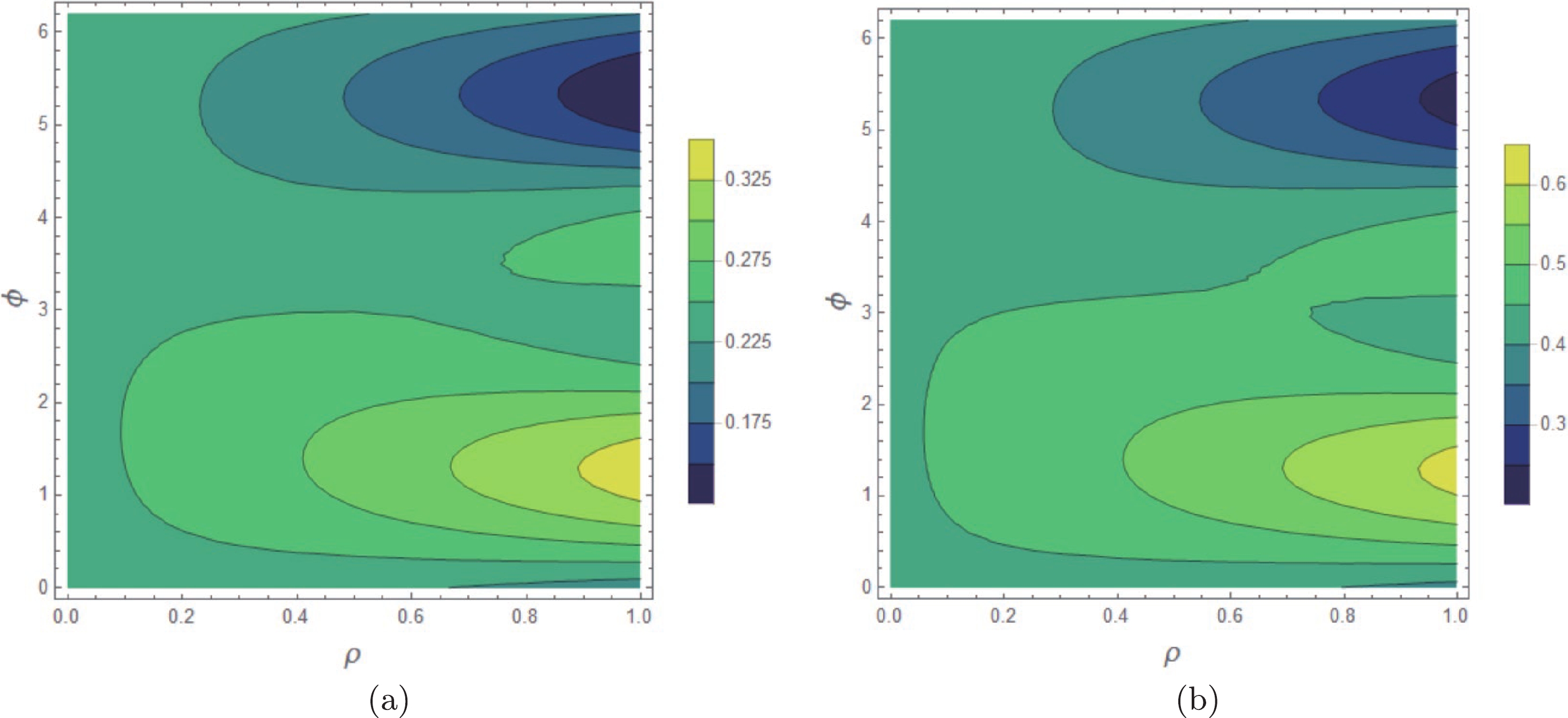
Figure 2. (color online) Localized
$ CP $ violation of the$ B^-\rightarrow K^-f_0 \rightarrow K^-\pi^+\pi^- $ decay (a) without the$ a_0^0(980)-f_0(980) $ mixing mechanism, (b) with the$ a_0^0(980)-f_0(980) $ mixing mechanism.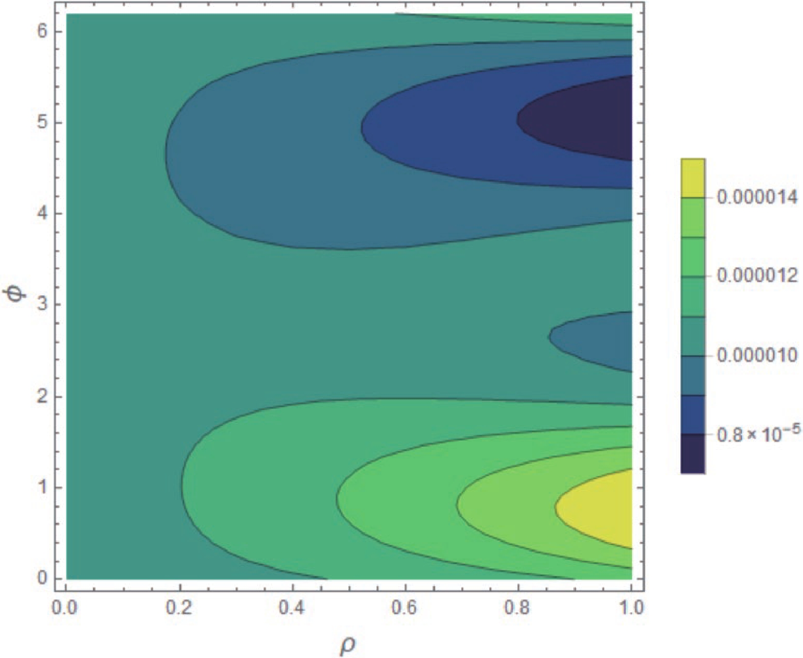
Figure 3. (color online) Branching fraction of the
$ B^-\rightarrow $ $ K^-f_0 \rightarrow K^-\pi^+\pi^- $ decay.In addition to the above specific calculations, from a logical perspective, we can perform the following analysis as in Ref. [45]. The width or the branching fraction of the cascade decay
$ B^-\rightarrow K f_0 \rightarrow K^-\pi^+\pi^- $ can be split into the weak decay$ B^-\rightarrow K f_0 $ and strong decay$ f_0\rightarrow \pi^+\pi^- $ , and can be replaced by the width relationship as$ \Gamma_{B^-\rightarrow K f_0 \rightarrow K^-\pi^+\pi^-}\propto \Gamma _{B^-\rightarrow K f_0} $ $ \Gamma_{f_0\rightarrow \pi^+\pi^-} $ adopting the narrow width approximation, with$ \Gamma_{B^-\rightarrow K f_0}\propto\mid M_{B^-\rightarrow K f_0}+ \Delta_{a_0f_0}M_{B^-\rightarrow K a_0}\mid^2 $ . The mixing term contribution is small, at most a few percent or less; hence, it is negligible to branching fraction. However, the mixing corrections behave differently for$ CP $ conjugate processes, which has been discussed in detail in Ref. [45];$ {\cal{A}}_{CP}(B^-\rightarrow K^- f_0(a_0) \rightarrow K^-\pi^+\pi^-)={\cal{A}}_{CP}^0+\Delta {\cal{A}}_{CP} $ with a Taylor expansion of$ {\cal{A}}_{CP} $ up to$ {\cal{O}}({\rm{mixing-term}}) $ , where$ {\cal{A}}_{CP}^0 $ and$ \Delta {\cal{A}}_{CP} $ are the$ CP $ violations without and only considering the$ a_0^0(980)- f_0(980) $ mixing effect, respectively. From our calculation, we can derive$ \Delta {\cal{A}}_{CP}=0.191\pm0.087 $ which is comparable to the value of$ {\cal{A}}_{CP}^0=0.232\pm0.106 $ and cannot be ignored. These analysis are consistent with the above calculations. Therefore, we propose that the$ a_0^0(980)-f_0(980) $ mixing mechanism be extended and applied to other decays. -
In this paper, we have studied the localized integrated
$ CP $ violation of the$ B^-\rightarrow K^-f_0(a_0) \rightarrow K^-\pi^+\pi^- $ decay considering the$ a_0^0(980)-f_0(980) $ mixing mechanism in the QCD factorization approach. We observe that the localized integrated$ CP $ violation is enlarged owing to the$ a_0^0(980)- f_0(980) $ mixing effect. Without the$ a_0^0(980)- f_0(980) $ mixing, the localized$ CP $ violation is observed to be$ {\cal{A}}_{CP}(B^-\rightarrow K f_0 \rightarrow K^-\pi^+\pi^-)=[0.126, 0.338] $ ($ 0.232\pm 0.106 $ with the central value form), while$ {\cal{A}}_{CP}(B^-\rightarrow K^- f_0(a_0) \rightarrow K^-\pi^+\pi^-)=[0.230, 0.615] $ ($ 0.423\pm0.193 $ with the central value form) when this mixing effect is considered. Meanwhile, the$ CP $ violation caused by the mixing term$ \Delta{\cal{A}}_{CP}=0.191\pm0.087 $ is comparable to that of$ {\cal{A}}_{CP}^0= 0.232\pm0.106 $ when the mixing effect is not considered; therefore, we cannot easily ignore the contribution from the$ a_0^0(980)-f_0(980) $ mixing effect. In addition, we also calculate the branching fraction of the$ B^-\rightarrow K^-f_0 \rightarrow K^-\pi^+\pi^- $ decay and obtain$ {\cal{B}}(B^-\rightarrow K f_0 \rightarrow K^-\pi^+\pi^-)= [7.150, 14.89]\times10^{-6} $ as shown in Fig. 3, which agrees well with the experimental result$ {\cal{B}}(B^-\rightarrow K f_0 \rightarrow K^-\pi^+\pi^-)= 9.4^{+1.0}_{-1.2}\times 10^{-6} $ . The mixing corrections for the branching fraction behave differently for$ CP $ conjugate processes, as mentioned in Sect. IV. Since the mixing term is very small, often a few percent or even less, while calculating the branching fraction, we can ontain the approximation$ {\cal{B}}(B^-\rightarrow K^- f_0(a_0)\rightarrow K^-\pi^+\pi^-)\approx {\cal{B}}(B^-\rightarrow K f_0 \rightarrow K^-\pi^+\pi^-) $ by ignoring the$ a_0^0(980)-f_0(980) $ mixing effect. However, for$ CP $ violation, this mixing effect contributes significantly and cannot be neglected. The same scenario is also expended for other B or D mesons decay channels. Thus, we suggest that$ a_0^0(980)-f_0(980) $ mixing mechanism should be considered when studying the heavy meson decays both theoretically and experimentally when this mixing effect can exist. -
One of the authors (J.-J. Qi) thanks Professor Zhi-Qing Zhang for helpful discussions.
-
In the numerical calculations, we should input distribution amplitudes and the CKM matrix elements in the Wolfenstein parametrization. For the CKM matrix elements, which are determined from experiments, we use the results in Ref. [43]:
$ \begin{aligned}[b]&\bar{\rho}=0.117\pm0.021, \quad \bar{\eta}=0.353\pm0.013, \\& \lambda=0.225\pm0.00061,\quad A=0.811^{+0.023}_{-0.024},\end{aligned}\tag{A1}$

where
$ \bar{\rho}=\rho\left(1-\frac{\lambda^2}{2}\right), \quad \bar{\eta}=\eta\left(1-\frac{\lambda^2}{2}\right).\tag{A2} $

The Wilson coefficients used in our calculations are obtained from Refs. [46–49]. It should be noted that the convention in this work is different from that in Ref. [46] for the effective Hamiltonian (from the expressions of the
$ Q_{1, 2}^p $ ), so we adopt$ c_1=1.1502 $ and$ c_2=-0.3125 $ :$\begin{aligned}[b] &c_1=1.1502, \quad c_2=-0.3125,\quad c_3=0.0174,\\& c_4=-0.0373,\quad c_5=0.0104,\quad c_6=-0.0459,\\&c_7=-1.050\times10^{-5},\quad c_8=3.839\times10^{-4}, \\& c_9=-0.0101,\quad c_{10}=1.959\times10^{-3}. \end{aligned}\tag{A3}$

For the masses of mesons appeared in B decays, we use the following values [43] (in units of GeV):
$ \begin{aligned}[b]&m_{B^-}=5.279,\quad m_{K^-}=0.494,\quad m_{f_0(980)}=0.990,\\& m_{a_0^0(980)}=0.980,\quad m_{\pi^\pm}=0.14, \end{aligned}\tag{A4}$

whereas, for the widths we use (in
$ {\rm{GeV}} $ ) [43]$ \Gamma_{f_0(980)}=0.074,\quad\Gamma_{a_0^0(980)}=0.092. \tag{A5}$

The pole masses of quarks are [43] (in
$ {\rm{GeV}} $ ):$ \begin{aligned}[b]&m_u=m_d=0.0035, \quad m_b=4.78,\\& m_q=\frac{m_u+m_d}{2},\quad m_c=1.67. \end{aligned}\tag{A6}$

The running masses of quarks are [5, 43] (in
$ {\rm{GeV}} $ ):$ \begin{aligned}[b]&m_s(1{\rm{GeV}})=0.119,\quad m_c(m_c)=1.30, \\& m_b(m_b)=4.20, \quad \frac{m_s(\mu)}{m_{u,d}(\mu)}=27.5. \end{aligned}\tag{A7}$

The following numerical values for the decay constants are used [5, 50–52](in
$ {\rm{GeV}} $ ):$ \begin{aligned}[b]& f_{\pi^\pm}=0.131,\quad f_{B^-}=0.21\pm0.02, \\& f_{K^-}=0.156\pm0.007,\\& \bar{f}_{f_0(980)}=0.370\pm0.02, \\&\bar{f}_{a_0^0(980)}=0.365\pm0.02. \end{aligned}\tag{A8} $

For the form factors, we use [5]
$ \begin{aligned}[b]&F_0^{B\rightarrow K}(0)=0.35\pm0.04,\\& F_0^{B\rightarrow f_0(980)}(0)=0.25, \\& F_0^{B\rightarrow a_0^0(980)}(0)=0.25.\end{aligned}\tag{A9} $

The values of Gegenbauer moments at
$ \mu=1 {\rm{GeV}} $ are obtained from [5]:$ \begin{aligned}[b]& B_{1,f_0(980)}=-0.78\pm0.08,\quad B_{3,f_0(980)}=0.02\pm0.07,\\& B_{1,a_0^0(980)}=-0.93\pm0.10,\quad B_{3,a_0^0(980)}=0.14\pm0.08. \end{aligned} \tag{A10}$

Impact of ${ {\boldsymbol a}_{\bf 0}^{\bf {0}}(980)-{\boldsymbol f}_{\bf {0}}(980) }$ mixing on the localized CP violations of the ${{\boldsymbol B}^-{\bf\rightarrow} {\boldsymbol K}^- \boldsymbol\pi^+\boldsymbol\pi^- }$ decay
- Received Date: 2022-02-28
- Available Online: 2022-08-15
Abstract: In the framework of the QCD factorization approach, we study the localized


 DownLoad: