


 Abstract
 HTML
HTML Reference
 Related
 PDF
PDF


-
The anti-de Sitter/conformal field theory (AdS/CFT) correspondence has established a bridge between the boundary CFT and gravity in the bulk asymptotically AdS spacetime [1−3]. The correspondence also indicates an emergent picture of gravity, namely, the geometry and gravitational dynamics of bulk spacetime should in principle be constructed from the information of the boundary CFT, which is called the bulk reconstruction [4−10]. In the reconstruction of bulk gravitational theory, the notion of holographic entanglement entropy plays a key role [11−13], which states that the entanglement entropy of a boundary subregion A is a quarter of the area of a co-dimensional-2 minimal surface
$ {{\gamma _A}} $ growing into the bulk from the boundary of A (to leading order in the gravitational coupling constant G), i.e.,$ {S_A} = \frac{{\rm Area}(\gamma _A)}{4 G}. $

(1) Studies have shown that field theory information contained in the subregion A can determine the information in the spatial region bounded by A and the bulk extremal surface, which is called the entanglement wedge [4, 14, 15]. Subsequently, significant progress has been made along this direction, such as the reconstruction of bulk operators from the boundary CFT operators in subregions [4−10], generation of the bulk AdS geometry from the entanglement renormalization of the tensor networks [16−21], and investigation of the emergence of gravitational dynamics from the geometry generated from the tensor networks [22]. According to the RT formula (1), a boundary subregion A can at least detect the nonlocal information about the global configuration of the extremal surface
$ {{\gamma _A}} $ by reading out its classical area. However, how the information in A detects (or reconstructs) the information in the region inside the RT surface$ {{\gamma _A}} $ (i.e., the entanglement wedge of A) is not apparent and direct.In a recent paper, three of the present authors (Lin, Sun, and Sun) proposed a concrete and very natural approach to reconstructing the bulk geometry in the entanglement wedge from a surface growth procedure, similar to the Hygens' principle of wave propagation. The basic concepts of the approach can be briefly described as follows [23]. First, many minimal surfaces are "growing" out from a set of small boundary subregions side by side. Second, these minimal surface are considered to be the new boundaries, and the points on them are further considered to be the anchor points for the new minimal surfaces to grow into the deeper bulk regions. Subsequently, the procedure is repeated layer by layer such that the new minimal surfaces can probe arbitrary regions in the entanglement wedge. Consequently, the information of these bulk regions can be detected and reconstructed from the initial boundary regions in this manner (Fig. 1). A closely related case is the horizon entropy of the brane world black hole, in which its horizon extends into the bulk spacetime and it is exactly a minimal surface when the black hole is stationary, and then the black hole Bekenstein-Hawking entropy can be naturally interpreted as the holographic entanglement entropy between regions in and outside the black hole horzion [24]. The above picture can be explicitly realized by generalizing the one-shot entanglement distillation (OSED) method and the surface/state correspondence [25, 18], and the well-known MERA-like tensor network in [19−21] can be exactly identified with specific surface growth configurations [23], thus providing a concrete and intuitive method for the entanglement wedge reconstruction [4, 14, 15].
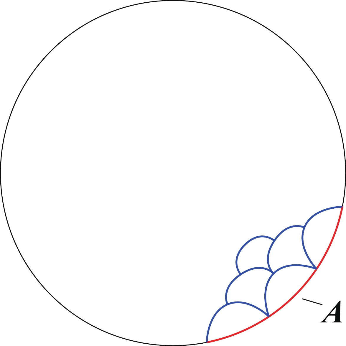
Figure 1. (color online) Illustration of the surface growth scheme with three layers.
Since the surface growth picture is a general geometric description that is independent of the tensor network, in this paper, we further analyze the surface growth approach in asymptotically AdS
$ _3 $ spacetime by directly calculating the minimal surfaces. We study both homogeneous and inhomogeneous subsystem cases and demonstrate that the spatial region inside the entanglement wedge can be efficiently reconstructed, similar to bubble growing, which presents a clear process of boundary to bulk propagation. -
In this section, we briefly review our previous study [23], which provided an interesting perspective on the surface growth scheme based on the tensor network (more explicitly, the so-called OSED tensor network).
The tensor network was originally used as a numerical simulation tool to effectively represent quantum many-body states in condensed matter physics. It is characterized by relating a bulk graph of a geometric structure with an entanglement structure of a quantum system. Later, specific types of tensor network models were tentatively used to describe the mechanism of the holographic duality [16−18, 26−29, 23].
The OSED tensor network is a tensor network model constructed based on the OSED procedure proposed in [18]. Let us first briefly describe the concept of OSED. Studies have shown that because of the holographic limits, we can always construct the so-called "smoothed states"
$ \left| {{\Psi ^\varepsilon }} \right\rangle $ and$ \rho _A^\varepsilon $ to approximate the given holographic CFT full, pure state$ \left| \Psi \right\rangle $ and the reduced density matrix$ {\rho _A} $ for a certain subregion A of the CFT. Subsequently, by rearranging the eigenvalues of the smoothed state$ \rho _A^\varepsilon $ in descending order and dividing them into blocks of size$ \Delta = {{\rm e}^{{S_A} - O(\sqrt {{S_A}})}} $ , we can further approximate the boundary state$ \left| \Psi \right\rangle $ as the following tensor network representation (see more details in [18, 23]):$ {\Psi ^{A \bar A}} = {W_1}_{\bar{\beta} \bar{\alpha}}^{A}{W_2}_{\beta \alpha }^{\bar A}\phi ^{\alpha \bar \alpha}{\sigma ^{\beta \bar \beta}} = ({W_1} \otimes {W_2})(\left| \phi \right\rangle \otimes \left| \sigma \right\rangle), $

(2) where a maximally entangled state
$ \left| \phi \right\rangle \otimes \left| \sigma \right\rangle $ has been distilled out, which is defined by$ \begin{aligned}[b] & \left| \phi \right\rangle = \sum\limits_{m = 0}^{{{\rm e}^{S - O(\sqrt S )}}} {{{\left| {m\bar m} \right\rangle }_{\alpha \bar \alpha }}}, \\& \left| \sigma \right\rangle = \sum\limits_{n = 0}^{{{\rm e}^{O(\sqrt S )}}} {\sqrt {\tilde p _{n\Delta }^{{\rm avg}}} {{\left| {n\bar n} \right\rangle }_{\beta \bar \beta}}}, \end{aligned} $

(3) where S is the entanglement entropy of A, and
$ {{\tilde p _{n\Delta }}^{\rm avg}} $ is the average eigenvalue of each block. Clearly, the logarithm of the Hilbert space dimension of$ \left| \phi \right\rangle $ matches the entanglement entropy of A, and$ \left| \sigma \right\rangle $ acts as the quantum fluctuation. The tensors$ {W_1} $ and$ {W_2} $ are isometries, which map the auxiliary states represented by the bonds of$ {\phi ^{\alpha\bar \alpha}}{\sigma ^{\beta \bar \beta}} $ into the eigenstates of the reduced density matrices for A and$ \bar A $ , respectively. Eq. (2) is the OSED for a holographic state (Fig. 2(a)).
Figure 2. (color online) (a) Simplest OSED tensor network for a bipartite holographic state. (b) Another example: a special OSED tensor network with spherical symmetry and fractal characteristics. It can be identified with the well-known MERA-like tensor network.
Subsequently, utilizing a series of nonintersecting RT surfaces starting from the boundary to discretize the bulk spacetime into cells according to appropriate order①, Ref. [18] showed that by iterating the OSED procedure on a holographic boundary state, an isometry tensor can be assigned for each cell to implement the map between the states associated with its minimal surface boundaries, and finally, an entire OSED tensor network can be constructed, which can reproduce the correct boundary state with high fidelity and have a bulk geometry that perfectly matches the bulk AdS spacetime. Interestingly, in [23], we constructed a special OSED tensor network with spherical symmetry and fractal feature in this manner (Fig. 2(b)), and we demonstrated that it can be identified with the well-known MERA-like tensor network.
Moreover, in [23], we further investigated the physical meaning of the OSED tensor network. More specifically, a mixed state
$ \{ (\left| {\bar m} \right\rangle,{p_m} = {1}/{{{{\rm e}^S}}})\} $ with equal probabilities to each extremal surface in the bulk is assigned, since in the framework of surface/state correspondence the density matrix corresponding to an extremal surface is a direct product of density matrices at each point. Therefore, the isometry tensor in the OSED tensor network plays the role of implementing the entanglement distillation procedure on the state of the union of the minimal surfaces in the previous layer and then maps it into the state on the next minimal surfaces. This understanding results in the generalization of the OSED tensor network into cases involving more general bulk minimal surfaces whose anchor points are located on the previous bulk minimal surface. Therefore, the generalized OSED tensor network provides a natural interpretation for our surface growth scheme, namely, the emergence of bulk spacetime geometry can be interpreted as layers of minimal surfaces continue to grow into the deeper bulk regions from the initial boundary regions. -
Now, let us discuss the direct growth of bulk minimal surface in pure AdS
$ _3 $ spacetime in the global coordinate$ {\rm d}s^2={\rm d}\rho^2+L^2\left(-\cosh^2\frac{\rho}{L}{\rm d}t^2+\sinh^2\frac{\rho}{L}{\rm d}\phi^2\right), $

(4) where L is the curvature radius of the AdS spacetime. The bulk static co-dimensional-2 surface (which is a curve for AdS
$ _3 $ ) can be expressed as$ \rho=\rho(\phi) $ . Subsequently, the length of the curve is$ \gamma =\int\sqrt{\left(\rho'^2+L^2\sinh^2\frac{\rho}{L}\right)}{\rm d}\phi{}\equiv \int\mathcal{L}{\rm d}\phi, $

(5) where
$ \rho'={{\rm d}\rho}/{{\rm d}\phi} $ . The bulk minimal surface satisfies the Euler-Lagrange equation$ \frac{\partial \mathcal{L}}{\partial\rho}-\frac{\rm d}{{\rm d}\phi}\frac{\partial\mathcal{L}}{\partial\rho'}=0, $

(6) which gives
$ \tilde{\rho}''\sinh\tilde{\rho}-2\tilde{\rho}'^2\cosh\tilde{\rho} -\sinh^2\tilde{\rho} \cosh\tilde{\rho} =0, $

(7) where
$ \tilde{\rho}\equiv\rho/L $ . Eq. (7) can be solved as$ \begin{aligned}[b] \phi =&\pm\arctan\left(\frac{\sinh^2\tilde{\rho}}{\sinh\tilde{\rho}_*} +\cosh\tilde{\rho}\sqrt{\frac{\sinh^2\tilde{\rho}}{\sinh^2\tilde{\rho}_*}-1}\right){}\\ &\mp \arctan\left(\sinh\tilde{\rho}_*\right)+\phi_0, \end{aligned}$

(8) in which
$ \rho_* $ is the turning point of the bulk geodesic and$ \phi_0=\phi(\rho_*) $ . Note that the value of$ \rho_* $ will change for different bulk geodesics. Substituting Eq. (8) into Eq. (5), the length of the geodesic becomes$ \gamma=L\ln\frac{\left(\cosh\tilde{\rho}_1+\sqrt{\sinh^2\tilde{\rho}_1-\sinh^2\tilde{\rho}_*} \right)\left(\cosh\tilde{\rho}_2+\sqrt{\sinh^2\tilde{\rho}_2-\sinh^2\tilde{\rho}_*} \right)}{\cosh^2\tilde{\rho}_*}, $

(9) where we require that
$ \tilde{\rho}_*<\tilde{\rho}_1<\tilde{\rho}_2 $ .Note that for a given angular size
$ 2(\phi-\phi_0) $ of the subsystem A, Eq. (8) fixes the bulk geodesic grown from A by relating the initial radial (cutoff) position$ \tilde{\rho}=\tilde{\rho}_c $ of A to the turning point position$ \tilde{\rho}_* $ . We can then draw the bulk growing minimal curves by iterating this process during which different$ \tilde{\rho}_* $ positions are obtained from different starting positions$ \tilde{\rho}_c $ of the previous step. Now, we can draw the surface growth picture as shown in Fig. 3. At the conformal boundary, we first select ten subsystems with equal spatial size, each of which expands at an angle$ \phi=\pi/25 $ . After the growth of the first layers of the geodesics, we select the boundaries of the second layers of geodesics to be at the centers of the first ones; then, the bulk space within the entanglement wedge can be filled after finite steps. An interesting point is that, the outer bulk geodesic that corresponds to all ten subregions (i.e., subsystem A) also should be treated as the spatial boundary when considering the surface growth. Otherwise, the region growing from the ten subregions will be smaller than the outer entanglement wedge.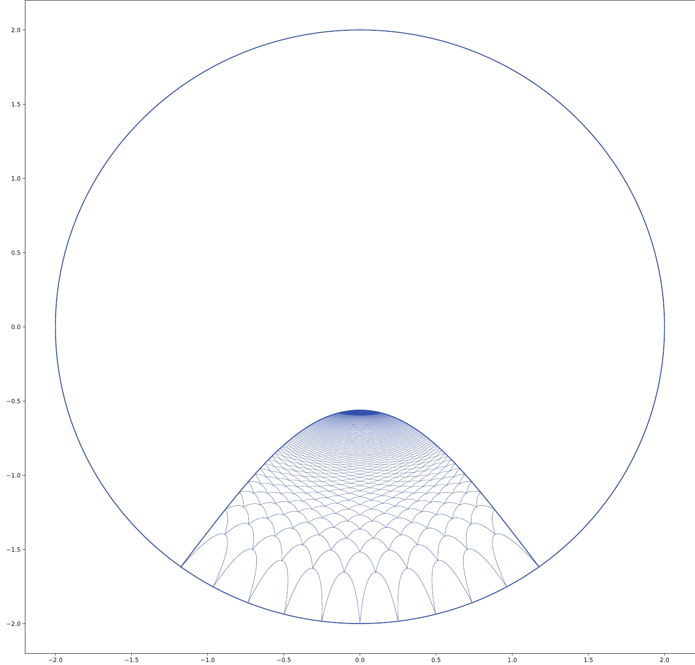
Figure 3. (color online) Surface growth for initial ten subsystems with equal spatial size, where each subsystem expands an angle
$ \phi=\pi/25 $ , the conformal boundary is selected as$ \rho_0=2 $ and$ L=0.5 $ , and the growing steps are 300.We can also consider the surface growth for ten subregions with arbitrary sizes on the boundary (Fig. 4). Because the subregions have different sizes, from the second layer on, some minimal surfaces become asymmetric; thus, when considering the new geodesics connecting two adjacent geodesics, we select the one with the maximal value. Similar to the symmetric case in Fig. 3, the outer boundary (the minimal surface corresponding all subregions) is necessary for the growing minimal surfaces to fill the entanglement wedge.

Figure 4. (color online) Surface growth for the initial ten subsystems with different spatial sizes, and the conformal boundary is selected as
$ \rho_0=2 $ and$ L=0.5 $ ; the growing steps are 300.Another interesting case is to construct the full AdS space from the surface growth. To achieve this, we can divide the entire boundary into many subregions. Without loss of generality, we select twenty subregions with identical sizes as in Fig. 5 and select the boundaries of the next layers of minimal surfaces to be the centers of the previous layers. After finite steps of minimal surface growing, the full AdS space is filled or constructed.
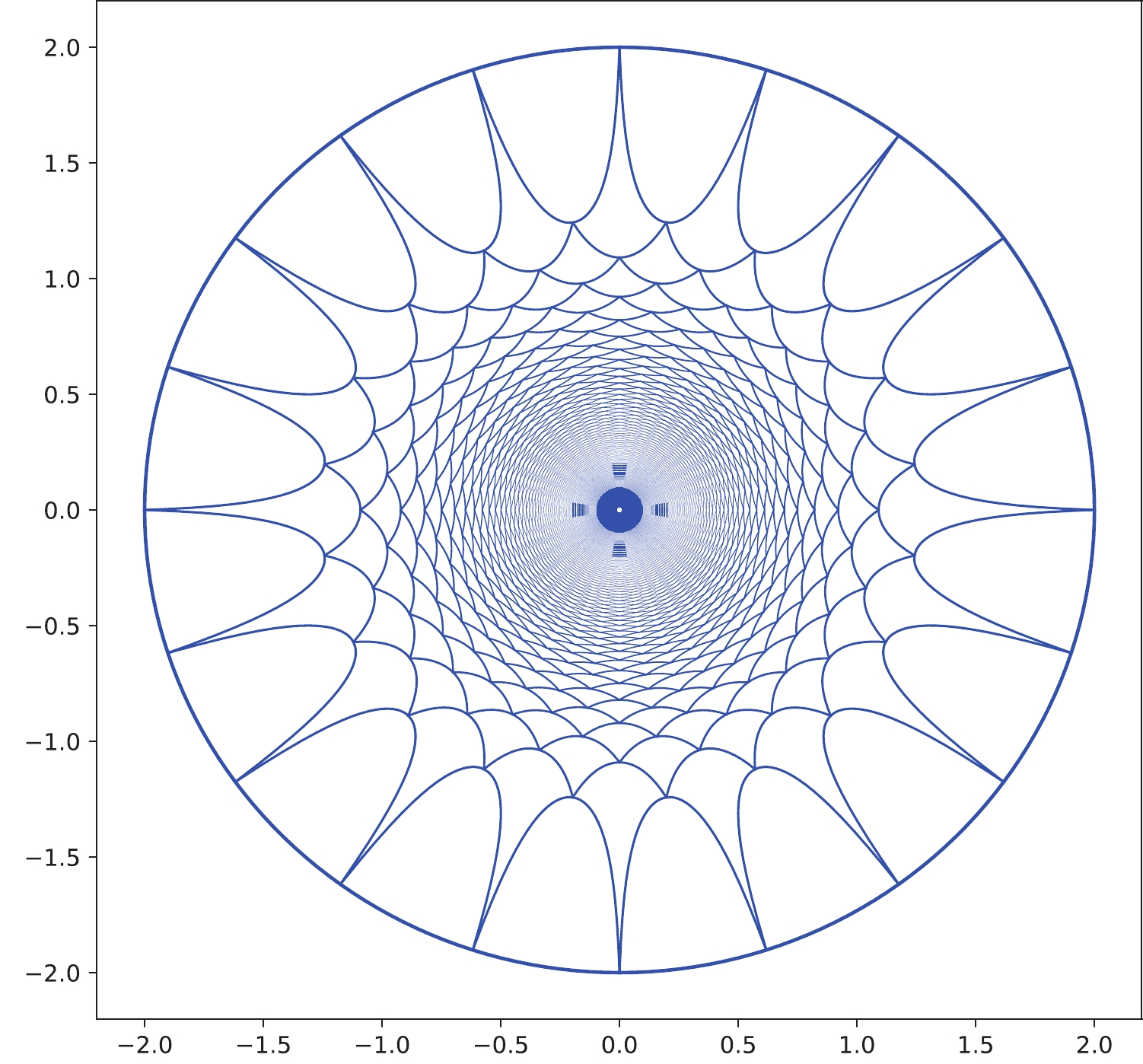
Figure 5. (color online) Surface growth from the entire boundary when they are divided into twenty subsystems with equal spatial size, where each subsystem expands at an angle
$ \phi=\pi/10 $ , and the conformal boundary is selected as$ \rho_0=2 $ and$ L=0.5 $ ; the growing steps are also 300. -
In this section, we study the bulk reconstruction from surface growth in a nonrotating BTZ black hole. The metric of the nonrotating BTZ black hole is [30, 31]
$ {\rm d}s^2=-\frac{r^2}{L^2}f(r){\rm d}t^2+\frac{L^2}{r^2 f(r)}{\rm d}r^2+r^2 {\rm d}\phi^2, $

(10) where
$ f(r)=1-\dfrac{M}{r^2} $ and its horizon is located at$ r_h=\sqrt{M} $ . The bulk static curve is$ r=r(\phi) $ , which has a length of$ \gamma=\int {\rm d}\phi\sqrt{g(r)\dot{r}^2+r^2}, $

(11) where
$ g(r)=\dfrac{L^2}{r^2 f(r)} $ and$ \dot{r}=\dfrac{{\rm d}r}{{\rm d}\phi} $ . The bulk geodesic is determined using the Euler-Lagrange equation, which yields$ 2r^2+4gu^2-rg'u^2-2gruu'=0, $

(12) with
$ u=u(\phi)\equiv \dot{r} $ and$ g'=\dfrac{{\rm d}g}{{\rm d}r} $ . Eq. (12) can be solved as$ u(\phi)\equiv \frac{{\rm d}r}{{\rm d}\phi}=\pm\sqrt{\frac{r^4-r^2r_*^2}{r_*^2g(r)}}, $

(13) where
$ r_* $ indicates the turning point of the bulk geodesic. Subsequently, we can obtain the solution$ \begin{aligned}[b] \pm(\phi-\phi_0)=&-\frac{L}{r_h}\ln\left(\sqrt{1-\frac{r_h^2}{r^2}}-\sqrt{\frac{r_h^2}{r_*^2}-\frac{r_h^2}{r^2}}\right)\\& +\frac{L}{r_h}\ln\sqrt{1-\frac{r_h^2}{r_*^2}}, \end{aligned} $

(14) where
$ \phi_0=\phi(r_*) $ denotes the center of the bulk geodesic. Consequently, the length for the bulk geodesic is$ \gamma=L\cosh^{-1}\left(\frac{2r_1^2-(r_h^2+r_*^2)}{r_*^2-r_h^2}\right)+L\cosh^{-1}\left(\frac{2r_2^2-(r_h^2+r_*^2)}{r_*^2-r_h^2}\right), $

(15) in which we require that
$ r_*<r_1<r_2 $ and$ \phi(r_1)<\phi_0<\phi(r_2) $ .Note that Eq. (14) determines the configurations of bulk geodesics in the BTZ black hole. Similar to the AdS case, for a given angular size
$ 2(\phi-\phi_0) $ of the subsystem A located at the radial cutoff position$ r=r_c $ , Eq. (14) fixes a corresponding turning point position$ r_* $ . Subsequently, the bulk growing minimal curves can be drawn by iterating this process during which different$ r_* $ positions are obtained from different starting positions$ r_c $ of the previous step. Let us consider the surface growth from ten boundary subregions with equal sizes, where each subregion expands at an angle of$ \pi/25 $ , and also select the boundaries of the next layers of minimal surfaces to be the centers of the previous layers. As shown in Fig. 6, owing to the existence of black hole horizon, the growing minimal curves (together with the outer bulk minimal curve of the subsystem A) can surround the horizon after finite growing steps [32]②.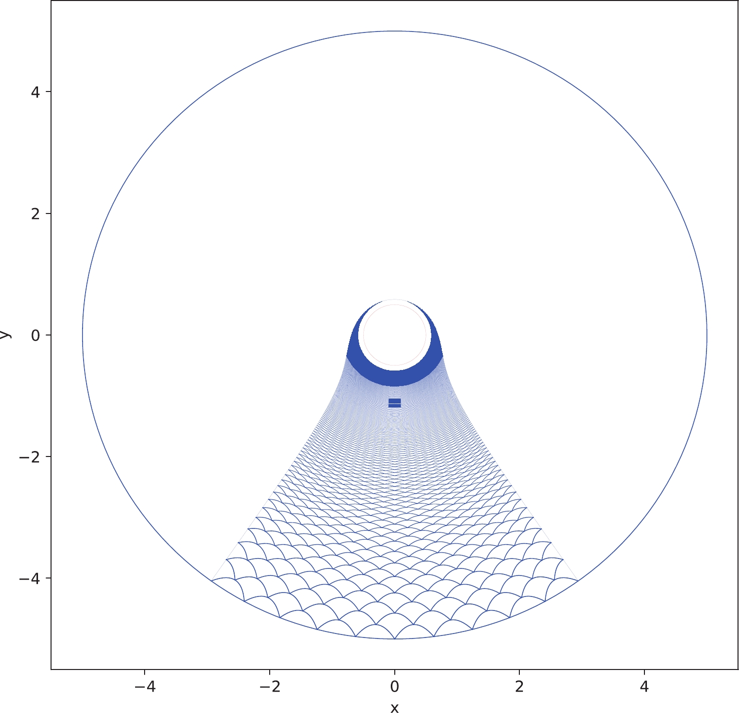
Figure 6. (color online) Surface growth from ten boundary subregions with equal size, where each subsystem expands at an angle
$ \phi=\pi/25 $ , and the conformal boundary is selected as$ r_0=5 $ , the AdS curvature radius is$ L=1 $ , and the black hole horizon radius is$ r_h=0.5 $ ; the growing steps are 360.Note that the asymptotic boundary of the AdS spacetime is located at
$ r\rightarrow \infty $ . However, this will not affect the bulk reconstruction from the surface growth. Because the surface growth process corresponds to the holographic renormalization group flow, or the MERA of the corresponding tensor network [23], the bulk minimal surfaces can grow from any finite cutoff surfaces$ r=r_c $ . For example, we can select the cutoff surface to be located at$ r_0=r_c=20 $ and also consider ten homogeneous subregions (Fig. 7). By comparing Fig. 7 with Fig. 6, we observe that after very few steps of surface growing, the minimal surfaces in Fig. 7 will reach the region$ r_c=5 $ .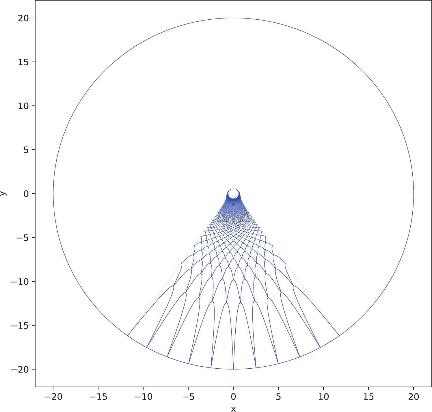
Figure 7. (color online) Surface growth from ten boundary subregions with equal size, where each subsystem expands at an angle
$ \phi=\pi/25 $ , the cutoff surface is selected as$ r_0=r_c=20 $ , the AdS curvature radius is$ L=1 $ , and the black hole horizon radius is$ r_h=0.5 $ ; the growing steps are also 360.As a final example, we consider the surface growth from ten inhomogeneous subsystems at a cutoff surface
$ r_c=5 $ (Fig. 8). Again, from the second layer on, the boundary points of some of the geodesics cannot end at the center of the previous layers; instead, we must select the maximal one connecting the adjacent two geodesics in the previous layer. In addition, Fig. 8 shows that as the geodesics grow deeper into the BTZ black hole, the surface growth configuration becomes more homogeneous.
Figure 8. (color online) Surface growth from ten inhomogeneous boundary subsystems, where all subsystems expand at an angle
$ \phi=2\pi/5 $ , and the cutoff surface is selected as$ r_0=r_c=5 $ . Additionally, the AdS curvature radius is$ L=1 $ , the black hole horizon radius is$ r_h=0.5 $ , and the growing steps are 358. -
In this study, we further investigate the surface growth approach for bulk reconstruction by directly analyzing the growth of bulk minimal surfaces (geodesics) in asymptotically AdS
$ _3 $ spacetime③. We show using various cases that the spatial region in the outer entanglement wedge can be constructed from the growth of the bulk minimal surfaces layer by layer, which provides further support for the surface growth approach and presents a clear picture of the boundary to bulk propagation and subregion to subregion duality in the gauge/gravity duality. In addition, in the surface growth scheme, each previous layer of growing minimal surfaces acts as the new boundary for the next layer. This corresponds to the holographic Wilsonian renormalization group flow, in which the effective field theory can be located at any radial cutoff surface from UV to IR regions [33, 34]. Moreover, the surface growth process corresponds to the extended OSED tensor network, and it is also shown to be closely related to the entanglement of purification and bit threads description for bulk reconstruction [35, 36]. The surface growth approach provides a concrete and intuitive realization of the subregion duality and an efficient method for reconstructing bulk geometry and matter fields. Many interesting problems can be explored with the surface growth approach such as studying its relation with the$ T\bar{T} $ deformation in the dual CFT [37, 38] and the perturbative corrections during the surface growth [39]. -
We would like to thank L.-Y. Hung for helpful discussions.
Note on surface growth approach for bulk reconstruction
- Received Date: 2022-02-22
- Available Online: 2022-08-15
Abstract: In this paper, we show using several examples that the bulk geometry of asymptotically AdS


 DownLoad: